46 Acd 2009
•
0 gostou•437 visualizações

7th Workshop on Advanced Control and Diagnosis The Workshop on Advanced Control and Diagnosis (ACD) organised by the European Institute for Applied Research (IAR) brought together academics and engineers in control engineering and computer science.

Recomendados
Recomendados
Mais conteúdo relacionado
Semelhante a 46 Acd 2009
Semelhante a 46 Acd 2009 (20)
Último
Último (20)
46 Acd 2009
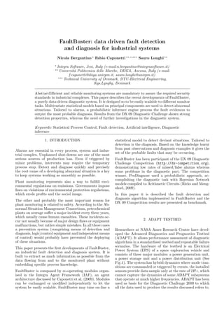
- 1. FaultBuster: data driven fault detection and diagnosis for industrial systems Nicola Bergantino ∗ Fabio Caponetti ∗∗,∗,∗∗∗ Sauro Longhi ∗∗ ∗ Integra Software, Jesi, Italy (e-mail:n.bergantino@integrasoftware.it) ∗∗ Universit` Politecnica delle Marche, DIIGA, Ancona, Italy (e-mail: a f.caponetti@diiga.univpm.it, sauro.longhi@univpm.it) ∗∗∗ Technical University of Denmark, DTU-Electrical Engineering, Kgs.Lyngby, Denmark AbstractEfficient and reliable monitoring systems are mandatory to assure the required security standards in industrial complexes. This paper describes the recent developments of FaultBuster, a purely data-driven diagnostic system. It is designed so to be easily scalable to different monitor tasks. Multivariate statistical models based on principal components are used to detect abnormal situations. Tailored to alarms, a probabilistic inference engine process the fault evidences to output the most probable diagnosis. Results from the DX 09 Diagnostic Challenge shown strong detection properties, whereas the need of further investigations in the diagnostic system. Keywords: Statistical Process Control, Fault detection, Artificial intelligence, Diagnostic inference 1. INTRODUCTION statistical model to detect deviant situations. Tailored to detection is the diagnosis. Based on the knowledge learnt from past observations and diagnosis examples it gives the Alarms are essential in every process, system and indus- set of the probable faults that may be occurring. trial complex. Unplanned shut-downs are one of the most serious sources of production loss. Even if triggered by FaultBuster has been participant of the DX 09 Diagnostic minor problems, intervents may require the temporary Challenge Competition (http://dx-competition.org), process stop. Detect and diagnose quickly and precisely demonstrating low rates of missed/false alarms whereas the root cause of a developing abnormal situation is a key some problems in the diagnostic part. The competition to keep systems working as smoothly as possible. winner, ProDiagnose used a probabilistic approach, ac- complishing the diagnostic task with Bayesian Network Plant monitoring represents also a way to fullfill envi- models compiled to Arithmetic Circuits (Ricks and Meng- ronmental regulations on emissions. Governments impose shoel, 2009). fines on violations of environmental protection regulations, which erode profits and the social image. In this paper it is described the fault detection and diagnosis algorithm implemented in FaultBuster and the The other and probably the most important reason for DX 09 Competition results are presented as benchmark. plant monitoring is related to safety. According to the Ab- normal Situation Management Consortium, petrochemical plants on average suffer a major incident every three years, which usually cause human casualties. These incidents oc- cur not usually because of major design flaws or equipment 2. ADAPT TESTBED malfunctions, but rather simple mistakes. In all these cases a prevention system (comprising means of detection and Researchers at NASA Ames Research Centre have devel- diagnosis, logic/control equipment and independent means oped the Advanced Diagnostics and Prognostics Testbed of control) would probably have prevented the deploying (ADAPT). It allows performance assessment of diagnostic of these situations. algorithms in a standardised testbed and repeatable failure This paper presents the first developments of FaultBuster, scenarios. The hardware of the testbed is an Electrical an industrial fault detection and diagnosis system. It is Power System (EPS) of a space exploration vehicle and built to extract as much information as possible from the consists of three major modules: a power generation unit, data flowing from and to the monitored plant without a power storage unit and a power distribution unit (See embedding specific process knowledge. Fig.1). The system has hybrid dynamics where mode tran- sitions are commanded or triggered by events. the installed FaultBuster is composed by co-operating modules organ- sensors provide data sample only at the rate of 2Hz, which ised in the Integra Agent Framework (IAF), an agent cannot capture the dynamics of some ADAPT subsystems architecture discussed by Caponetti et al. (2009). Modules that operate at much higher frequencies. ADAPT has been can be exchanged or modified independently to let the used as basis for the Diagnostic Challenge 2009 to which system be easily scalable. FaultBuster may tune on-line a all the data used to produce the results discussed refers to.
- 2. Load Bank 1 LT 500 Battery Cabinet TE TE 500 133 LGT400 ESH 170 TE LGT401 501 TE LGT402 L1A 128 TE EY170 502 ISH ESH ESH ISH ISH ESH E135 E140 E161 E165 E167 136 141A 160A 162 166 171 INV ST BAT1 FAN415 515 L1B CB136 IT140 EY141 EY160 IT161 CB162 1 ST CB166 IT167 XT167 EY171 ESH 165 ESH 172 TE 129 144A FAN480 L1C 120V AC >> EY172 ESH EY144 173 LGT481 L1D EY173 ESH E142 174 FT PMP425 525 L1E EY174 ESH 175 TE LGT411 511 L1F EY175 TE ISH ESH E181 228 180 183 ISH ESH DC482 E235 236 E240 241A L1G CB180 EY183 BAT2 CB236 E242 IT181 ESH 184 IT240 EY241 ESH 24V DC >> L1H TE 229 244A EY184 EY244 Load Bank 2 ESH ADAPT-Lite 270 FT PMP420 520 L2A EY270 ESH ISH ISH ESH E261 E265 E267 260A 262 266 271 INV LGT410 TE 510 L2B EY260 IT261 CB262 2 ST CB266 IT267 XT267 EY271 ESH 265 272 TE FAN483 L2C 328 120V AC >> ISH ESH EY272 E335 E340 ESH 336 341A 273 LGT484 L2D BAT3 CB336 LT IT340 EY341 EY273 505 ESH 274 TE TE ESH 505 329 344A LGT405 L2E TE EY274 LGT406 506 ESH EY344 275 LGT407 TE 507 Sensor Symbols ISH EY275 ESH E281 ST Circuit Breaker 280 283 FAN416 516 L2F E Voltage ISH ST Speed Position Feedback Relay Position CB280 EY283 L2G ESH IT Current TE Temperature ESH Feedback IT281 284 FT Flow LT Light XT Phase Angle 24V DC >> DC485 L2H EY284 Figure 1. The ADAPT Tier 2 EPS. ADAPT Tier 1 (Lite) is a subset of Tier 2. (Courtesy of Tolga Kurtoglu) 3. FAULTBUSTER statistics of the data projected through the model. Once an alarm is issued the contribution of each sensor to the FaultBuster is engineered to fullfill the requirements of abnormal situation is determined. In this way, the vector a fast, accurate, reliable and reconfigurable diagnostic of contribution rates represents the fault pattern that an system. Opposite and tight constraints lead to implement inference engine based on Markov logic networks has to a tradeoff solution. interpret. The inference output is the set of most probable faults. Fig. 2 shows the concept scheme of the system. The system was born to supervise tightly coupled, complex industrial systems. Quite often poor process knowledge is 3.1 Statistical model available, whereas huge archives of data may be accessible. This is the case when small-medium enterprises wants FaultBuster can be bootstrapped on a pre built model to improve their throughput and quality by monitoring or configured to fit on-line a PCA model. For industrial already running machinery. systems, with slow dynamics, a pre-built model adapted on-line would be the best option. Due to the high number Statistical process monitoring techniques have been heav- of working modes which ADAPT may present and the ily researched in the last few years. Multivariate statistical limited amount of available training examples available, methods based on Principal Component Analysis (PCA), a pre-built model resulted to be too conservative. partial Least Squares, and Independent Component Anal- ysis have been used and extended with success in various ADAPT works fault-less for 30s after a boot. The first applications (Qin, 2009; Liu et al., 2009; Du et al., 2007; observations collected on-line compose a training dataset Al Ghazzawi and Lennox, 2008; Liu et al., 2005; Bakshi, constructed in a way that columns represent the monitored 1998). variables (m) and each row an observation (n). FaultBuster processes all the observations using a statis- X ∈ A(n×m) tical reference model and an adaptive detection scheme. Because of the different magnitude of variables, the dataset Detection is based on residuals built from multivariate is standardised to null mean and unit variance. Boolean
- 3. PCA Least Model Squares ^ ^ ^ X S R MEWMA Kalman Filter X PCA Detection Projection ~ ~ Logic Alarms X ~ S R MEWMA Kalman Filter Least Back Squares Propagation Fault signature Markov Logic Networks Diagnosis Figure 2. Concept scheme of FaultBuster. observations from ADAPT are fed to the model by adding Two statistical distance measures are commonly computed a Gaussian noise with small standard deviation to the true to generate residual signals, the Hotelling’s T 2 and the value. squared prediction error (SP E) −1/2 The dataset can be decomposed as: T 2 (x) =||Dλk P T x||2 , (4) ˆ X = X + E, (1) 2 SP E(x) =||˜|| = x (I − P P )x. x T T (5) The matrices X ˆ and E represent the modeled and the Where −1/2 Dλk = −1/2 diag(λi ) with λi=1,...,l equal to the residual variation of X. first l eigenvalues of the correlation matrix R. ˆ X =T P T , Both statistics can be evaluated against fixed thresholds ˆˆ E =T P T , designed on the average run length (ARL). Due to the where T ∈ n×d and P ∈ m×1 are the score and loading hybrid nature of ADAPT, poor results have been obtained matrices. utilising fixed thresholds. As done previously by Wang and Tsung (2008), FaultBuster tries to improve the detection The decomposition of X is such that the matrix [P P T ] performances by using a predictor on the PCA subspaces is orthonormal and [T T T ] is orthogonal. The columns of issuing an alarm only after violation of an adaptive thresh- P are eigenvectors of the correlation matrix R associated old. ˆ to the largest l eigenvalues. The columns of P are the A multivariate exponentially weighted moving average remaining eigenvectors of R. The correlation matrix is (MEWMA) is used in each subspace (xp may be x or x) to ˆ ˜ evaluated on the scaled dataset as overcome the T 2 chart limitations (Montgomery, 2005). 1 R= XX T Zi = αxp + (1 − α)Zi−1 , (6) n−1 i The PCA model partitions the measurement space (m where 0 < α ≤ 1 and Z0 = 0. The control chart is dimensional) into two orthogonal subspaces. One spanned T 2 (Zi ) = Zi Σ−1 Zi , T Zi (7) by the first l principal components, in which the normal where the covariance matrix is data variations should occur, and a residual space where α abnormal situations and noise fall. The interested reader ΣZi = 1 − (1 − α)2i Σ, (8) 2−α may refer to Jackson (1991). where Σ is a diagonal matrix containing the eigenvalues of Once a command is issued, ADAPT is supposed to change R corresponding to the subspace considered. working mode. Several solution may be appliable to con- The MEWMA signals are monitored by a set of Kalman tinue the monitoring, e.g. a new PCA model may be filters on the four signal features in Tab. 1. To maintain trained. To minimise the work load and supervise fast dynamical systems like ADAPT, FaultBuster implements Table 1. Features used for residual generation. an adaptive detection solution. Feature Description To detect faults in discrete dynamic, FaultBuster has to be Si ˆ ˆ ˜ ˆ Value of T 2 (Zi ) or T 2 (Zi ) extended with a discrete observer by embedding knowledge ∆Si = Si − Si−1 Approximated first derivative on the expected state after commands or triggers. ∆2 Si = ∆Si − ∆Si−1 Approximated second derivative f = ∆Si ∗ ∆2 Si Relation between derivatives 3.2 Fault detection a simple implementation each feature has its own Kalman filter. The models are based on a linear regression updated Each observation x is decomposed by the PCA model into: on-line by least square minimisation each nls samples, x = P P T x, ˆ (2) allowing to handle eventual non linearity in the statistics. the projection on the principal component subspace The detection of both abrupt and progressive faults de- (PCS), and pends on a correct design of nls . x = (I − P P T )x, ˜ (3) A 3σ control chart is used to monitor the Kalman pre- the projection on the residual subspace. diction. The control variance which defines the Upper and
- 4. 7 x 10 T2(Zi) 6 Alarm 5 Normal 100 120 140 160 180 200 ∆ T2(Zi) 4 Alarm 3 Normal ∆ T2(Zi) 100 120 140 160 180 200 ∆2 T2(Zi) 2 Alarm Normal 1 100 120 140 160 180 200 f(Zi) 0 Alarm Normal −1 100 120 140 160 180 200 100 120 140 160 180 200 Alarm combination Figure 3. Exp 675 pb t2, ∆T 2 (Zi ) 3σ control chart. The Alarm Kalman prediction is the solid line while the UCL and LCL control limits are denoted as dotted lines. Vertical dashed-dotted lines mark the faults. Lower Control Limit (UCL, LCL) is the estimated Kalman Normal variance. A detection is issued if all the control charts of 100 120 140 160 180 200 Time [s] a subspace register a violation of the same control limit. Fig. 3 shows the control chart for ∆Si in Exp 675 pb t2. Figure 4. Exp 675 pb t2 PC subspace alarm signals. Scalar The Inverter 2 fails off and afterward the position sensor detector would be inadequate while their combination ESH273 fails stuck closed. This experiment shows the lead to 2 true positives and a false alarm in t = 100. ability of FaultBuster to detect faults on components not directly observable (Inverter) and multiple faults by the The hidden node j is responsible for some fraction of combination of the single feature detectors (Fig. 4). the error Err in each of the output nodes to which it connects (Russell and Norvig, 2003). Thus, the values To manage intermittent faults, after each alarm a refer- of Err are divided according to the strength of the ence model has to be stored to establish when the fault connection between the hidden node and the output node disappears. The detection capability of progressive faults and propagated back to provide the ∆j values for the with slow dynamics has to be investigated, since some hidden layer. The propagation rule for the hidden nodes j limitations expected due to the adaptivity of the detector. is, As response to command, the detection is inhibited for ∆j = (xf lt − xref ) j j Wj,i Erri . (9) im samples. New feature models are fitted on the data, i avoiding the computation of a new PCA model. Where Erri is the ith component of the error vector Err = (xTlt W −xT W ). The term (xf lt −xref ) is intended f ref j j 3.3 Observation identification as the first derivative of the not known activation function. The resulting vector ∆ is interpreted as the contribution After an alarm the anomaly source have tos be identified. of each sensor to the abnormal situation. Several approaches have been proposed to boost the iden- tification capabilities of the commonly used contribution To filter false alarms, ∆ is pruned using a threshold. plots (Mnassri et al., 2008). Since the detection is based Once fitted a PCA model the backpropagation is tested on MEWMA signals and on some non-Gaussian sensors, using normal observations as examples and targets. The FaultBuster explores and implements an alternative solu- maximum ∆j among all the sensors is stored in ∆max . tion. It represent the maximum expected contribution rate for a sensor in nominal conditions. At run-time, each ∆j The PCA model is seen as a Multi-Layer Perceptron is zeroed if less than ∆max . If this results into a null network (MLP) where: the output stage represents the vector the alarm is classified as false and removed. Fig. PCA projection, the hidden the observations, and the 5 shows how the alarms issued by the detectors are input stage is not used. By retropropagating the quadratic filtered, removing the false alarm characterised by zero error between the mean of the last nm normal measures contributions and leaving the true alarms. and the abnormal, the contribution rate of each sensor to the abnormality is estimated. An analogous solution for the PCA has been discussed by Chiang et al. (2001), where each component of the weight The corresponding MLP realises the mapping Y = X T W matrix has been scaled by the corresponding variance. where W = P if the alarm comes from the PC subspace ti f lt ˆ (W = P otherwise). Letting xref given by the mean of ∆j = 2 Wi,j (xj − µj ) σi the last nm fault-less observations, and xf lt be the faulty i observation, the quadratic error is: 2 Where ti is ist column of the score matrix T , σi the related 1 T 2 variance and µj is the off-line learnt mean value of the E = Err2 = x W − xT W . sensor j. FaultBuster does not use the PCA model to 2 f lt ref
- 5. !command(c)=>!FA !command(c)^oocss(+s,+v)=>fault(+x) !command(c)^oocsb(+s)=>fault(+x) The inference on the general KB leads to the probability distribution among the fault classes in Tab. 3. Knowing the most likely fault class, the class-specific KBs can be interrogated (Tab. 4). For example, in ADAPT system, the knowledge base relative to a large fan looks like: //Variable declaration FaultModeLargeFan = {OverSpeed, Figure 5. Exp 675 pb t2, sensor identification. The alarm UnderSpeed, FailedOff} for t = 100 is discarded since ∆j < ∆max ∀j. [..] //Predicate declaration directly estimate the contribution rate, since a new PCA FaultLargeFan(LargeFan, FaultModeLargeFan) model is not trained after each mode switch. [..] //Rules 3.4 Fault diagnosis !command(z)^oocss(+s,+v)=>FaultLargeFan(+x,+f) !command(z)^oocsb(+s)=>FaultLargeFan(+x,+f) PCA can efficiently isolate faults on the monitored vari- Table 4. Exp 675 pb t2, Markov logic inference. ables, but as also described recently by Mnassri et al. (2008) has limitations to diagnose problems in components Predicate Probability non directly observable. FaultBuster tries to fill the gap by General KB using a diagnostic module based on probabilistic reasoning Fault(BasicLoad) 0.00 and first order logic. Markov logic combines the two by Fault(Battery) 0.00 Fault(BooleanSensor) 0.00 attaching weights to first-order formulae and viewing them Fault(CircuitBreaker) 0.00 as templates for features of Markov networks (Richardson Fault(CommandableCircuitBreaker) 0.04 and Domingos, 2006). Weights are tuned by learning and Fault(Inverter) 0.94 the implementation in FaultBuster is based on Alchemy. Fault(LargeFan) 0.00 Fault(LightBulb) 0.00 ADAPT and normal industrial systems are in general Fault(Relay) 0.03 complex. To manage the number of components and Fault(ContinuousSensor) 0.57 failure modes, the inference is done hierarchically. Using Fault(WaterPump) 0.00 the evidences a general Knowledge Base (KB) outputs FA 0.00 the component class, i.e. pump, relay, voltage sensor. By Inverter KB inference on specific component class KBs, the probable FaultInverter(INV1, FailedOff) 0.00 faulty component is individuated with its failure mode. FaultInverter(INV2, FailedOff ) 0.96 The predicates defined in the KBs are reported in Tab. 2. No specific knowledge about the physical system intercon- Each predicate may make use of the variables in Tab. 3. nection has been modeled. This gives generalisation power Them describe the facts that the KB is able to interpret. at the cost of depending on the amount and quality of Evidences are generated from a fault pattern as an ordered examples used to train the initial KBs. The diagnostic sequence of discrete contributions in the form of oocss and performances are expected to increase with the amount oocb. The discrete value is obtained by quantisation of the of information modeled in the single KBs and with the contribution space (See values in Tab.3). number of faults that occour in the monitored plant. For industrial applications the system can be taught to classify Table 2. Knowledge base predicates new fault patterns by the plant operators. Planned exten- Predicate Description sion is in the way to use Bond Graph Models to generate FA False alarm interconnection rules to boost the diagnostic performance oocsb(boolsens) Boolean variable fault contribution by evaluating possible failure chains. oocss(contsens,value) Continuous variable fault contribution command(cmd) Command sent 4. RESULTS fault(faultClass) Fault diagnosis To demonstrate FaultBuster in action the metrics in (Kur- The KB for the component classes is composed by simple toglu et al., 2009) has been evaluated in 233 ADAPT first order logic rules not specific to the monitored system. scenarios and summarised in Tab.5. The data consists with either nominal, single, double or triple fault, with If a command has been executed recently and an alarm various relay and circuit breaker open/close (Kurtoglu has been issued than it likely to be a false alarm. This et al., 2009). Each scenario starts with ADAPT unpow- rule allows the system to move from one operating point to another avoiding nuisance alarms. ered. Two configurations has been tested: fully adaptive, namely FBuster, and with a bootstrap model, FBusterM . command(+c)^oocss(+s,+v)=>FA If no commands has been sent, the presence of a fault have The fully adaptive solution shown very low false posi- to be investigated, hence a false alarm is unlikely to be. tive/negative rate and a fair detection accuracy. This is
- 6. Table 3. Knowledge base variables Variable Description boolsens ESH141A, ESH144A, ESH160A, ESH170, ESH171, ESH172, ESH173, ESH174, ESH175, ESH183, ESH184, ESH241A, ESH244A, ESH260A, ESH270, ESH271, ESH272, ESH273, ESH274, ESH275, ESH283, ESH284, ESH341A, ESH344A, ISH136, ISH162, ISH166, ISH180, ISH236, ISH262, ISH266, ISH280, ISH336 contsens E135, E140, E142, E161, E165, E167, E181, E235, E240, E242, E261, E265, E267, E281, E335, E340, FT520, FT525, IT140, IT161, IT167, IT181, IT240, IT261, IT267, IT281, IT340, LT500, LT505, ST165, ST265, ST515, ST516, TE128, TE129, TE133, TE228, TE229, TE328, TE329, TE500, TE501, TE502, TE505, TE506, TE507, TE510, TE511, XT167, XT267 cmd EY136 OP, EY236 OP, EY336 OP, EY141 CL, EY144 CL, EY160 CL, EY170 CL, EY171 CL, EY172 CL, EY173 CL, EY174 CL, EY175 CL, EY183 CL, EY184 CL, EY241 CL, EY244 CL, EY260 CL, EY270 CL, EY271 CL, EY272 CL, EY273 CL, EY274 CL, EY275 CL, EY283 CL, EY284 CL, EY341 CL, EY344 CL faultClass BasicLoad, Battery, BooleanSensor, CircuitBreaker, CommandableCircuitBreaker, Inverter, LargeFan, LightBulb, Relay, ContinuousSensor, WaterPump value Big, Medium, Small Table 5. DX Competition results metrics Caponetti, F., Bergantino, N., and Longhi, S. (2009). Fault tolerant software: a multi-agent system solution. In 7th Metric FBuster FBusterM ProDiagnose IFAC Symposium on Fault Detection, Supervision and Detection Accuracy 74% 83.1% 88.33% False Positives Rate 2.53% 15.56% 7.32% Safety of Technical Processes. False Negatives Rate 38.96% 17.53% 13.92% Chiang, L., Russell, E., and Braatz, R. (2001). Fault De- Classification Errors 236 217 76 tection and Diagnosis in Industrial Systems. Springer. Mean Time To Detect (ms) 14553.3 17789.9 5873 Du, Z., Jin, X., and Wu, L. (2007). Fault detection and Mean Time To Isolate (ms) 48893.5 54104.6 11988 diagnosis based on improved pca with jaa method in vav systems. Building and Environment, 42(9), 3221–3232. related to its capacity to better tune a reference PCA Jackson, J.E. (1991). A User’s Guide to Principal Com- model scaled on the actual working status. False negative ponents. Wiley. and detection rate are influenced strongly by the inability Kurtoglu, T., Narasimhan, S., Poll, S., Garcia, D., and to detect fault in the first 120 samples. This limitation has Wright, S. (2009). Benchmarking diagnostic algorithms been removed in FBusterM by providing an off-line model. on an electrical power system testbed. In International Results confirm the increase of detection rate by a lever- Conference on Prognostics and Heath Management. age of the false and missed alarms. Isolation performance Liu, J., Lim, K.W., Srinivasan, R., and Doan, X.T. (2005). confirm the need to introduce process knowledge to boost On-line process monitoring and fault isolation using pca. the diagnosis. Proceedings of the 2005 IEEE International Symposium on, Mediterrean Conference on Control and Automation 5. CONCLUSION Intelligent Control, 2005., 658–661. Liu, X., Kruger, U., Littler, T., Xie, L., and Wang, FautlBuster was born to diagnose complex industrial sys- S. (2009). Moving window kernel pca for adaptive tem where limited or no process knowledge were available. monitoring of nonlinear processes. Chemometrics and FaultBuster combined the performances of a statistical Intelligent Laboratory Systems, 96(2), 132–143. model based detector and of a probabilistic first order Mnassri, B., El Adel, E., and Ouladsine, M. (2008). Fault logic inference engine. The system demonstrated good localization using principal component analysis based detection capabilities in the DX 09 Diagnostic Challenge. on a new contribution to the squared prediction error. Both detection and diagnosis modules have been based 2008 16th Mediterranean Conference on Control and on knowledge directly extracted from example data to Automation, 65–70. explore the capabilities of a pure data-driven system. The Montgomery, D.C. (2005). Introduction to Statistical detection module needs minor refinements, whereas to control. Wiley. better diagnose, the KBs have to embed process knowledge Qin, J. (2009). Data-driven fault detection and diagnosis or have to be trained on larger example sets. FaultBuster for complex industrial processes. In 7th IFAC Sym- demonstrated to be computationally lightweight since the posium on Fault Detection, Supervision and Safety of inference was executed only after confirmed alarms. Technical Processes. Richardson, M. and Domingos, P. (2006). Markov logic ACKNOWLEDGEMENTS networks. Machine Learning, 62, 107–136. Ricks, B.W. and Mengshoel, O.J. (2009). The diagnostic Giovanni Mazzuto and Fabio Virgulti are acknowledged challenge competition: Probabilistic techniques for fault for having contributed to the solutions in FaultBuster. diagnosis in electrical power systems. In Proc. of the 20th International Workshop on Principles of Diagnosis REFERENCES (DX-09). Stockholm, Sweden. Al Ghazzawi, A. and Lennox, B. (2008). Monitoring a Russell, S. and Norvig, P. (2003). Artificial intelligence: a complex refining process using multivariate statistics. modern approach. Prentice Hall. Control Engineering Practice, 16(3), 294–307. Wang, K. and Tsung, F. (2008). An adaptive t2 chart Bakshi, B.R. (1998). Multiscale pca with application for monitoring dynamic systems. Journal of Quality to multivariate statistical process monitoring. AIChE Technology, 40(1), 109–123. Journal, 44(7), 1596–1610.