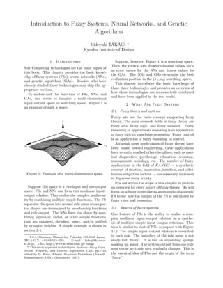
1. Introduction to Fuzzy Systems, Neural Networks, and Genetic
Algorithms
Hideyuki TAKAGI ∗
Kyushu Institute of Design
1 Introduction Suppose, however, Figure 1 is a searching space.
Then, the vertical axis shows evaluation values, such
Soft Computing technologies are the main topics of
as error values for the NNs and fitness values for
this book. This chapter provides the basic knowl-
the GAs. The NNs and GAs determine the best
edge of fuzzy systems (FSs), neural networks (NNs),
evaluation position in the (x 1 , x2) searching space.
and genetic algorithms (GAs). Readers who have
already studied these technologies may skip the ap- This chapter introduces the basic knowledge of
propriate sections. these three technologies and provides an overview of
how these technologies are cooperatively combined
To understand the functions of FSs, NNs, and
and have been applied in the real world.
GAs, one needs to imagine a multi-dimensional
input–output space or searching space. Figure 1 is 2 What Are Fuzzy Systems
an example of such a space.
2.1 Fuzzy theory and systems
Fuzzy sets are the basic concept supporting fuzzy
y theory. The main research fields in fuzzy theory are
fuzzy sets, fuzzy logic, and fuzzy measure. Fuzzy
reasoning or approximate reasoning is an application
of fuzzy logic to knowledge processing. Fuzzy control
is an application of fuzzy reasoning to control.
x2 Although most applications of fuzzy theory have
x1
been biased toward engineering, these applications
have recently reached other disciplines, such as med-
ical diagnostics, psychology, education, economy,
management, sociology, etc. The number of fuzzy
applications in the field of KANSEI — a synthetic
concept of emotion, impression, intuition, and other
Figure 1: Example of a multi-dimensional space. human subjective factors — has especially increased
in Japanese fuzzy society.
It is not within the scope of this chapter to provide
Suppose this space is a two-input and one-output an overview for every aspect of fuzzy theory. We will
space. FSs and NNs can form this nonlinear input– focus on a fuzzy controller as an example of a simple
output relation. They realize the complex nonlinear- FS to see how the output of the FS is calculated by
ity by combining multiple simple functions. The FS fuzzy rules and reasoning.
separates the space into several rule areas whose par-
tial shapes are determined by membership functions 2.2 Aspects of fuzzy systems
and rule output. The NNs form the shape by com- One feature of FSs is the ability to realize a com-
bining sigmoidal, radial, or other simple functions plex nonlinear input–output relation as a synthe-
that are enlarged, shrinked, upset, and/or shifted sis of multiple simple input–output relations. This
by synaptic weights. A simple example is shown in idea is similar to that of NNs (compare with Figure
section 3.4. 11.) The simple input–output relation is described
∗
4-9-1, Shiobaru, Minami-ku, Fukuoka, 815-8540 Japan, in each rule. The boundary of the rule areas is not
TEL&FAX +81-92-553-4555, E-mail: takagi@kyushu- sharp but ‘fuzzy.’ It is like an expanding sponge
id.ac.jp, URL: http://www.kyuhsu-id.ac.jp/ takagi soaking up water. The system output from one rule
0 This artcle appeared in Intelligent Systems: Fuzzy Logic,
area to the next rule area gradually changes. This is
Neural Networks, and Genetic Algorithms, Ch.1, pp.1–33,
edited by D. Ruan, Kluwer Academic Publishers (Norwell, the essential idea of FSs and the origin of the term
Massachusetts, USA), (September, 1997). ‘fuzzy.’

2. Another feature of FSs is the ability to separate On the other hand, rule-based control does not
logic and fuzziness. Since conventional two-value utilize the target system in modeling but is based
logic-based systems cannot do this, their rules are on the behavior of a skilled human operator (Fig-
modified when either logic or fuzziness should be ure 2(b).) Although most skilled operators do not
changed. The FSs modify fuzzy rules when logic know the mathematical behavior of their target sys-
should be changed and modify membership func- tems, they can control their systems. For example, a
tions which define fuzziness when fuzziness should skilled taxi driver probably does not know the math-
be changed. ematical equations of car behavior when his/her taxi
Suppose that the performance of an inverted pen- turns to the right up an unpaved hill, but he/she can
dulum controller is imperfect. Define a and a as the
˙ still handle the car safely. A fuzzy logic controller
angle between a pole in right side and vertical line describes the control behavior of the skilled human
and its angular velocity, respectively. operator using IF–THEN type of fuzzy rules.
IF a is positive big and a is big, THEN move
˙
2.4 Design of antecedent parts
a car to the right quickly. and
IF a is negative small a is small, THEN move
˙ Designing antecedent parts means deciding how to
a car to the left slowly. partition an input space. Most rule-based systems
are correct logic, and you need not change the fuzzy assume that all input variables are independent and
rules themselves. Only the definition of fuzziness partition the input space of each variable (see Fig-
must be modified in this case: big, small, quickly, ure 3.) This assumption makes it easy to not only
slowly, and so on. On the other hand, two-value partition the input space but also interpret parti-
logic rules, such as tioned areas into linguistic rules. For example, the
IF 40◦ ≤ a ≤ 60◦ and 50◦ /s ≤ a ≤ 80◦ /s, THEN move
˙ rule of “IF temperature is A1 and humidity is A2 ,
a car with 0.5 m/s. or THEN ...” is easy to understand, because the vari-
IF −20◦ ≤ a ≤ −10◦ and 10◦ /s ≤ a ≤ 20◦ /s, THEN
˙ ables of temperature and humidity are separated.
move a car with −0.1 m/s. Some researchers propose multi-dimensional mem-
must be modified whenever the rules or the quanti- bership functions that aim for higher performance
tative definitions of angle, angular velocity, and car by avoiding the constraint of variable independence
speed are changed. instead of linguistic transparency.
The difference between crisp and fuzzy rule-based
2.3 Mathematical model-based control and systems is how the input space is partitioned (com-
rule-based control pare Figure 3(a) with (b).) The idea of FSs is based
To understand FSs, fuzzy logic control will be used on the premise that in our real analog world, change
as a simple example of the FSs in this and the follow- is not catastrophic but gradual in nature. Fuzzy sys-
ing sections. The task is to replace a skilled human tems, then, allow overlapping rule areas to shift from
operator in the Figure 2 with a controller. one control rule to another. The degree of this over-
lapping is defined by membership functions. The
gradual characteristics allow smooth fuzzy control.
target system target system
input 2
input 2
(a) (b) rule 3 rule 4 rule 5 rule 3 rule 4 rule 5
Figure 2: (a) Conventional control theory tries to
make a mathematical model of a target system. (b) rule 1 rule 2 rule 1 rule 2
Rule-based control tries to make a model of a skilled input 1 input 1
human operator. ( a) ( b)
Figure 3: Rule partition of an input space: (a) parti-
The mathematical model-based control approach tion for crisp rules and (b) partition for fuzzy rules.
is based on classic and modern control theory and is
designed to observe the characteristics of the target
system, construct its mathematical model, and build
a controller based on the model. The importance is 2.5 Design of consequent parts
placed on the target system and the human operator The next step following the partitioning of an input
is not a factor in the design (Figure 2(a).) space is deciding the control value of each rule area.
2

3. Fuzzy models are categorized into three models ac- for this purpose is called t-norm operator. There
cording to the expressions of consequent parts: are many operators in t−norm category. One of the
(1) Mamdani model: y=A most frequently used t−norm operators is an alge-
k
(A is a fuzzy number.) braic product: rule strength wi = j=1 µj (xj ). The
(2) TSK model: y = a 0 + ai x i min operator that Mamdani used in his first fuzzy
(ai is a constant, and xi is an input variable.) control is also frequently introduced in fuzzy text-
(3) simplified fuzzy model y = c books: rule strength wi = min(µj (xj )).
(c is a constant.) The final system output, y∗ , is calculated by
The Mamdani type of FS has a fuzzy variable weighting each rule output with the obtained rule
defined by a membership function in their conse- strength, wi : y∗ = wi yi / wi . Mamdani type
quents, such as y = big or y = negative small, of fuzzy controllers defuzzify the aggregated system
which was used in the first historical fuzzy control output and determine the final non-fuzzy control
[(Mamdani, 1974)]. Although it is more difficult to value.
analyze this type of FS than a FS whose consequents Figure 4 is an example of a simple FS that has
are numerically defined, it is easier for this FS to de- four fuzzy rules. The first rule is “IF x1 is small
scribe qualitative knowledge in the consequent parts. and x2 is small, THEN y = 3x1 + 2x2 − 4.” Sup-
The Mamdani type of FS seems to be suitable for pose there is an input vector: (x1 , x2 ) = (10., 0.5).
knowledge processing expert systems rather than for Then, membership values are calculated. The first
control expert systems. rule has membership values, 0.8 and 0.3, for the in-
The consequents of the put values. The second one has 0.8 and 1.0. If the
TSK (Takagi-Sugeno-Kang) models are expressed by algebra product is used as a t-norm operator, then
the linear combination of weighted input variables the rule strength of the first rule is 0.8 × 0.3 = 0.24.
[(Takagi&Sugeno, 1985)]. It is possible to expand The rule strengths of the second, third, and fourth
the linear combination to nonlinear combination of rules are 0.8, 1.0, and 0.3, respectively. If min op-
input variables; for example, fuzzy rules which have erator is used, the rule strength of the first rule is
NNs in their consequents [(Takagi&Hayashi, 1991)]. min(0.8, 0.3) = 0.3. The output of each rule for the
In this case, there is a tradeoff between system per- input vector, (10., 0.5), is 27, 23.5, −9, and −20.5,
formance and the transparency of rules. The TSK respectively. Therefore, the final system output, y∗ ,
models are frequently used in fuzzy control fields as is given as:
well as the following simplified fuzzy models.
The simplified fuzzy model has fuzzy rules whose wi yi
consequents are expressed by constant values. This y∗ =
wi
model is the special case of both the Mamdani type
of FSs and the TSK models. Even if each rule out- 0.24 × 27 + 0.8 × 23.5 + 1.0 × (−9) + 0.3 × (−20.5)
=
put is constant, the output of the whole FS is nonlin- 0.24 + 0.8 + 1.0 + 0.3
∼
= 4.33
ear, because the characteristics of membership func-
tions are embedded into the system output. The
biggest advantage of the simplified fuzzy models is
that the models are easy to design. It is reported
that this model is equvalent to Mamdani’s model
[(Mizumoto, 1996)]. input x1 = 10 input x2 = 0.5
2.6 Fuzzy reasoning and aggregation
Now that the IF and THEN parts have been de- 1 0.8 1
THEN y = 3x1 + 2x2 - 4
IF and 0.3
signed, the next stage is to determine the final sys- x1 x2
= 27
tem output from the designed multiple fuzzy rules. 1 1
0.8
There are two steps: (1) determination of rule IF and THEN y = 2x1 - 3x2 + 5
x1 x2
strengths and (2) aggregations of each rule output. = 23.5
1
The first step is to determine rule strengths, mean- IF and
1
THEN y = -x1 - 4x2 + 3
ing how active or reliable each rule is. Antecedents x1 x2
= -9
include multiple input variables: 1 1
IF and 0.3 THEN y = -2x1 + 5x2 - 3
IF x1 ∈ µ1 and x2 ∈ µ2 and ... x k ∈ µk , THEN ... x1 x2
= -20.5
In this case, one fuzzy rule has k membership val-
ues: µi (xi ) (i = 1, ..., k). We need to determine how Figure 4: Example aggregation of TSK model.
active a rule is, or its strength, from the k member-
ship values. The class of the fuzzy operators used
3

4. to other neurons
dendrite 1
from other neurons
w0
axon x1
w1
cell body
y
w2
x2
wn
synapse
xn
(a) (b)
Figure 5: A biological neuron and an artificial neuron model.
3 What Are Neural Networks back and feed-forward NNs. Learning algorithms
3.1 Analogy from biological neural networks are categorized into supervised learning and unsu-
pervised learning. This section provides an overview
A biological neuron consists of dendrite, a cell body, of these models and algorithms.
and an axon (Figure 5(a)). The connections between
the dendrite and the axons of other neurons are
called synapses. Electric pulses coming from other
neurons are translated into chemical information at
each synapse. The cell body inputs these pieces of
information and fires an electric pulse if the sum of
the inputs exceeds a certain threshold. The network
consisting of these neurons is a NN, the most essen-
tial part of our brain activity.
The main function of the biological neuron is to (a) (b)
output pulses according to the sum of multiple sig-
nals from other neurons with the characteristics of a Figure 6: (a) a feed-back neural network, and (b) a
pseudo-step function. The second function of the feed-forward neural network.
neuron is to change the transmission rate at the
synapses to optimize the whole network.
An artificial neuron model simulates multiple in- The feed-back networks are NNs that have con-
puts and one output, the switching function of nections between network outputs and some or all
input–output relation, and the adaptive synaptic other neuron units (see Figure 6(a).) Certain unit
weights (Figure 5(b)). The first neuron model pro- outputs in the figure are used as activated inputs
posed in 1943 used a step function for the switching to the network, and other unit outputs are used as
function [(McCulloch&Pitts, 1943)]. However, the network outputs.
perceptron [(Rosenblatt, 1958)] that is a NN consist- Due to the feed-back, there is no guarantee that
ing of this type of neuron has limited capability, be- the networks become stable. Some networks con-
cause of the constraints of binary on/off signals. To- verge to one stable point, other networks become
day, several continuous functions, such as sigmoidal limit-cycle, and others become chaotic or divergent.
or radial functions, are used as a neuron character- These characteristics are common to all non-linear
istic functions, which results higher performance of systems which have feed-back.
NNs. To guarantee stability, constraints on synaptic
Several learning algorithms that change the weights are introduced so that the dynamics of the
synaptic weights have been proposed. The combina- feed-back NN is expressed by the Lyapunov func-
tion of the artificial NNs and the learning algorithms tion. Concretely, a constraint of equivalent mutual
have been applied to several engineering purposes. connection weights of two units is implemented. The
Hopfield network is one such NNs.
3.2 Several types of artificial neural networks It is important to understand two aspects of the
Many NN models and learning algorithms have been Hopfield network: (1) Synaptic weights are deter-
proposed. Typical network structures include feed- mined by analytically solving constraints not by per-
4

5. forming an iterative learning process. The weights
are fixed during the Hopfield network runs. (2) Final
network outputs are obtained by running feed-back y = f (∑ wi xi )
networks for the solutions of an application task. 0.4 0.2 0.9
Another type of NN which is compared with the
feed-back type is a feed-forward type. The feed-
forward network is a filter which outputs the pro- w1 w2 wn
cessed input signal. Several algorithms determine
synaptic weights to make the outputs match the de- x1 x2 xn
sired result.
Supervised learning algorithms adjust synaptic (a) (b)
weights using input–output data to match the input–
output characteristics of a network to desired char- Figure 7: (a) Hebbian learning algorithms strength
acteristics. The most frequently used algorithm, the weight, wi when input, xi activates a neuron, y.
backpropagation algorithm, is explained in detail in (b) Competitive learning algorithms strength only
the next section. weights connected to the unit whose output is the
Unsupervised learning algorithms use the mecha- biggest.
nism that changes synaptic weight values according
to the input values to the network, unlike supervised
learning which changes the weights according to su-
pervised data for the output of the network. Since
the output characteristics are determined by the −1.5
NN itself, this mechanism is called self-organization.
Hebbian learning and competitive learning are rep- 0 .8 −2 Σ −0
.63
5
resentative of unsupervised learning algorithms. 0.687
2.1
1.5
A Hebbian learning algorithm increases a weight,
wi , between a neuron and an input,xi , if the neuron,
y, fires. Σ 0.67
0.5
4
515 −0.
∆wi = ayxi , 0.
0 .2 −0.3 Σ
where a is a learning rate. Any weights are strength-
ened if units connected with the weights are acti- 1.14
vated. Weights are normalized to prevent an infinite
increase in weights. Figure 8: Example data flow in a simple feed-forward
Competitive learning algorithms modify weights neural network.
to generate one unit with the greatest output. Some
variations of the algorithm also modify other weights
by lateral inhibition to suppress the outputs of other
units whose outputs are not the greatest. Since One of the most popular learning algorithms
only one unit becomes active as the winner of the which iteratively determines the weights of the feed-
competition, the unit or the network is called a forward NNs is the backpropagation algorithm. A
winner-take-all unit or network. Kohonen’s self- simple learning algorithm that modifies the weights
organization feature map, one of the most well- between output and hidden layers is called a delta
known competitive NNs, modifies the weights con- rule. The backpropagation algorithm is an extension
nected to the winner-take-all unit as: of the delta rule that can train the weights, not only
between output and hidden layers but also hidden
∆wi = a(xi − wi ), and input layers. Historically, several researchers
have proposed this idea independently: S. Amari in
where the sum of input vectors is supposed to be 1967, A. Bryson and Y-C. Ho in 1969, P. Werbos
normalized as 1. in 1974, D. Parker in 1984, etc. Eventually, Rumel-
hart, et al. and the PDP group developed practical
3.3 Feed-forward NN and the backpropagation techniques that gave us a powerful engineering tool
learning algorithm [(Rumelhart, et al., 1986)].
Signal flow of a feed-forward NN is unidirectional Let E be an error between the NN outputs, v3 ,
from input to output units. Figure 8 shows a nu- and supervised data, y. The number at superposi-
merical example of the data flow of a feed-forward tion means the layer number. Since NN outputs are
NN. changed when synaptic weights are modified, the E
5

6. must be a function of the synaptic weights w:
Nk
1 y13 3 3
E(w) = (vj − yj )2 .
3 y2 y3 supervised data
2 j=1
3
v13 3
v2 v3 output of NN
Supposed that, in Figure 1, the vertical axis is E
and the x1 ... x n axes are the weights, w1 ... w n . output layer
w3,,13
2
Then, NN learning is to find the global minimum d j3 = (v 3 − y j )(1 − v 3 )v 3
 j j j
w12,13
,
w3,,33
2
coordinate in the surface of the figure.  2,3 3 2
∆wi , j = −εd j vi

Since E is a function of w, the searching direction
hidden layer(s)
of the smaller error point is obtained by calculating
w1,,12
1
w3,, 3
12 d j2 = Σ dh w 2,,h (1 − v 2 )v 2

3
j
3
j j
a partial differential. This technique is called the  1, 2
h =1
2 1
gradient method, and the steepest decent method ∆wi , j = −εd j vi

is the base of the backpropagation algorithm. The
searching direction, g = −∂E(w)/∂w, and modifi- Figure 9: Visual-aid of understanding the program-
cation of weights is given as ∆w = g. From this ming backpropagation algorithm.
equation, we finally obtain the following backpropa-
gation algorithm.
k−1,k k−1
∆wi,j = − dk vi
j
layer. For example, the unit (b1) has the synaptic
 (v3 − y ) ∂f (Uj )
k weight of −22.3 and −16.1 between the unit and the
 j j k for output layer input layer and outputs f() whose input is −22.3x −
∂Uj
dk =
j k

 Nk+1 k+1 k,k+1 ∂f (Uj ) 16.1.
h=1 dj wi,h ∂U k for hidden layer(s),
j One can understand how the NN forms the final
k−1,k output characteristics visually when the four out-
where wi,j is the connection weight between the puts of the hidden layer units with the final output
i-th unit in the (k − 1)-th layer and the j-th unit in characteristics are displayed (see Figure 11(c1) and
k
the k-th layer, and Uj is the total amount of input (c2).) The output characteristics of the NN consist
to the j-th unit at k-th layer. of four sigmoidal functions whose amplitudes and
To calculate dk , dk+1 must be previously calcu- center positions are changed by synaptic weights.
j j
lated. Since the calculation must be conducted in Thus, NNs can form any nonlinear function with any
the order of the direction from the output layer to precision by theoretically increasing the number of
input layer, this algorithm is named the backpropa- hidden units. It is important to note that a learning
gation algorithm. algorithm cannot always determine the best combi-
When a sigmoidal function is used for the charac- nation of weights.
teristic function, f(), of neuron units, the calculation
of the algorithm becomes simple. 4 What Are Genetic Algorithms
1 4.1 Evolutionary computation
f(x) = 1+exp−x+T
∂f (x)
= (1 − f(x))f(x) Searching or optimizing algorithms inspired by bi-
∂x
ological evolution are called evolutionary computa-
Figure 9 illustrates the backpropagation algorithm.
3.4 Function approximation
The following analysis of a simple NN that has
one input, four hidden nodes, and one output will y
demonstrate how NNs approximate the nonlinear re-
lationship between input and outputs (Figure 10.)
The ‘1’s in the figure are offset terms.
Figure 11(a1) – (a5) shows the input–output char-
acteristics of a simple NN during a training epoch, 1
where triangular points are trained data, and hori-
zontal and virtual axes are input and output ones.
After 480 iterations of training, the NN has learned x 1
the nonlinear function that passes through all train-
ing data points. Figure 10: Simple neural network to analyze nonlin-
As a model of the inside of the NN, Figure 11(b1) ear function approximation.
– (b4) shows the output of four units in the hidden
6

7. (a1) (b1) (c1)
(a2) (c2)
(b2)
(a3) (b3)
(a4) (b4)
(a5)
Figure 11: Analysis of NN inside. Triangular points are training data, and horizontal and virtual axes are
input and output axes. (a1) – (a5) are the input–output characteristics of a NN with the training of 10,
100, 200, 400, and 500 iterations, respectively. (b1) – (b4), the characteristics of four trained sigmoidal
functions in a hidden layer, are f(−22.3x − 16.1), f(−1.49x − 0.9), f(−20.7x + 10.3), and f(−21.5x + 4.9),
respectively; where w1 x + w0 is trained weights, wi , and input variable, x. (c1) is the same as (a5): the
input–output characteristics of the trained NN. (c2) is the overlapped display of (b1) – (b4). Comparison of
(c1) and (c2) shows the final NN input–output characteristics are formed by combining sigmoidal functions
inside with weighting the function.
tions. The features of the evolutionary computa- by adding Gaussian noise, and ES controls the pa-
tion are that its search or optimization is conducted rameters of a Gaussian distribution allowing it to
(1) based on multiple searching points or solution converge to a global optimum.
candidates (population based search), (2) using op- EPs are similar to GAs. The primary difference
erations inspired by biological evolution, such as is that mutation is the only EP operator. EPs use
crossover and mutation, (3) based on probabilistic real number coding, and the mutation sometimes
search and probabilistic operations, and (4) using changes the structure (length) of EP code. It is
little information of searching space, such as differ- said that the similarities and differences come from
ential information mentioned in section 3.3. Typical their background; GAs started from the simulation
paradigms which consist of the evolutionary com- of genetic evolution, while EPs started from that of
putation include GA (genetic algorithm), ES (evo- environmental evolution.
lution strategies), EP (evolutionary programming),
GPs use tree structure coding to represent a com-
and GP (genetic programming).
puter program or create new structures of tasks.
GAs usually represent solutions for chromosomes The crossover operation is not for a numerical value
with bit coding (genotype) and searches for the bet- but for a branch of the tree structure. Consider
ter solution candidates in the genotype space using the application’s relationship with NNs. GAs and
GA operations of selection, crossover, and mutation. ESs determine the best synaptic weights, which is
The crossover operation is the dominant operator. NN learning. GP, however, determines the best NN
ESs represent solutions as expressed by the chro- structure, which is a NN configuration.
mosomes with real number coding (phenotype) and It is beyond the scope of this chapter to describe
searches for the better solution in the phenotype these paradigms. We will focus only on GAs in the
space using the ES operations of crossover and mu- following sections and see how the GA searches for
tation. The mutation of a real number is realized solutions.
7

8. Table 1: Technical terms used in GA literatures
chromosome vector which represents solutions of application task
gene each solution which consists of a chromosome
selection choosing parents’ or offsprings’ chromosomes for the next generation
individual each solution vector which is each chromosome
population total individuals
population size the number of chromosome
fitness function a function which evaluates how each solution suitable to the given task
phenotype expression type of solution values in task world, for example, ‘red,’ “13 cm”, “45.2 kg”
genotype bit expression type of solution values used in GA search space, for example, “011,”
“01101.”
4.2 GA as a searching method expression. The solution expression of the bit code is
It is important to be acquainted with the technical decoded to values used in an application task. This
terms of GAs. Table 1 lists some of the terms fre- is phenotype expression. The multiple possible so-
quently used. lutions are applied to the application task and eval-
uated by each. These evaluation values are fitness
There are advantages and one distinct disadvan-
values. GA feed-backs the fitness values and selects
tage to using GAs as a search method.
current possible solutions according to their fitness
The advantages are: (1) fast convergence to near
values. They are parent solutions that determine
global optimum, (2) superior global searching ca-
the next searching points. This idea is based on the
pability in the space which has complex searching
expectation that better parents can probabilistically
surface, and (3) applicability to the searching space
generate better offspring. The offspring in the next
where we cannot use gradient information of the
generation are generated by applying the GA opera-
space.
tions, crossover and mutation, to the selected parent
The first and second advantages originate in
solution. This process is iterated until the GA search
population-based searching. Figure 12 shows this
converges to the required searching level.
situation. The gradient method determines the next
The GA operations are explained in the following
searching point using the gradient information at the
sections.
current searching point. On the other hand, the GA
determines the multiple next searching points using 4.4 GA operation: selection
the evaluation values of multiple current searching
points. When only the gradient information is used, Selection is an operation to choose parent solutions.
the next searching point is strongly influenced by the New solution vectors in the next generation are cal-
local geometric information of the current searching culated from them.
points. Sometimes it results in the searching be- Since it is expected that better parents generate
ing trapped at a local minima (see Figure 12.) On better offspring, parent solution vectors which have
the contrary, the GA determines the next searching higher fitness values have a higher probability to be
points using the fitness values of the current search- selected.
ing points which are widely spread throughout the There are several selection methods. Roulette
searching space, and it has the mutation operator wheel selection is a typical selection method. The
to escape from a local minima. This is why these probability to be a winner is proportional to the area
advantages are realized. rate of a chosen number on a roulette wheel. From
The key disadvantage of the GAs is that its con- this analogy, the roulette wheel selection gives the
vergence speed near the global optimum becomes selection probability to individuals in proportion to
slow. The GA search is not based on gradient infor- their fitness values.
mation but GA operations. There are several pro- The scale of fitness values is not always suitable
posals to combine the two searching methods. for the scale of selection probability. Suppose there
are a few individuals whose fitness values are very
4.3 GA operations high, and others whose are very low. Then, the few
Figs. 13 and 14 show the flows of GA process and parents are almost always selected and the variety of
data, respectively. Six possible solutions are ex- their offspring becomes small, which results in con-
pressed in bit code in Figure 14. This is the genotype vergence to a local minimum. Rank-based selection
8

9. GA
1st generation 3rd generation 5th generation
gradient
method
1st generation 3rd generation
Figure 12: GA search and gradient-based search.
uses an order scale of fitness values instead of a dis- have different bit at a certain bit position, then a
tance scale. For example, it gives the selection prov- complement bit of the poor parent is copied to the
ability of (100, 95, 90, 85, 80, ...) for the fitness values offspring. This is analogous to learning something
of (98, 84, 83, 41, 36, ...). from bad behavior. The left end bit of the example
Since the scales of fitness and selection are differ- in Figure 15 is the former case, and the second left
ent, scaling is needed to calculate selection proba- bit is the latter case.
bilities from fitness values. The rank-based selection
can be called linear scaling. There are several scaling 4.6 GA operation: mutation
methods, and the scaling influences GA conversion. When parent chromosomes have similar bit patterns,
Elitist strategy is an approach that copies the best the distance between the parents and offspring cre-
n parents into the next generation as they are. The ated by crossover is close in a genotype space. This
fitness value of offspring does not always become bet- means that the crossover cannot escape from the lo-
ter than those of its parents. The elitist strategy cal minimum if individuals are concentrated near the
prevents the best fitness value in the offspring gen- local minimum. If the parents in Figure 16 are only
eration from becoming worse than that in the previ- the black and white circles, offspring obtained by
ous generation by copying the best parent(s) to the combining bit strings of any of these parents will be
offspring. located nearby.
Mutation is an operation to avoid this trapping at
4.5 GA operation: crossover a local area by exchanging bits of chromosome. Sup-
Crossover is an operation to combine multiple par- pose the white individual jumps to the gray point in
ents and make offspring. The crossover is the the figure. Then, the searching area of GA spreads
most essential operation in GA. There are several widely. The mutated point has the second highest
ways to combine parent chromosomes. The simplest fitness value in the figure. If the point that has
crossover is called one-point crossover. The parent the highest fitness value and the mutated gray point
chromosomes are cut at one point, and the cut parts are selected and mate, then the offspring can be ex-
are exchanged. Crossover that uses two cut points is pected to be close to the global optimum.
called two-point crossover. Their natural expansion If the mutation rate is too high, the GA searching
is called multi-point crossover or uniform crossover. becomes a random search, and it becomes difficult
Figure 15 shows these standard types of crossover. to quickly converge to the global optimum.
There are several variations of crossover. One
4.7 Example
unique crossover is called the simplex crossover
[(Bersini&Scront, 1992)]. The simplex crossover The knapsack problem provides a concrete image of
uses two better parents and one poor parent and GA applications and demonstrates how to use GAs.
makes one offspring (the bottom of Figure 15.) Figure 17 illustrates the knapsack problem and its
When both better parents have the same ‘0’ or ‘1’ GA coding. The knapsack problem is a task to
at a certain bit position, the offspring copies the bit find the optimum combination of goods whose total
into the same bit position. When better parents amount is the closest to the amount of the knapsack,
9

10. initializing individuals
parent 1 1 0 0 1 0 1 1 0 0 0 1 1 offspring 1
one point crossover
parent 2 0 1 0 0 1 1 0 1 0 1 0 1 offspring 2
evaluation
parent 1 1 0 0 1 0 1 1 0 0 0 1 1 offspring 1
two points crossover
selection of parents parent 2 0 1 0 0 1 1 0 1 0 1 0 1 offspring 2
crossover
parent 1 1 0 0 1 0 1 0 0 0 0 0 1 offspring 1
uniform crossover
parent 2 0 1 0 0 1 1 1 1 0 1 1 1 offspring 2
mutation (multi-points crossover)
template ○ ● ○ ○ ● ●
better parent 1 1 0 0 1 0 1
Figure 13: The flow
better parent 2 0 1 0 0 1 1 simplex crossover 1 0 0 1 1 1 offspring
of GA process.
poor parent 0 1 1 0 0 1
scaling Fitness function application Figure 15: Several variations of crossover.
task
GA Operations
(selection, crossover, mutation)
35 47 32 with low mutation rate
1 0 1 0 1 0 0 01 1
65 69 18
0 0 1 1 0 1 0 1 1 0 83 43 25
1 1 01 1 0 1 0 01 decode 76 39 14
01 1 0 1 0 1 0 1 0 62 19 15 1 0 1 1 0 1
01 0 0 1 1 0 1 1 0 64 32 28
chromosome (phenotype)
0 1 01 01 0 0 0 1
=
chromosome (genotype)
possible solutions for task
1 1 1 1 0 1
GA Engine
Figure 16: Effect and an example of mutation.
Figure 14: The flow of GA data.
5 Models and Applications of
Cooperative Systems
There are many types of cooperative models of FSs,
or to find the optimum combination of goods whose NNs, and GAs. This section categorizes these types
total value is the highest under the condition that of models and introduces some of their industrial
the total amount of goods is less than that of the applications. Readers interested in further study of
knapsack. Although the knapsack problem itself is practical applications should refer to detailed sur-
a toy task, there are several similar practical prob- vey articles in such references as [(Takagi, 1996),
lems such as the optimization of CPU load under a (Yen et al. eds., 1995)].
multi-processing OS.
5.1 Designing FSs using NN or GA
Since there are six goods in Figure 17 and the task NN-driven fuzzy reasoning is the first model that
is to decide which goods are input into the knapsack, applies an NN to design the membership func-
the chromosome consists of six genes with the length tions of an FS explicitly [(Hayashi&Takagi,1988),
of 1 bit. For example, the first chromosome in the
figure means to put A, D, and F into the knapsack.
Then, the fitness values of all chromosome are cal-
culated. The total volume of A, D, and F is 60, that
AB CDE F fitness value
of B, E, and F is 53, that of A, D, E, and F is 68, chromosome 1 1 0 0 1 0 1 60
and so on. The fitness values do not need to be the Volume V A C E
chromosome 2 0 1 0 0 1 1 53
chromosome 3 1 0 0 1 1 1 68
total volume itself, but the fitness function should B D F
be a function of the total volume of the input goods. chromosome n 0 0 1 1 0 1 26
Then, GA operations are applied to the chromosome
to make the next generation. When the best solu- Figure 17: Knapsack problem and example of GA
tion exceeds the required minimum condition, the coding.
searching iteration is ended.
10

11. IF scanned shape is THEN control A ORDER FORM
IF scanned shape is THEN control B ORDER FORM
...
VP-211 2
...
IF scanned shape is THEN control N
NF-215 1
NG-166 2
...
HL-321 3
...
control 20 rolls
...
to make plate flat
plate surface
of plate surface
scanned depth
time scanning NARA
point at
width direction time t
FAX FAX
Figure 18: Rolling mill control by fuzzy and neural
systems. Scanned pattern of plate surface is recog-
nized by an NN. The output value of the each output
unit of the NN is used as a rule strength for the cor- Figure 19: FAX OCR: hand-written character recog-
responding fuzzy rule. nition system for a FAX ordering system.
(Takagi&Hayashi, 1991)]. The purpose of this model some Korean consumer products since 1994. Some
is to design the entire shape of non-linear multi- of them are: cool air flow control of refrigerators;
dimensional membership functions with an NN. The slow motor control of washing machines to wash
outputs of the NN are the rule strengths of each rule wool and/or lingerie [(Kim et al., 1995)]; neuro-
which are a combination of membership values in fuzzy models for dish washers, rice cookers, and mi-
antecedents. crowave ovens to estimate the number of dishes, to
The Hitachi rolling mill uses the model to con- estimate the amount of rice, and to increase con-
trol 20 rolls that flatten iron, stainless steel, trol performance; and FSs for refrigerators, washing
and aluminum plates to a uniform thickness machines, and vacuum cleaners [(Shin et al., 1995)].
[(Nakajima et al., 1993)]. An NN inputs the These neuro-fuzzy systems and FSs are tuned by
scanned surface shape of plate reel and outputs the GAs.
similarity between the input shape pattern and stan-
dard template patterns (see Figure 18). Since there 5.2 NN configuration based on fuzzy rule base
is a fuzzy control rule for each standard surface pat- NARA is a structured NN construct based on the IF-
tern, the outputs of the NN indicate how each con- THEN fuzzy rule structure [(Takagi et al., 1992)].
trol rule is activated. Dealing with the NN outputs An a priori knowledge of tasks is described by fuzzy
as rule strengths of all fuzzy rules, each control value rules, and small sub-NNs are combined according to
is weighted, and the final control values of the 20 the rule structure. Since a priori knowledge of the
rolls are obtained to make plate flat at the scanned task is embedded into the NARA, the complexity of
line. the task can be reduced.
Another approach parameterizes an FS and NARA has been used for a FAX ordering system.
tunes the parameters to optimize the FS using an When electric shop retailers order products from a
NN [(Ichihashi&Watanabe, 1990)] or using a GA Matsushita Electric dealer, they write an order form
[(Karr et al., 1989)]. For example, the shape of a by hand and send it by FAX. The FAX machine at
triangular membership function is defined by three the dealer site passes the FAX image to the NARA.
parameters: left, center, and right. The consequent The NARA recognizes the hand-written characters
part is also parameterized. and sends character codes to the dealer’s delivery
The approach using an NN was applied to develop center (Figure 19).
several commercial products. The first neuro-fuzzy
consumer products were introduced to the Japanese 5.3 Combination of NN and FS
market in 1991. This is the type of Figure 20, and There are many consumer products which use both
some of the applications are listed in section 5.3. NN and FS in a combination of ways. Although
The approach using a GA has been applied to there are many possible combinations of the two sys-
11

12. as developing tool
(MATSUSHITA ELECTRIC)
FS FS FS
FS NN
NN NN NN
(a) (b) (c) (d)
Figure 20: Combination types of an FS and an NN: (a) independent use, (b) developing tool type, (c)
correcting output mechanism, and (d) cascade combination.
Figure 20(d) shows a cascade combination of an
temperature exposure lamp control FS and an NN where the output of the FS or NN
humidity
grid voltage control
becomes the input of another NN or FS. An electric
toner density
fan developed by Sanyo detects the location of its
image density of back groud bias voltage control
remote controller with three infrared sensors. The
image density of solid black
exposured image density
toner density control outputs from these sensors change the fan’s direc-
tion according to the user’s location. First, a FS es-
timates the distance between the electric fan and the
remote controller. Then, a NN estimates the angle
from the estimated distance and the sensor outputs.
This two-stage estimation was adopted because it
was found that the outputs of three sensors change
Figure 21: Photo copier whose fuzzy system is tuned according to the distance to the remote controller
by a neural network. even if the angle is same.
Oven ranges manufactured by Toshiba use the
same combination. An NN first estimates the ini-
tems, the four combinations shown in Figure 20 have tial temperature and the number of pieces of bread
been applied to actual products. See the reference from sensor information. Then an FS determines the
of [(Takagi, 1995)] for details on these consumer ap- optimum cooking time and power by inputting the
plications. outputs of the NN and other sensor information.
Figure 20(a) shows the case where one piece of Figure 22 shows an example of this cascade model
equipment uses the two systems for different pur- applied to the chemical industry. Toshiba applied
poses without mutual cooperation. For example, the model to recover expensive chemicals that are
some Japanese air conditioners use an FS to prevent used to make paper from chips at a pulp factory
a compressor from freezing in winter and use an NN [(Ozaki, 1994)]. The task is to control the tempera-
to estimate the index of comfort, the PMV (Predic- ture of the liquid waste and air (or oxygen) sent to a
tive Mean Vote) value [(Fanger,1970)] in ISO-7730, recovering boiler, deoxidize liquid waste, and recover
from six sensor outputs. sulfureted sodium effectively.
The model in Figure 20(b) uses the NN to opti- The shape of the pile in the recovering boiler in-
mize the parameters of the FS by minimizing the fluences the efficiency of the deoxidization, which,
error between the output of the FS and the given in turn, influences the performance of recovering the
specification. Figure 21 shows an example of actual sulfureted sodium. An NN is used to recognized the
applications of this model. This model has been shape of the pile from the edge image detected from
used to develop washing machines, vacuum clean- the CCD image and image processing. An FS de-
ers, rice cookers, clothes driers, dish washers, electric termines the control parameters for PID control by
thermo-flask, inductive heating cookers, oven toast- using sensor data from the recovering boiler and the
ers, kerosene fan heaters, refrigerators, electric fans, recognized shape pattern of the pile.
range-hoods, and photo copiers since 1991.
5.4 NN learning and configuration based on GA
Figure 20(c) shows a model where the output of an
FS is corrected by the output of an NN to increase One important trend in consumer electronics is
the precision of the final system output. This model the feature that adapts to the user environment
is implemented in washing machines manufactured or preference and customizes mass produced equip-
by Hitachi, Sanyo, and Toshiba, and oven ranges ment at the user end. An NN learning func-
manufactured by Sanyo. tion is the leading technology for this purpose.
12

13. pattern recognition
ON/OFF time pattern
photosynthetic rate
CO 2
of shape
GA (fitness value) NN
image
processing NN
FS water drainage
sensing data & supply
air & heat
recovering boiler control
heated liquid waste
PID controller
for Figure 24: Water control for a hydroponics system.
air
air & heat control
recovered
chemicals
CCD camera
5.5 NN-based fitness function for GA
Figure 22: Chemicals recycling system at a pulp fac- A GA is a searching method that multiple individu-
tory. An NN identifies the shape of the chemical pile als apply to a task and evaluate for the subsequent
from the edge image, and a fuzzy system determines search. If the multiple individuals are applied to an
the control values for air and heat control to recover on-line process in addition to the usual GA applica-
chemicals optimally. tions, the process situation changes before the best
GA individual is determined.
One solution is to design a simulator of the task
process and embed the simulator into a fitness func-
room temp. tion. An NN can then be used as a process simula-
outdoor temp. RCE type control
time ref. temp. tor, trained with the input-output data of the given
NN
reference temp. process.
A GA whose fitness function uses an NN as a sim-
ulator of plant growth was used in a hydroponics
system [(Morimoto et al., 1993)]. The hydroponics
GA
system controls the timing of water drainage and
supply to the target plant to maximize its photosyn-
remote key
warm/cool thetic rate. The simulation NN is trained using the
timing pattern as input data and the amount of CO 2
Figure 23: Temperature control by a RCE neural as output data. The amount of CO 2 is used as an
network controller designed by GA at the user end. alternative to the photosynthetic rate of the plant.
Timing patterns of water drainage and supply gener-
ated by the GA are applied to the pseudo-plant, the
trained NN, and evaluated according to how much
Japanese electric companies applied a single user- CO2 they create (Figure 24). The best timing pat-
trainable NN to (1) kerosene fan heaters that learn tern is selected through the simulation and applied
and estimate when their owners use the heater to the actual plant.
[(Morito et al., 1991)], and (2) refrigerators that
learn when their owners open the doors to pre-cool 6 Summary
frozen food [(Ohtsuka et al., 1992)]. This chapter introduced the basic concepts and con-
LG Electric developed an air conditioner that im- crete methodologies of fuzzy systems, neural net-
plemented a user-trainable NN trained by a GA works, and genetic algorithms to prepare the read-
[(Shin et al., 1995)]. The NNs in RCE’s air con- ers for the following chapters. Focus was placed on:
ditioners inputs room temperature, outdoor tem- (1) the similarities between the three technologies
perature, time, and user-set temperature, and out- through the common keyword of nonlinear relation-
puts control values to maintain the user-set tempera- ship in a multi-dimensional space visualized in Fig-
ture [(Reilly et al., 1982)]. Suppose a user wishes to ure 1 and (2) how to use these technologies at a
change the control to low to adapt to his/her prefer- practical or programming level.
ence. Then, a GA changes the characteristics of the Readers who are interested in studying these ap-
NN by changing the number of neurons and weights plications further should refer to the related tutorial
(see Figure 23). papers.
13

14. References [(Ohtsuka et al., 1992)] Ohtsuka, H., Suzuki, N., Mina-
[(Bersini&Scront, 1992)] Bersini, H. and Scront, G., “In gawa, R., and Sugimoto, Y. “Applications of In-
search of a good evolution-optimization crossover,” telligent Control Technology to Home Appliances,”
in Parallel Problem Solving from Nature, R. Man- Mitsubishi Electric Technical Report, Vol.66, No.7,
ner and B. Mandrick (eds.), pp.479–488, Elsevier pp.728–731 (1992) (in Japanese)
Science Publishers, (1992). [(Ozaki, 1994)] Ozaki, T., “Recovering boiler control at
[(Fanger,1970)] Fanger, P. O., “Thermal Comfort — a pulp factory,” Neuro-Fuzzy-AI Handbook, Ohm
Analysis and Application in Environmental Engi- Publisher, pp.1209–1217 (1994) (in Japanese)
neering,” McGraw-Hill (1970) [(Reilly et al., 1982)] Reilly, D.L., Cooper, L.N., and
[(Hayashi&Takagi,1988)] Hayashi,I. and Takagi, H., Elbaum, C., “A neural model for category learn-
“Formulation of Fuzzy Reasoning by Neural Net- ing,” Biological Cybernetics, Vol.45, No.1, pp.35–41
work,” 4th Fuzzy System Symposium of IFSA (1982)
Japan, pp.55–60 (May, 1988) (in Japanese) [(Rosenblatt, 1958)] Rosenblatt, F., “The perceptron:
[(Ichihashi&Watanabe, 1990)] Ichihashi, H. and Watan- a probabilistic model for information storage and
abe, T., “Learning control by fuzzy models using a organization in the brain,” Psychological Review,
simplified fuzzy reasoning,” J. of Japan Society for Vol.65, pp.386–408 (1958)
Fuzzy Theory and Systems, Vol.2, No.3, pp.429–437 [(Rumelhart, et al., 1986)] Rumelhart, D.E., McClel-
(1990) (in Japanese) land, J.L., and the PDP Research Group, Paral-
[(Karr et al., 1989)] Karr, C., Freeman, L., Meredith, lel distributed processing: explorations in the mi-
D., “Improved Fuzzy Process Control of Space- crostructure of cognition, Cambridge, MA: MIT
craft Autonomous Rendezvous Using a Genetic Al- Press (1986)
gorithm,” SPIE Conf. on Intelligent Control and [(Shin et al., 1995)] Shin, M.S., Lee, K.L., Lim, T.L.,
Adaptive Systems, pp.274–283 (Nov., 1989) and Wang, B.H., “Applications of evolutionary
[(Kim et al., 1995)] Kim, J.W., Ahn, L.S., and Yi, Y.S., computations at LG Electrics,” in Fuzzy Logic for
“Industrial applications of intelligent control at the Applications to Complex Systems, ed. by W.
Samsung Electric Co., – in the Home Appliance Chiang and J. Lee, World Scientific Publishing,
Devision –,” in Fuzzy Logic for the Applications to pp.483–488 (1995)
Complex Systems, ed. by W. Chiang and J. Lee, [(Takagi&Sugeno, 1985)] Takagi, T. and Sugeno, M.,
World Scientific Publishing, pp.478–482 (1995) “Fuzzy Identification of Systems and Its Applica-
[(McCulloch&Pitts, 1943)] McCulloch, W. S. and Pitts, tions to Modeling and Control,” IEEE Trans. SMC-
W. H., “A logical calculus of the ideas immanent in 15-1, pp.116–132 (1985)
nervous activity,” Bullet. Math. Biophysics, Vol.5, [(Takagi&Hayashi, 1991)] Takagi, H. and Hayashi, I.,
pp.115–133 (1943) “NN-driven Fuzzy Reasoning,” Int’l J. of approx-
[(Mamdani, 1974)] Mamdani, E. H., “Applications of imate Reasoning (Special Issue of IIZUKA’88), Vol.
fuzzy algorithms for control of simple dynamic 5, No.3, pp.191–212 (1991)
plant,” Proc. of IEEE, Vol. 121, No. 12, pp.1585–
[(Takagi et al., 1992)] Takagi, H., Suzuki, N., Kouda,
1588 (1974)
T., Kojima, Y., “Neural networks designed on Ap-
[(Mizumoto, 1996)] Mizumoto, M., “Product- proximate Reasoning Architecture,” IEEE Trans.
sum-gravity method = fuzzy singleton-type reason- on Neural Networks, Vol. 3, No. 5, pp.752–760
ing method = simplified fuzzy reasoning method,” (1992)
Fifth IEEE Int’l Conf. on Fuzzy Systems, New Or-
[(Takagi, 1995)] Takagi, H., “Applications of Neural
leans, USA, pp.2098–2102, (Sept., 1996)
Networks and Fuzzy Logic to Consumer Products,”
[(Morimoto et al., 1993)] Morimoto, T., Takeuchi, T., ed. by J. Yen, R. Langari, and L. Zadeh, in Indus-
and Hashimoto, Y., “Growth optimization of plant trial Applications of Fuzzy Control and Intelligent
by means of the hybrid system of genetic algorithm Systems, Ch.5, pp.93–106, IEEE Press, Piscataway,
and neural network,” Int’l Joint Conf. on Neu- NJ, USA (1995)
ral Networks (IJCNN-93-Nagoya), Nagoya, Japan,
[(Takagi, 1996)] Takagi, H., “Industrial and Commer-
Vol.3, pp.2979–2982 (Oct. 1993).
cial Applications of NN/FS/GA/Chaos in 1990s,”
[(Morito et al., 1991)] Morito, K., Sugimoto, M., Araki, Int’l Workshop on Soft Computing in Industry
T., Osawa, T., and Tajima, Y., “Kerosene fan (IWSCI’96), Muroran, Hokkaido, Japan, pp.160–
heater using fuzzy control and neural networks 165 (April, 1996)
CFH-A12JD ”, Sanyo Technical Review, Vol. 23,
No. 3, pp.93–100 (1991) (in Japanese) [(Yen et al. eds., 1995)] Yen, J., Langari, R., and Zadeh,
L., (edit.) Industrial Applications of Fuzzy Control
[(Nakajima et al., 1993)] Nakajima, M., Okada, T., and Intelligent Systems, IEEE Press, Piscataway,
Hattori, S., and Morooka, Y., “Application of pat- NJ, USA (1995)
tern recognition and control technique to shape con-
trol of the rolling mill,” Hitachi Review, Vol.75,
No.2, pp.9–12 (1993) (in Japanese)
14