computer notes - Avl tree

ecomputernotes.com Data Structures Lecture No. 20
___________________________________________________________________

Data Structures

Lecture No. 20

We will continue the discussion on AVL tree in this lecture. Before going ahead, it will
be better to recap things talked about in the previous lecture. We built a balanced
search tree (BST) with sorted data. The numbers put in that tree were in increasing
sorted order. The tree built in this way was like a linked list. It was witnessed that the
use of the tree data structure can help make the process of searches faster. We have
seen that in linked list or array, the searches are very time consuming. A loop is
executed from start of the list up to the end. Due to this fact, we started using tree data
structure. It was evident that in case, both the left and right sub-trees of a tree are
almost equal, a tree of n nodes will have log2 n levels. If we want to search an item in
this tree, the required result can be achieved, whether the item is found or not, at the
maximum in the log n comparisons. Suppose we have 100,000 items (number or
names) and have built a balanced search tree of these items. In 20 (i.e. log 100000)
comparisons, it will be possible to tell whether an item is there or not in these 100,000
items.

AVL Tree
In the year 1962, two Russian scientists, Adelson-Velskii and Landis, proposed the
criteria to save the binary search tree (BST) from its degenerate form. This was an
effort to propose the development of a balanced search tree by considering the height
as a standard. This tree is known as AVL tree. The name AVL is an acronym of the
names of these two scientists.
An AVL tree is identical to a BST, barring one difference i.e. the height of the left and
right sub-trees can differ by at most 1. Moreover, the height of an empty tree is
defined to be ( 1).
Keeping in mind the idea of the level of a tree, we can understand that if the root of a
tree is at level zero, its two children (subtrees) i.e. nodes will be at level 1. At level 2,
there will be 4 nodes in case of a complete binary tree. Similarly at level 3, the number
of nodes will be 8 and so on. As discussed earlier, in a complete binary tree, the
number of nodes at any level k will be 2k. We have also seen the level order traversal of
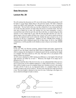
a tree. The term height is identical to the level of a tree. Following is the figure of a
tree in which level/height of nodes is shown.
level
5
-------------------------------- -----------
-- 0
2 8 ---------------------------
1

1 4 7 ----------------------------------
2
3 --------------------------------------------------------
----- 3 Page 1 of 11

Fig 20.1: levels of nodes in a tree

___________________________________________________________________

Here in the figure, the root node i.e. 5 is at the height zero. The next two nodes 2 and
8 are at height (or level) 1. Then the nodes 1, 4 and 7 are at height 2 i.e. two levels
below the root. At the last, the single node 3 is at level (height) 3. Looking at the
figure, we can say that the maximum height of the tree is 3. AVL states that a tree
should be formed in such a form that the difference of the heights (maximum no of
levels i.e. depth) of left and right sub-trees of a node should not be greater than 1. The
difference between the height of left subtree and height of right subtree is called the
balance of the node. In an AVL tree, the balance (also called balance factor) of a node
will be 1,0 or 1 depending on whether the height of its left subtree is greater than,
equal to or less than the height of its right subtree.
Now consider the tree in the figure 20.1. Its root node is 5. Now go to its left subtree
and find the deepest node in this subtree. We see that node 3 is at the deepest level.
The level of this deepest node is 3, which means the height of this left subtree is 3.
Now from node 5, go to its right subtree and find the deepest level of a node. The
node 7 is the deepest node in this right subtree and its level is 2. This means that the
height of right subtree is 2. Thus the difference of height of left subtree (i.e. 3) and
height of right subtree (i.e. 2) is 1. So according to the AVL definition, this tree is
balanced one. But we know that the AVL definition does not apply only to the root
node of the tree. Every node (non-leaf or leaf) should fulfill this definition. This means
that the balance of every node should be 1, 0 or 1. Otherwise, it will not be an AVL
tree.
Now consider the node 2 and apply the definition on it. Let s see the result. The left
subtree of node 2 has the node 1 at deepest level i.e. level 2. The node 2, itself, is at
level 1, so the height of the left subtree of node 2 is 2-1 i.e. 1. Now look at the right
subtree of node 2. The deepest level of this right subtree is 3 where the node 3 exists.
The height of this right subtree of node 2 will be 3 1 = 2 as the level of node 2 is 1.
Now the difference of the height of left subtree (i.e. 1) and height of the right subtree
(i.e. 2) is 1. We subtract the height of left subtree from the height of the right subtree
and see that node 2 also fulfills the AVL definition. Similarly we can see that all other
nodes of the tree (figure 20.1) fulfill the AVL definition. This means that the balance of
each node is 1, 0 or 1. Thus it is an AVL tree, also called the balanced tree. The
following figure shows the tree with the balance of each node.

level
1
5
---------------------------- ---------------
-- 0
-1 2 1 8 ---------------------------
1

0 1
1 4 0 7 --------------------------------- Page 2 of 11
2
0 3 --------------------------------------------------------

___________________________________________________________________

Let s consider a tree where the condition of an AVL tree is not being fulfilled. The
following figure shows such a tree in which the balance of a node (that is root node 6)
is greater than 1. In this case, we see that the left subtree of node 6 has height 3 as its
deepest nodes 3 and 5 are at level 3. Whereas the height of its right subtree is 1 as the
deepest node of right subtree is 8 i.e. level 1. Thus the difference of heights (i.e.
balance) is 2. But according to AVL definition, the balance should be1, 0 or 1. As
shown in the figure, this node 6 is only the node that violates the AVL definition (as its
balance is other than 1, 0 and -1). The other nodes fulfill the AVL definition. We know
that to be an AVL tree, each node of the tree should fulfill the definition. Here in this
tree, the node 6 violates this definition so this is not an AVL tree.

level
2
6
------------------------------------------
-0
-1 1 0 8 ---------------------------
1

0 1 0 4 ----------------------------------------------
-2
0 3 0 5 ------------------------------------
-3

Fig 20.3: not an AVL tree

From the above discussion, we encounter two terms i.e. height and balance which can
be defined as under.

Height
The height of a binary tree is the maximum level of its leaves. This is the same
definition as of depth of a tree.

Balance

Page 3 of 11

___________________________________________________________________
The balance of a node in a binary search tree is defined as the height of its left subtree
minus height of its right subtree. In other words, at a particular node, the difference in
heights of its left and right subtree gives the balance of the node.
The following figure shows a balanced tree. In this figure the balance of each node is
shown along with. We can see that each node has a balance 1, 0 or 1.

-1 6

0 12
1 4

1 -1 14
0 2 0 5 10

0 0 0
1 3 8 0 11 0 13 0 16

0 7 0 9 0 15 0 17

Fig 20.4: A balanced binary tree

Here in the figure, we see that the balance of the root (i.e. node 6) is 1. We can find
out this balance. The deepest level of the left subtree is 3 where the nodes 1 and 3 are
located. Thus the height of left subtree is 3. In the right subtree, we see some leaf
nodes at level 3 while some are found at level 4. But we know that the height of the
tree is the maximum level. So 4 is the height of the right subtree. Now we know that
the balance of the root node will be the result of height of left subtree minus the height
of right subtree. Thus the balance of the root node is 3 4 = -1. Similarly we can
confirm the balance of other nodes. The confirmation of balance of the other nodes of
the tree can be done. You should do it as an exercise. The process of height
computation should be understood as it is used for the insertion and deletion of nodes
in an AVL tree. We may come across a situation, when the tree does not remain
balanced due to insertion or deletion. For making it a balanced one, we have to carry
out the height computations.
While dealing with AVL trees, we have to keep the information of balance factor of
the nodes along with the data of nodes. Similarly, a programmer has to have additional
information (i.e. balance) of the nodes while writing code for AVL tree.

Insertion of Node in an AVL Tree
Now let s see the process of insertion in an AVL tree. We have to take care that the
tree should remain AVL tree after the insertion of new node(s) in it. We will now see
how an AVL tree is affected by the insertion of nodes.

Page 4 of 11

___________________________________________________________________
We have discussed the process of inserting a new node in a binary search tree in
previous lectures. To insert a node in a BST, we compare its data with the root node.
If the new data item is less than the root node item in a particular order, this data item
will hold its place in the left subtree of the root. Now we compare the new data item
with the root of this left subtree and decide its place. Thus at last, the new data item
becomes a leaf node at a proper place. After inserting the new data item, if we traverse
the tree with the inorder traversal, then that data item will become at its appropriate
position in the data items. To further understand the insertion process, let s consider
the tree of figure 20.4. The following figure (Fig 20.5) shows the same tree with the
difference that each node shows the balance along with the data item. We know that a
new node will be inserted as a leaf node. This will be inserted where the facility of
adding a node is available. In the figure, we have indicated the positions where a new
node can be added. We have used two labels B and U for different positions where a
node can be added. The label B indicates that if we add a node at this position, the tree
will remain balanced tree. On the other hand, the addition of a node at the position
labeled as U1, U2 .U12, the tree will become unbalanced. That means that at some
node the difference of heights of left and right subtree will become greater than 1.

-1 6

1 4 0 12

0 0 1 10 -1 14
2 5

B B
0 1 0 3 0 8 0 11 0 13 0 16

U1 U2 U3 B B B B
U4 0 7 0 9 0 15 0 17

U5 U6 U7 U8 U9 U10 U11
U12

Fig 20.5: Insertions and effect in a balanced tree

By looking at the labels B, U1, U2 .U12, we conclude some conditions that will
be implemented while writing the code for insert method of a balanced tree.
We may conclude that the tree becomes unbalanced only if the newly inserted node

• Is a left descendent of a node that previously had a balance of 1
(in the figure 20.5 these positions are U1, U2 ..U8)
• Or is a descendent of a node that previously had a balance of 1
(in the tree in fig 20.5 these positions are U9, U10, U11 and U12)

Page 5 of 11

___________________________________________________________________

The above conditions are obvious. The balance 1 of a node indicates that the height of
its left subtree is 1 more than the height of its right subtree. Now if we add a node to
this left subtree, it will increase the level of the tree by 1. Thus the difference of heights
will become 2. It violates the AVL rule, making the tree unbalanced.
Similarly the balance 1 of a node indicates that the right subtree of this node is one
level deep than the left subtree of the node. Now if the new node is added in the right
subtree, this right subtree will become deeper. Its depth/height will increase as a new
node is added at a new level that will increase the level of the tree and the height. Thus
the balance of the node, that previously has a balance 1, will become 2.
The following figure (Fig 20.6) depicts this rule. In this figure, we have associated the
new positions with their grand parent. The figure shows that U1, U2, U3 and U4 are
the left descendents of the node that has a balance 1. So according to the condition, the
insertion of new node at these positions will unbalance the tree. Similarly the positions
U5, U6, U7 and U8 are the left descendents of the node that has a balance 1.
Moreover we see that the positions U9, U10, U11 and U12 are the right descendents
of the node that has balance 1. So according to the second condition as stated earlier,
the insertion of a new node at these positions would unbalance the tree.

-1 6

0 12
1 4

1 -1 14
0 2 0 5 10

B B
0 0 0
1 3 8 0 11 0 13 0 16

U1 U2 U3 B B B B
U4 0 7 0 9 0 15 0 17

U5 U6 U7 U8 U9 U10 U11
U12

Fig 20.6: Insertions and effect in a balanced tree

Now let s discuss what should we do when the insertion of a node makes the tree
unbalanced. For this purpose, consider the node that has a balance 1 in the previous
tree. This is the root of the left subtree of the previous tree. This tree is shown as
shaded in the following figure.

-1 6

0 12
1 4
Page 6 of 11
1 -1 14
0 0 10
2 5

___________________________________________________________________

We will now focus our discussion on this left subtree of node having balance 1 before
applying it to other nodes. Look at the following figure (Fig 20.8). Here we are talking
about the tree that has a node with balance 1 as the root. We did not mention the other
part of the tree. We indicate the root node of this left subtree with label A. It has
balance 1. The label B mentions the first node of its left subtree. Here we did not
mention other nodes individually. Rather, we show a triangle that depicts all the nodes
in subtrees. The triangle T3 encloses the right subtree of the node A. We are not
concerned about the number of nodes in it. The triangles T1 and T2 mention the left
and right subtree of the B node respectively. The balance of node B is 0 that describes
that its left and right subtrees are at same height. This is also shown in the figure.
Similarly we see that the balance of node A is 1 i.e. its left subtree is one level deep
than its right subtree. The dotted lines in the figure show that the difference of
depth/height of left and right subtree of node A is 1 and that is the balance of node A.

A 1

B 0

T3

1
T1 T2

Fig 20.8: Inserting new node in AVL tree

Page 7 of 11

___________________________________________________________________
Now considering the notations of figure 20.8, let s insert a new node in this tree and
observe the effect of this insertion in the tree. The new node can be inserted in the tree
T1, T2 or T3. We suppose that the new node goes to the tree T1. We know that this
new node will not replace any node in the tree. Rather, it will be added as a leaf node
at the next level in this tree (T1). The following figure (fig 20.9) shows this
phenomenon.

A 2

B 1

T3

1
T1 T2
2

new

Fig 20.9: Inserting new node in AVL tree

Due to the increase of level in T1, its difference with the right subtree of node A (i.e.
T3) will become 2. This is shown with the help of dotted line in the above figure. This
difference will affect the balances of node A and B. Now the balance of node A
becomes 2 while balance of node B becomes 1. These new balances are also shown in
the figure. Now due to the balance of node A (that is 2), the AVL condition has been
violated. This condition states that in an AVL tree the balance of a node cannot be
other than 1, 0 or 1. Thus the tree in fig 20.9 is not a balanced (AVL) tree.
Now the question arises what a programmer should do in case of violation of AVL
condition .In case of a binary search tree, we insert the data in a particular order. So
that at any time if we traverse the tree with inorder traversal, only sorted data could be
obtained. The order of the data depends on its nature. For example, if the data is
numbers, these may be in ascending order. If we are storing letters, then A is less than
B and B is less than C. Thus the letters are generally in the order A, B, C . This
order of letters is called lexographic order. Our dictionaries and lists of names follow
this order.
If we want that the inorder traversal of the tree should give us the sorted data, it will
not be necessary that the nodes of these data items in the tree should be at particular
positions. While building a tree, two things should be kept in mind. Firstly, the tree
should be a binary tree. Secondly, its inorder traversal should give the data in a sorted
order. Adelson-Velskii and Landis considered these two points. They said that if we
see that after insertion, the tree is going to be unbalanced. Then the things should be

Page 8 of 11

___________________________________________________________________
reorganized in such a way that the balance of nodes should fulfill the AVL condition.
But the inorder traversal should remain the same.
Now let s see the example of tree in figure 20.9 and look what we should do to
balance the tree in such a way that the inorder traversal of the tree remains the same.
We have seen in figure 20.9 that the new node is inserted in the tree T1 as a new leaf
node. Thus T1has been modified and its level is increased by 1. Now due to this, the
difference of T1 and T3 is 2. This difference is the balance of node A as T1 and T3 are
its left and right subtrees respectively. The inorder traversal of this tree gives us the
result as given below.

T1 B T2 A T3

Now we rearrange the tree and it is shown in the following figure i.e. Fig 20.10.

B 0

A
0

T1

T2 T3

Fig 20.10: Rearranged tree after inserting a new
node

By observing the tree in the above figure we notice at first that node A is no longer the
root of the tree. Now Node B is the root. Secondly, we see that the tree T2 that was
the right subtree of B has become the left subtree of A. However, tree T3 is still the
right subtree of A. The node A has become the right subtree of B. This tree is balanced
with respect to node A and B. The balance of A is 0 as T2 and T3 are at the same
level. The level of T1 has increased due to the insertion of new node. It is now at the
same level as that of T2 and T3. Thus the balance of B is also 0. The important thing in
this modified tree is that the inorder traversal of it is the same as in the previous tree
(fig 10.9) and is

T1 B T2 A T3

We see that the above two trees give us data items in the same order by inorder
traversal. So it is not necessary that data items in a tree should be in a particular node
at a particular position. This process of tree modification is called rotation.

Page 9 of 11

___________________________________________________________________
Example (AVL Tree Building)
Let s build an AVL tree as an example. We will insert the numbers and take care of the
balance of nodes after each insertion. While inserting a node, if the balance of a node
becomes greater than 1 (that means tree becomes unbalance), we will rearrange the
tree so that it should become balanced again. Let s see this process.
Assume that we have insert routine (we will write its code later) that takes a data item
as an argument and inserts it as a new node in the tree. Now for the first node, let s say
we call insert (1). So there is one node in the tree i.e. 1. Next, we call insert (2). We
know that while inserting a new data item in a binary search tree, if the new data item
is greater than the existing node, it will go to the right subtree. Otherwise, it will go to
the left subtree. In the call to insert method, we are passing 2 to it. This data item i.e. 2
is greater than 1. So it will become the right subtree of 1 as shown below.

1

2

As there are only two nodes in the tree, there is no problem of balance yet.
Now insert the number 3 in the tree by calling insert (3). We compare the number 3
with the root i.e.1. This comparison results that 3 will go to the right subtree of 1. In
the right subtree of 1 there becomes 2. The comparison of 3 with it results that 3 will
go to the right subtree of 2. There is no subtree of 2, so 3 will become the right subtree
of 2. This is shown in the following figure.

1 -2

2

3

Let s see the balance of nodes at this stage. We see that node 1 is at level 0 (as it is the
root node). The nodes 2 and 3 are at level 1 and 2 respectively. So with respect to the
node 1, the deepest level (height) of its right subtree is 2. As there is no left subtree of
node 1 the level of left subtree of 1 is 0. The difference of the heights of left and right
subtree of 1 is 2 and that is its balance. So here at node 1, the AVL condition has
been violated. We will not insert a new node at this time. First we will do the rotation
to make the tree (up to this step) balanced. In the process of inserting nodes, we will
do the rotation before inserting next node at the points where the AVL condition is
being violated. We have to identify some things for doing rotation. We have to see that
on what nodes this rotation will be applied. That means what nodes will be rearranged.
Some times, it is obvious that at what nodes the rotation should be done. But there
may situations, when the things will not be that clear. We will see these things with the
help of some examples.

Page 10 of 11

___________________________________________________________________
In the example under consideration, we apply the rotation at nodes1 and 2. We rotate
these nodes to the left and thus the node 1 (along with any tree if were associated with
it) becomes down and node 2 gets up. The node 3 (and trees associated with it, here is
no tree as it is leaf node) goes one level upward. Now 2 is the root node of the tree
and 1 and 3 are its left and right subtrees respectively as shown in the following figure.

1 -2
2

2

1 3
3

Non AVL Tree AVL tree after applying rotation

We see that after the rotation, the tree has become balanced. The figure reflects that
the balance of node 1, 2 and 3 is 0. We see that the inorder traversal of the above tree
before rotation (tree on left hand side) is 1 2 3. Now if we traverse the tree after
rotation (tree on right hand side) by inorder traversal, it is also 1 2 3. With respect to
the inorder traversal, both the traversals are same. So we observe that the position of
nodes in a tree does not matter as long as the inorder traversal remains the same. We
have seen this in the above figure where two different trees give the same inorder
traversal. In the same way we can insert more nodes to the tree. After inserting a node
we will check the balance of nodes whether it violates the AVL condition. If the tree,
after inserting a node, becomes unbalance then we will apply rotation to make it
balance. In this way we can build a tree of any number of nodes.

Page 11 of 11

computer notes - Avl tree

Recomendados

Recomendados

Mais conteúdo relacionado

Mais de ecomputernotes

Mais de ecomputernotes (20)

Último

Último (20)

computer notes - Avl tree