
Recomendados
Mais conteúdo relacionado
Mais procurados
Mais procurados (9)
Semelhante a Creating Profiling Tools to Analyze and Optimize FiPy Presentation
Semelhante a Creating Profiling Tools to Analyze and Optimize FiPy Presentation (20)
Último
Último (20)
Creating Profiling Tools to Analyze and Optimize FiPy Presentation
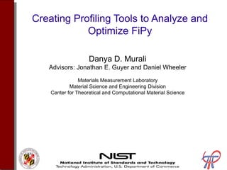
- 1. Creating Profiling Tools to Analyze and Optimize FiPy Danya D. Murali Advisors: Jonathan E. Guyer and Daniel Wheeler Materials Measurement Laboratory Material Science and Engineering Division Center for Theoretical and Computational Material Science
- 2. Outline ● FiPy Introduction ● How it works ● Examples ● Problems with FiPy ● Profiling Tools ● What are the they? ● How our tools work ● Results ● Conclusion
- 3. What is FiPy? ● An open source Python-based program that uses the Finite Volume method to numerically solve Partial Differential Equations (PDEs) ● Python has many powerful numerical libraries ● Designed for material scientists by material scientists
- 4. What is a PDE?
- 5. Finite Volume Method ● Solve a general PDE on a given domain for a field
- 6. Finite Volume Method ● Solve a general PDE on a given domain for a field ● Integrate PDE over general control volumes
- 7. Finite Volume Method ● Solve a general PDE on a given domain for a field ● Integrate PDE over general control volumes ● Integrate PDE over polyhedral control volumes
- 8. Finite Volume Method ● Solve a general PDE on a given domain for a field ● Integrate PDE over general control volumes ● Integrate PDE over polyhedral control volumes ● Obtain a set of linear equations
- 9. How FiPy Works import fipy as fp L = 1. N = 100 m = fp.Grid2D(Lx=L, Ly=L, nx=N, ny=N) v = fp.CellVariable(mesh=m) x, y = m.cellCenters v[x > L / 2] = 1. v.constrain(0., where=m.facesLeft | m.facesRight) v.constrain(1., where=m.facesTop | m.facesBottom) e = fp.TransientTerm() == fp.DiffusionTerm() for i in range(10): e.solve(v, dt=0.001) fp.Viewer(v).plot()
- 10. How FiPy Works import fipy as fp L = 1. N = 100 m = fp.Grid2D(Lx=L, Ly=L, nx=N, ny=N) v = fp.CellVariable(mesh=m) x, y = m.cellCenters v[x > L / 2] = 1. v.constrain(0., where=m.facesLeft | m.facesRight) v.constrain(1., where=m.facesTop | m.facesBottom) e = fp.TransientTerm() == fp.DiffusionTerm() for i in range(10): e.solve(v, dt=0.001) fp.Viewer(v).plot()
- 11. Examples of FiPy: Polycrystal and Phase Field courtesy S. A. David, ORNL
- 12. courtesy S. A. David, ORNL Examples of FiPy: Polycrystal and Phase Field
- 13. courtesy S. A. David, ORNL Examples of FiPy: Polycrystal and Phase Field heatEq = (TransientTerm(var=dT) == DiffusionTerm(coeff=Dt, var=dT) + TransientTerm(var=phase)) psi = theta + arctan2(phase.faceGrad[1], phase.faceGrad[0]) Phi = tan(N * psi / 2) PhiSq = Phi**2 beta = (1. - PhiSq) / (1. + PhiSq) DbetaDpsi = -N * 2 * Phi / (1 + PhiSq) Ddia = (1.+ c * beta) Doff = c * DbetaDpsi D = alpha**2 * (1.+ c * beta) * (Ddia * (( 1, 0), ( 0, 1)) + Doff * (( 0,-1), ( 1, 0))) phaseEq = (TransientTerm(coeff=tau, var=phase) == DiffusionTerm(coeff=D, var=phase) + ImplicitSourceTerm(coeff=(phase - 0.5 - kappa1 / pi * arctan(kappa2 * dT)) * (1 - phase)), var=phase) eq = heatEq & phaseEq
- 14. courtesy S. A. David, ORNL Examples of FiPy: Polycrystal and Phase Field
- 15. Examples Of FiPy: Extreme Fill
- 16. Examples Of FiPy: Extreme Fill adsorptionCoeff = dt * suppressor * kPlus thetaEq = fp.TransientTerm() == fp.ExplicitUpwindConvectionTerm(fp.SurfactantConvectionVariable(di stance)) + adsorptionCoeff * surface - fp.ImplicitSourceTerm(adsorptionCoeff * distance._cellInterfaceFlag) - fp.ImplicitSourceTerm(kMinus * depositionRate * dt)
- 17. Examples Of FiPy: Extreme Fill
- 18. Problems with FiPy ● Potentially time inefficient and excessive in memory usage ● But how do we measure that? ● Why do we even care? ● How do we find the bottlenecks? ● Need profiling tools!
- 19. Profiling Tools ● What is profiling? ● Tool used to identify and quantify what resources are being used by certain parts of a program
- 20. Profiling Tools ● What is profiling? ● Tool used to identify and quantify what resources are being used by certain parts of a program ● Our profiler needs to:
- 21. Profiling Tools ● What is profiling? ● Tool used to identify and quantify what resources are being used by certain parts of a program ● Our profiler needs to: ● Profile multiple functions at once
- 22. Profiling Tools ● What is profiling? ● Tool used to identify and quantify what resources are being used by certain parts of a program ● Our profiler needs to: ● Profile multiple functions at once ● Cache profiling data for many simulations
- 23. Profiling Tools ● What is profiling? ● Tool used to identify and quantify what resources are being used by certain parts of a program ● Our profiler needs to: ● Profile multiple functions at once ● Cache profiling data for many simulations ● Produce graphs of performance scaling against system size
- 24. Speed Profiling class FiPyProfileTime(FiPyProfile): def __init__(self, profileFunc, ncells, regenerate=False): ... def profile(self, ncell): ... def get_time_for_function(self, function_key): return stats[function_key] def get_key_from_function_pointer(function_pointer): return inspect.getfile(function_pointer) def plot(self, keys, field="cumulative"): ...
- 25. Memory Profiling class MemoryProfiler(object): def __init__(self, profileMethod, runfunc): ... def decorate(self, func): def wrapper(*args, **kwargs): ... return self.codeMap def getLineMemory(self, line): ... class MemoryViewer(object): def generateData(self): def worker(ncell, resultQ, profileMethod, runfunc, lines): process = multiprocessing.Process(...)
- 26. Results: Profiling Polycrystal - Memory
- 27. Results: Profiling Polycrystal - Speed
- 28. Results: Profiling Extreme Fill - Memory
- 29. Results: Profiling Extreme Fill - Speed
- 30. Results: Profiling Different Solvers
- 31. So What? ● Identified that FiPy has memory issues that need to be addressed ● Limits the size of simulations that we can run ● Located the classic memory for speed trade off with Gmsh ● Determined that using inline was faster ● Identified that Trilinos is much slower than Pysparse but has the option to run in parallel ● Next Step: Analyze algorithms to figure out how to address these issues
- 32. So What? ● Identified that FiPy has memory issues that need to be addressed ● Limits the size of simulations that we can run ● Located the classic memory for speed trade off with Gmsh ● Determined that using inline was faster ● Identified that Trilinos is much slower than Pysparse but has the option to run in parallel ● Next Step: Analyze algorithms to figure out how to address these issues
- 33. So What? ● Identified that FiPy has memory issues that need to be addressed ● Limits the size of simulations that we can run ● Located the classic memory for speed trade off with Gmsh ● Determined that using inline was faster ● Identified that Trilinos is much slower than Pysparse but has the option to run in parallel ● Next Step: Analyze algorithms to figure out how to address these issues
- 34. So What? ● Identified that FiPy has memory issues that need to be addressed ● Limits the size of simulations that we can run ● Located the classic memory for speed trade off with Gmsh ● Determined that using inline was faster ● Identified that Trilinos is much slower than Pysparse but has the option to run in parallel ● Next Step: Analyze algorithms to figure out how to address these issues
- 35. So What? ● Identified that FiPy has memory issues that need to be addressed ● Limits the size of simulations that we can run ● Located the classic memory for speed trade off with Gmsh ● Determined that using inline was faster ● Identified that Trilinos is much slower than Pysparse but has the option to run in parallel ● Next Step: Analyze algorithms to figure out how to address these issues
- 36. Acknowledgements ● Mentors: Dr. Jon Guyer and Dr. Daniel Wheeler ● SHIP Student: Mira Holford ● SURF Program Staff and Peers
- 37. Questions?
Notas do Editor
- Scientists need use PDEs in their work but they don’t’ want to spend the time trying to solve them
- This is a general PDE that describes some phenomena such as the diffusion of heat transfer, fluid flow, mass transfer over an arbitrary domain. Because this domain is very complicated, it is not possible find an analytical solution.
- To solve the PDE, you must split the domain into nodes (or control volumes) and approximate the values at each node. You domain is now called a mesh.
- But we don’t know how to calculate the volume of random nodes.So we discetize the domain into polyhedral nodes and integrate the PDE over them. Ex. To get the area of a triangle, we would split it into right triangles
- So solve this PDE, we can put the discretized equations from each node into a row of a matrix and solve that matrix for your field, theta.
- FiPy is cool because it has built in functions for the attributes of the mesh and parts of the PDE (ex. Transient term, cell variable, diffusion term).
- This is a simple diffusion problem that FiPy solves over 10 time steps. For a simple 2D diffusion problem, as this FiPy code shows, it outputs a simulation of the diffusion as shown here.
- This image shows the evolution of polycrystals to form a turbine blade which is shown on the left.It is very difficult to see these crystals as they form so we can’t see how different processing conditions affect the microstructure evolution.
- Using PDEs we can simulate the evolution of the microstructures and thus obtain information about their properties such as strength and corrosion resistance.
- Once again, we can easily implement the PDE onto FiPy.
- Here you can see a snapshot of FiPy’s simulation of the evolving microstructure. You’ll notice that it has the same dendrite (or tree like) structure as the experimental microstructures do.
- This is an image of a computer chip with copper depositing into trenches using electroplating to create wires are varying times. The aim is to deposit copper into these trenches without any voids or gaps in the wire. Theta is the coverage of the chemical that regulates copper growth. V is the deposition rate which is dependent on theta. K+ is the absorption of theta and K- is the consumption of theta.
- The code represents the theta evolution equation. Equation handles the evolution of the surfactant on the electrochemical interface.
- The image is generated by FiPy and shows the deposition for different values of k+. You can see that a k+ value of 80 is optimal and does not have any voids. Quick aside: How FiPy has been assisting in the modeling of photovoltaic cells can be seen with Nathan Smith’s presentation
- Interesting note: we had someone email the FiPy mailing list in June with the concern of the speed performance FiPy had.
- The problem with many profilers is that it gives you a very small glimpse of how your resources are being used and we wanted a bigger picture.
- This is the skeleton of our speed profilers. It took in a function to profile and took in the number of cells you wanted to profile that function for.
- We had a problem with profiling memory because in order to profile a function you would have to manually go into that code find the function you were trying to code and then put a function decorator on that function.We also had to work in multiple processes on the computer because every time we profiled the memory, the
- Gmsh stores all of the attributes of the mesh, while the regular mesh requires you to calculate the attributes of the mesh each time you need to use them.As you can see, the Gmsh takes up quite a bit more memory to set up and all together. We also counted the number of floats (floats are numbers) that each cell in the mesh had. A single float takes up 64 bits of memory so counting up the total number of floats gave up an idea of memory usage.
- On a speed test however, Gmsh takes up quite less time than the regular mesh. So now we face the classic case of memory for speed trade off. Also noticed that the solver only takes up 10% of the total runtime, so most of the time goes into setting up the problem.
- Wanted to see how a different type of problem scaled. You can see that we still have the problem of using 500 floats per cell even for this kind of problem.
- When profiling speed for extreme fill we wanted to see how using inline would affect our results. Inline refers to using C kernals to do simple computation (such as a+b+c+d) instead of using the python package Numpy. The problem with Numpy is that it must perform checks on the variable types before completing computation and we had a feeling that it took up time.
- Pysparse and Trilinos are different matrix solver suites. One thing we wanted to see was what solver was more time efficient. Trilinos is interesting because it can be run in parallel.