1. Heaps
Definition:
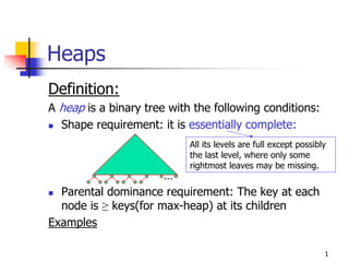
A heap is a binary tree with the following conditions:
Shape requirement: it is essentially complete:
All its levels are full except possibly
the last level, where only some
rightmost leaves may be missing.
…
Parental dominance requirement: The key at each
node is ≥ keys(for max-heap) at its children
Examples
1
2. Heaps and Heapsort
Not only is the heap structure useful for heapsort,
but it also makes an efficient priority queue.
Heapsort
In place
O(nlogn)
A priority queue is the ADT for maintaining a set S of
elements, each with an associated value called a
key/priority. It supports the following operations:
find element with highest priority
delete element with highest priority
insert element with assigned priority
2
3. Properties of Heaps (1)
Heap and its array representation. 9
Conceptually, we can think of a heap as
a binary tree. 5 3
But in practice, it is easier and more
efficient to implement a heap using an
array. 1 4 2
Store the BFS traversal of the heap’s
elements in position 1 through n, 1 2 3 4 5 6
leaving H[0] unused.
Relationships between indexes of 9 5 3 1 4 2
parents and children.
PARENT(i) LEFT(i) RIGHT(i)
return ⎣i/2⎦ return 2i return 2i+1
3
4. Properties of Heaps (2)
Max-heap property and min-heap property
Max-heap: for every node other than root, A[PARENT(i)] >= A(i)
Min-heap: for every node other than root, A[PARENT(i)] <= A(i)
The root has the largest key (for a max-heap)
The subtree rooted at any node of a heap is also a heap
Given a heap with n nodes, the height of the heap,
h = log n .
- Height of a node: the number of edges on the longest simple
downward path from the node to a leaf.
- Height of a tree: the height of its root.
- level of a node: A node’s level + its height = h, the tree’s height.
4
5. Bottom-up Heap construction
Build an essentially complete binary tree by inserting n
keys in the given order.
Heapify a series of trees
Starting with the last (rightmost) parental node, heapify/fix the
subtree rooted at it: if the parental dominance condition does
not hold for the key at this node:
1. exchange its key K with the key of its larger child
2. Heapify/fix the subtree rooted at it (now in the child’s position)
Proceed to do the same for the node’s immediate predecessor.
Stops after this is done for the tree’s root.
Example: 4 1 3 2 16 9 10 14 8 7 16 14 10 8 7 9 3 2 4 1
5
6. Bottom-up heap construction algorithm(A
Recursive version)
ALGORITHM HeapBottomUp(H[1..n])
//Constructs a heap from the elements Given a heap of n nodes, what’s
//of a given array by the bottom-up algorithm the index of the last parent?
//Input: An array H[1..n] of orderable items
//Output: A heap H[1..n] ⎣n/2⎦
for i ⎣n/2⎦ downto 1 do
MaxHeapify(H, i) ALGORITHM MaxHeapify(H, i)
l LEFT(i)
r RIGHT(i)
if l <= n and H[l] > H[i] // if left child exists and > H[i]
then largest l
else largest i
if r <= n and H[r] > H[largest] // if R child exists and > H[largest]
then largest r
if largest ≠ i
then exchange H[i] H[largest] // heapify the subtree
MaxHeapify(H, largest)
6
7. Bottom-up heap construction algorithm(An
Iterative version)
// from the last parent down to 1, heapify the subtree rooted at i
// k: the root of the subtree to be heapified; v: the key of the root
// if not a heap yet and the left child exists
// find the larger child, j: its index.
// if the key of the root > that of the larger child, done.
// exchange the key with the key of the larger child
// again, k: the root of the subtree to be heapified; v: the key of the root
7
8. Worst-Case Efficiency
Worst case:
a full tree; each key on a certain level will travel to the leaf.
Fix a subtree rooted at height j: 2j comparisons
Fix a subtree rooted at level i : 2(h-i) comparisons
A node’s level + its height = h, the tree’s height.
Total for heap construction phase:
h-1
Σ 2(h-i) 2
i=0
i = 2 ( n – lg (n + 1)) = Θ(n)
# nodes at level i
8
9. Bottom-up vs. Top-down Heap Construction
Bottom-up: Put everything in the array
and then heapify/fix the trees in a
bottom-up way.
Top-down: Heaps can be constructed
by successively inserting elements (see
the next slide) into an (initially) empty
heap.
9
10. Insertion of a New Element
The algorithm
Insert element at the last position in heap.
Compare with its parent, and exchange them if it violates the parental
dominance condition.
Continue comparing the new element with nodes up the tree until the
parental dominance condition is satisfied.
Example 1: add 10 to a heap: 9 6 8 2 5 7
Efficiency: h ∈ O(logn)
Inserting one new element to a heap with n-1 nodes requires no more
comparisons than the heap’s height
Example 2: Use the top-down method to build a heap for numbers 2 9 7 6 5 8
Questions
What is the efficiency for a top-down heap construction algorithm for a heap
of size n?
Which one is better, a bottom-up or a top-down heap construction?
10
11. Root Deletion
The root of a heap can be deleted and the heap
fixed up as follows:
1. Exchange the root with the last leaf
2. Decrease the heap’s size by 1
3. Heapify the smaller tree in exactly the same
way we did it in MaxHeapify().
It can’t make key comparison more
Efficiency: 2h ∈Θ(logn) than twice the heap’s height
Example: 9 8 6 2 5 1
11
12. Heapsort Algorithm
The algorithm
(Heap construction) Build heap for a given
array (either bottom-up or top-down)
(Maximum deletion ) Apply the root-
deletion operation n-1 times to the
remaining heap until heap contains just
one node.
An example: 2 9 7 6 5 8
12
13. Analysis of Heapsort
Recall algorithm:
Θ(n) 1. Bottom-up heap construction
Θ(log n) 2. Root deletion
Repeat 2 until heap contains just one node.
n – 1 times
Total: Θ(n) + Θ( n log n) = Θ(n log n)
• Note: this is the worst case. Average case also Θ(n log n).
13
14. Problem Reduction
Problem Reduction
If you need to solve a problem, reduce it to another problem that you
know how to solve.
Linear programming
A problem of optimizing a linear function of several variables subject to
constraints in the form of linear equations and linear inequalities.
Formally,
Maximize(or minimize) c1x1+ …Cnxn
Subject to ai1x1+…+ ainxn ≤ (or ≥ or =) bi, for i=1…n
x1 ≥ 0, …, xn ≥ 0
Reduction to graph problems
14
15. Linear Programming—Example 1:
Investment Problem
Scenario
A university endowment needs to invest $100million
Three types of investment:
Stocks (expected interest: 10%)
Bonds (expected interest: 7%)
Cash (expected interest: 3%)
Constraints
The investment in stocks is no more than 1/3 of the money
invested in bonds
At least 25% of the total amount invested in stocks and
bonds must be invested in cash
Objective:
An investment that maximizes the return
15
16. Example 1 (cont’)
Maximize 0.10x + 0.07y + 0.03z
subject to x + y + z = 100
x ≤(1/3)y
z ≥ 0.25(x + y)
x ≥ 0, y ≥ 0, z ≥ 0
16
17. Linear Programming—Example 2 :
Election Problem
Objective:
Scenario:
A politician that tries to win an Figure out the minimum
election. amount of money that you
Three types of areas of the district: need to spend in order to
win
urban (100,000 voters),
suburban (200,000 voters), and 50,000 urban votes
rural(50,000 voters). 100,000 suburban votes
Primary issues: 25,000 rural votes
Building more roads constraints:
Gun control
Policy Urban Suburban rural
Farm subsidies
Gasoline tax Build roads -2 5 3
Advertisement fee Gun control 8 2 -5
For every $1,000… Farm subsidies 0 0 10
Gasoline tax 10 0 -2 17
18. Example 2 (cont’)
x: the number of thousand of dollars spent on advertising on
building roads
y: the number of thousand of dollars spent on advertising on gun
control
z: the number of thousand of dollars spent on advertising on farm
subsidies
w: the number of thousand of dollars spent on advertising on
gasoline taxes
Maximize x + y + z + w
subject to –2x + 8y + 0z + 10w ≥ 50
5x + 2y + 0z + 0w ≥ 100
3x – 5y + 10z - 2w ≥ 25
x, y, z, w ≥ 0
18
19. Linear Programming—Example 3: Knapsack
Problem (Continuous/Fraction Version)
Scenario
Given n items:
weights: w1 w2 … wn
values: v1 v2 … vn
a knapsack of capacity W
Constraints
Any fraction of any item can be put into the knapsack.
All the items must fit into the knapsack.
Objective:
Find the most valuable subset of the items
19
20. Example 3 (cont’)
Maximize n
∑v x
j =1
j j
subject to n
∑w x
j =1
j j ≤W
0 ≤ xj ≤ 1 for j = 1,…, n.
20
21. Linear Programming—Example 3: Knapsack
Problem (Discrete Version)
Scenario
Given n items:
weights: w1 w2 … wn
values: v1 v2 … vn
a knapsack of capacity W
Constraints
an item can either be put into the knapsack in its entirely or
not be put into the knapsack.
All the items must fit into the knapsack.
Objective:
Find the most valuable subset of the items
21
22. Example 3 (cont’)
Maximize n
∑v x
j =1
j j
subject to n
∑w x
j =1
j j ≤W
xj ∈ {0,1} for j = 1,…, n.
22
23. Algorithms for Linear Programming
Simplex algorithm: exponential time.
Ellipsoid algorithm: polynomial time.
Interior-point methods: polynomial time.
Integer linear programming problem
no polynomial solution.
requires the variables to be integers.
23