matlab code cellular mobile communication

1. In this directory, we can find the eleven files. The relationship between file
name and the number of program written in the book is shown in as follows.
Program7-1 dcamain.m
Program7-2 basest.m
Program7-3 wrap.m
Program7-4 cellmesh.m
Program7-5 holdtime.m
Program7-6 shadow.m
Program7-7 dist.m
Program7-8 main.m
Program7-9 set_D.m
Program7-10 stationInit.m
Program7-11 antgain.m
If you would like to try to use the above programs by using MATLAB.
First of all, please copy all of files to your created adequate directory.
Then, you start to run MATLAB and you can see the following command prompt in
the command window.
>>
Next, you can go to the directory that have all of programs in this section by
using change directory (cd) commmand. If you copy all of files to
/matlabR12/work/chapter7, you only type the following command.
>>cd /matlabR12/work/chapter7
As for chapter7, we have two main functions: dcamain.m and main.m.
7.1 Simulation and evaluation procedure for dcmain.m
For the simulation dcmain.m, you just type the following command.
>>dcamain
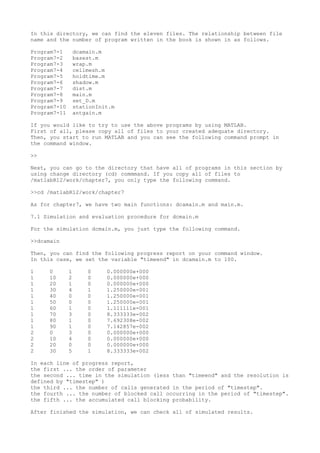
Then, you can find the following progress report on your command window.
In this case, we set the variable "timeend" in dcamain.m to 100.
1 0 1 0 0.000000e+000
1 10 2 0 0.000000e+000
1 20 1 0 0.000000e+000
1 30 4 1 1.250000e-001
1 40 0 0 1.250000e-001
1 50 0 0 1.250000e-001
1 60 1 0 1.111111e-001
1 70 3 0 8.333333e-002
1 80 1 0 7.692308e-002
1 90 1 0 7.142857e-002
2 0 3 0 0.000000e+000
2 10 4 0 0.000000e+000
2 20 0 0 0.000000e+000
2 30 5 1 8.333333e-002
In each line of progress report,
the first ... the order of parameter
the second ... time in the simulation (less than "timeend" and the resolution is
defined by "timestep" )
the third ... the number of calls generated in the period of "timestep".
the fourth ... the number of blocked call occurring in the period of "timestep".
the fifth ... the accumulated call blocking probability.
After finished the simulation, we can check all of simulated results.

2. (1) To see time transition of the accumulated blocking probability and the
forced termination probability
The time-transitions of the accumulated call blocking probability and the
accumulated forced termination probability during simulation period with the
time resolution of "timestep" are stored in the matrices, "check" and "check2"
respectively, changing the number of users per cell as a parameter. When we want
to see the time-transition of the accumulated call blocking probability as to
second parameter (the number of users), we have just to type the following
command.
>> plot(check(2, :))
(2) To see the results of the blocking probability and the forced termination
probability
After finishing simulation, the number of generation calls, the number of call
blocking, the call blocking probability, and the forced termination probability
will be stored in the matrix "output". Especially,
output(1,:)...the number of generated calls
output(2,:)...the number of blocked calls
output(3,:)...the call blocking probability
output(4,:)...the forced termination probability.
On the other hand, the number of users is given in the vector "usernum" (a
vector that gives parameters). When you would like to the relationship between
the number of users and the call blocking probability on the semilog graph, you
just type the following command.
>> semilogy(usernum, output(3, :))
If you would like to see the relationship between the number of generated calls
and the forced termination probability, you just type the following command.
>> semilogy(output(1, :), output(4, :))
(3) Save the results of blocking probability and forced termination probability
All of the simulation results for the call blocking probability and the forced
termination probability are stored to the file "data.txt" in the same directory
that stored the simulation programs.
7.2 Simulation and evaluation procedure for main.m
To simulate main.m, the following procedure must be needed.
(1) Set parameters
First of all, we set simulation parameters in "main.m".
(a) Characteristics of antenna gain decision for BS
(a-1) [horizontal]: beam width at BS for the target direction [degree]
w_HBS = 60;
(a-2) [horizontal]: antenna gain at BS for the opposite direction [dB]
backg_BS = -100;
(a-3) [vertical]: beam width at BS [degree]
w_VBS = 360;
(b) Characteristics of antenna gain decision for MS
(b-1) [horizontal]: beam width at MS for the target direction [degree]
w_HMS = 360;
(b-2) [horizontal]: antenna gain at MS for the opposite direction [dB]

3. backg_MS = -100;
(b-3) % [vertical]:beam width at MS [degree]
w_VMS = 360;
(2) Just type the following command
>> clear
>> main
(3) You can find a value that mentions the benefit provided by beamforming as
>> ans=
(4) When you change the valiable "w_HBS" from 30 to 80, you can find the same
value as shown in Fig. 7.20. To obtain the graph, you can change some points in
the program "main.m"
(a) Set alpha=3.5 and sigma=0
(b) For the following part in the program "main.m", you must remove the comment
command "%".
%-----Calculation of CIR under various w_HBS
% ii = 1;
% for w_HBS2=30:10:180,
% g_HBS2 = antgain(w_HBS2, backg_BS);
% CIdB_a2= Ptm_0(1:19)+g_HBS2(degHBS(1:19)+1) + g_VBS(degVBS(1:19)+1) +
g_HMS(degHMS(1:19)+1) + g_VMS(degVMS(1:19)+1)- Loss(2,1:19)-g(1:19); %
Received level at central BS (beam)
% CIw_a2 = 10 .^ ( CIdB_a2 ./ 10 ); % dB