Data science exercise to analyze A/B test results with moderator variables Instructions: https://raw.githubusercontent.com/benspaul/referer/gh-pages/Readme.txt Repo: https://github.com/benspaul/referer The image on the first page is stretched so that it will take up the entire thumbnail area on my LinkedIn profile.

2. A/B test with three-way ANOVA
Ben Paul
May 22, 2015
Background
• We tested two versions of a landing page in order to determine which had a greater return on investment
(ROI).
• We also collected data about tra c source (“referer”) and country of origin, to determine if the e ect
of landing page was di erent depending on the referer and country.
Hypotheses
• No hypotheses were specified.
Method
• Since no hypotheses were specified in advance, the data set was randomly split in half so that one half
could be used to generate hypotheses (the “exploratory” data set) and the other half could be used to
test those hypotheses (the “validation” data set).
• In particular, an ANOVA was conducted on the exploratory data set to assess the e ects of landing
page, country, and referer on ROI. E ects found in the exploratory data set were re-tested in the
validation set.
Analysis
Set up environment
1

3. library("plyr")
library("dplyr")
library("ggplot2")
library("lmtest")
source("interaction.t.tests.R")
knitr::opts_chunk$set(comment = NA) # remove hashes in output
knitr::opts_chunk$set(fig.width = 12) # increase plot width
theme_set(theme_gray(base_size = 12)) # decrease font size
Read data
dat <- read.csv("data/referer_data.csv")
Split data
set.seed(25)
samp <- sample(nrow(dat), nrow(dat) / 2)
explore <- dat[samp, ]
validate <- dat[-samp, ]
Clean data
Handle data types Check that data types are appropriate.
summary(explore, maxsum = 10); str(explore);
referer country landing_page roi
blogher : 1483 AU : 2457 a:24983 Min. : 5.63
caranddriver : 1479 CA : 9966 b:25017 1st Qu.: 15.43
FB :12573 Other: 2519 Median : 18.44
footballoutsider: 1542 UK :10002 Mean : 37.16
Google :24840 US :25056 3rd Qu.: 63.77
MSmag : 1462 Max. :182.76
Other : 1572
pioneeringwoman : 1499
scify : 1565
YouTube : 1985
data.frame : 50000 obs. of 4 variables:
$ referer : Factor w/ 10 levels "blogher","caranddriver",..: 9 3 5 3 5 5 3 10 1 5 ...
$ country : Factor w/ 5 levels "AU","CA","Other",..: 5 4 5 3 5 3 5 4 4 4 ...
$ landing_page: Factor w/ 2 levels "a","b": 1 1 2 2 1 1 2 2 1 2 ...
$ roi : num 39.49 44.61 15.43 8.65 15.43 ...
Data types appear to be appropriate. Referer, country, and landing_page are defined as factors, and roi is
numeric, as expected.
2

4. ROI ranges from 5.63 to 182.76. Assuming the unit is cents, these values would appear to be within reason for
a website visit. (It is di cult to find comparable benchmarks, but related data on average revenue per unique
visitor can be found at http://www.businessinsider.com/chart-of-the-day-revenue-per-unique-visitor-2011-1.
Since our data concern profit rather than revenue, it would make sense that our numbers are much lower
than those from the Business Insider article.)
Analyze data
Diagnostics A three-way ANOVA was planned to test the e ect of landing page, country, and referer on
ROI. Since we are analyzing a landing page test, only terms that included the landing page variable were
entered into the analysis: landing page, country x landing page, referer x landing page, and country x referer
x landing page.
Before inspecting the results, diagnostic plots were inspected to ensure ANOVA assumptions were met.
explore_fit <- aov(roi ~ landing_page + landing_page:referer + landing_page:country + landing_page:count
layout(1)
plot(explore_fit, 1)
0 50 100 150
−5e−090e+005e−09
Fitted values
Residuals
aov(roi ~ landing_page + landing_page:referer + landing_page:country + land ...
Residuals vs Fitted
69476
12439
98507
In this plot, the vast majority of the 500,000 residuals appear to have no relationship with fitted values.
However, it appears that heteroscedasticity may be present: there are about 10-20 data points with low fitted
values that seem to be associated with greater residual variation compared to those with higher fitted values.
But since it is di cult to tell from visual inspection if this represents significant heteroscedasticity, a formal
test for heteroscedasticity was run.
# Breusch-Pagan test for heteroscedasticity
bptest(explore_fit)
studentized Breusch-Pagan test
data: explore_fit
BP = 34.944, df = 99, p-value = 1
The test failed to detect heteroscedasticity, p = 1. Thus, heteroscedasticity is not a concern. The next
diagnostic was to check if nonnormality is present.
3

5. layout(1)
plot(explore_fit, 2)
−4 −2 0 2 4
−100050100150
Theoretical Quantiles
Standardizedresiduals
aov(roi ~ landing_page + landing_page:referer + landing_page:country + land ...
Normal Q−Q
69476
12439
98507
The data appear to be very nearly normal, although there are deviations in the tails that appear to a ect
about 20 of the 500,000 data points. Again, this is not thought to be a large enough concern to merit further
action. ANOVA assumptions appear to be reasonably met and we can proceed with analyzing the results.
explore_fit %>% drop1(.~., test = "F") # use Type III SS so that variable order doesn t matter - see htt
ANOVA
Warning: attempting model selection on an essentially perfect fit is
nonsense
Single term deletions
Model:
roi ~ landing_page + landing_page:referer + landing_page:country +
landing_page:country:referer
Df Sum of Sq RSS AIC F value
<none> 0 -2367527
landing_page 1 22272 22272 -40237 8.1789e+24
landing_page:referer 18 1120353 1120353 155633 2.2857e+25
landing_page:country 8 672600 672600 130140 3.0875e+25
landing_page:referer:country 72 0 0 -601608 1.5156e+18
Pr(>F)
<none>
landing_page < 2.2e-16 ***
landing_page:referer < 2.2e-16 ***
landing_page:country < 2.2e-16 ***
landing_page:referer:country < 2.2e-16 ***
---
Signif. codes: 0 *** 0.001 ** 0.01 * 0.05 . 0.1 1
The main e ect of landing page was significant, qualified by statistically significant interactions with referer
and with country (all ps < 0.001). Although the three-way interaction between landing page, referer, and
4

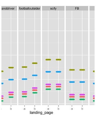
6. country was also statistically significant, it is associated with a sum of squares = 0, indicating that it did not
explain any variance. Therefore, it will not be interpreted.
To visualize the e ects, all data points were plotted, with landing page on the x-axis and ROI on the y-axis,
and graphs faceted by referer and colored by country. The order of referers was changed to demonstrate the
results more clearly.
# reorder referer levels
ref_levels <- c("blogher", "MSmag", "pioneeringwoman",
"caranddriver", "footballoutsider",
"scify", "FB", "Google", "YouTube", "Other")
explore <- within(explore, referer <- factor(referer, levels = ref_levels))
ggplot(explore, aes(x = landing_page, y = roi)) +
geom_jitter(alpha = 0.5, aes(color = country), position = position_jitter(width = 0.2, height = 0.1))
facet_wrap(~referer, nrow = 1)
blogher MSmag pioneeringwoman caranddriver footballoutsider scify FB Google YouTube Other
0
50
100
150
a b a b a b a b a b a b a b a b a b a b
landing_page
roi
country
AU
CA
Other
UK
US
The interaction between referer and landing page can be seen in that some referers have greater ROI with
landing page “a”, others have greater ROI with landing page “b”, and others have no di erence. Follow-up
t-tests were conducted to verify this e ect.
The interaction between country and landing page is not visible from the graph and may be of a much lower
magnitude. Follow-up t-tests were conducted to verify this e ect as well.
# set p-value cutoff using Bonferroni correction considering we are running several tests:
# (1) for each referer, run t-test comparing ROI from "a" vs. "b"
# (2) for each country, run t-test comparing ROI from "a" vs. "b"
p_cutoff <- 0.05 / (length(levels(explore$referer)) * 2)
# tests with referer
explore %>% interaction.t.tests(iv = "referer", group_var = "landing_page", dv = "roi", p_cutoff = p_cut
[1] " *** blogher: a had 31.74 greater roi, p = 0.00"
[1] " *** MSmag: a had 31.19 greater roi, p = 0.00"
[1] " *** pioneeringwoman: a had 30.57 greater roi, p = 0.00"
[1] " *** caranddriver: b had 6.95 greater roi, p = 0.00"
[1] " *** footballoutsider: b had 7.56 greater roi, p = 0.00"
[1] "scify: no difference in roi, p = 0.93"
5

7. [1] "FB: no difference in roi, p = 0.69"
[1] "Google: no difference in roi, p = 0.14"
[1] "YouTube: no difference in roi, p = 0.58"
[1] "Other: no difference in roi, p = 0.93"
# tests with country
explore %>% interaction.t.tests(iv = "country", group_var = "landing_page", dv = "roi", p_cutoff = p_cut
[1] " *** AU: a had 2.33 greater roi, p = 0.00"
[1] " *** CA: a had 2.35 greater roi, p = 0.00"
[1] " *** Other: a had 1.69 greater roi, p = 0.00"
[1] " *** UK: a had 2.36 greater roi, p = 0.00"
[1] " *** US: a had 1.90 greater roi, p = 0.00"
Results indicate that:
• Landing page “a” had greater ROI than landing page “b” for referers “blogher”, “MSmag”, and
“pioneeringwoman” (p < 0.001, ROI di erences range from 31 - 32).
• Landing page “b” had greater ROI than landing page “a” for referers “caranddriver” and “footballout-
sider”" (p < 0.001, ROI di erences range from 7 - 8).
• Landing pages “a” and “b” did not have di erent ROIs for referers “scify”, “FB”, “Google”, “YouTube”,
and “Other” (all ps > 0.1).
• Landing page “a” ROI is greater than “b” by two units (presumably cents) regardless of country; despite
the statistically significant interaction e ect between the two variables, the t-test results above show
that the e ect of landing page di ers by less than one cent from country to country (ROI di erences
range from 1.69 - 2.36 cents). Since the magnitude of this e ect is extremely low compared to other
e ects seen in the data, it is considered to be of minimal importance and will not be interpreted further.
The referer by landing page interaction was re-tested in the validation data set.
# reorder referer levels
ref_levels <- c("blogher", "MSmag", "pioneeringwoman",
"caranddriver", "footballoutsider",
"scify", "FB", "Google", "YouTube", "Other")
validate <- within(validate, referer <- factor(referer, levels = ref_levels))
validate %>% interaction.t.tests(iv = "referer", group_var = "landing_page", dv = "roi")
[1] " *** blogher: a had 31.74 greater roi, p = 0.00"
[1] " *** MSmag: a had 31.19 greater roi, p = 0.00"
[1] " *** pioneeringwoman: a had 30.57 greater roi, p = 0.00"
[1] " *** caranddriver: b had 6.95 greater roi, p = 0.00"
[1] " *** footballoutsider: b had 7.56 greater roi, p = 0.00"
[1] "scify: no difference in roi, p = 0.93"
[1] "FB: no difference in roi, p = 0.69"
[1] "Google: no difference in roi, p = 0.14"
[1] "YouTube: no difference in roi, p = 0.58"
[1] "Other: no difference in roi, p = 0.93"
The same results are seen (all ps < 0.001), so the hypotheses have been supported. Just as in the exploratory
set:
6

8. • Landing page “a” had greater ROI than landing page “b” for referers “blogher”, “MSmag”, and
“pioneeringwoman” (p < 0.001, ROI di erences range from 31 - 32, same as exploratory results).
• Landing page “b” had greater ROI than landing page “a” for referers “caranddriver” and “footballout-
sider”" (p < 0.001, ROI di erences range from 7 - 8, same as exploratory results).
• Landing pages “a” and “b” did not have di erent ROIs for referers “scify”, “FB”, “Google”, “YouTube”,
and “Other” (all ps > 0.1, same as exploratory results).
Discussion
The referers whose tra c benefits from landing page “a” all appear to be targeted at females (blogher,
MSmag, pioneeringwoman). Assuming that these referers are associated with blogher.com, msmagazine.com,
and thepioneerwoman.com, data from Alexa confirm that females are “greatly over-represented” in their
tra c (http://www.alexa.com/siteinfo/blogher.com, http://www.alexa.com/siteinfo/msmagazine.com, http:
//www.alexa.com/siteinfo/thepioneerwoman.com).
In contrast, referers whose tra c benefits from page “b” appear to be targeted at males (caranddriver,
footballoutsider). Assuming that these referers are associated with caranddriver.com and footballout-
siders.com, data from Alexa confirm that males are “over-represented” in the former (http://www.alexa.
com/siteinfo/caranddriver.com) and “greatly over-represented” in the latter (http://www.alexa.com/siteinfo/
footballoutsiders.com).
Finally, referers whose tra c benefits equally from page “a” and “b” appear to be targeted at both males
and females roughly equally. Although Alexa data are not available for “scify”, Quantcast data for syfy.com
(which used to be scify.com) shows the genders are roughly even, with only slightly more males (https:
//www.quantcast.com/syfy.com). Alexa data for youtube.com, facebook.com, and google.com also show a
similar pattern: there are some gender di erences but not nearly to the magnitude of that seen in sites like
caranddriver.com and msmagazine.com.
In light of this finding, it may be worthwhile to assign all tra c from overwhelmingly female referers to see
landing page “a” and all tra c from overwhelmingly male referers to see landing page “b”. We would monitor
overall ROI to ensure that it increases after this change.
In addition, it may be worthwhile to conduct user interviews to try to discern why the pages appeal to
di erent genders. For example, it could be found that the title at the top of landing page “a” resonates with
females, while an image on the page does not. Di erent versions of the image more aligned with the message
could then be attempted in an e ort to further increase ROI.
7