Custom Duties in India. Term paper (2007) MSE

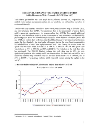
1. INDIAN PUBLIC FINANCE TERMPAPER: CUSTOMS DUTIES
Ashish Bharadwaj, M.Sc. Economics II, MSE (Nov 2007)
The central government has four major taxes: personal income tax, corporation tax,
central excise duties and customs duties. In our analysis, we will confine ourselves to
customs duties only.
The customs duty in India consists of ‘basic’ tariff, the additional duty of customs (AD),
and special excise duty (SAD). The additional duty is the counterpart of excise duties
paid by domestic manufacturers i.e. countervailing duty (CVD). The special additional
duty has been introduced to serve as the counterpart of state sales taxes on domestically
produced goods. Since the customs duty is collected under the three sub-heads (basic, AD
and SAD), its custom duty collection rate should be obtained by dividing total collections
under the three heads by the total value of imports during the year. Some commodities
like alcohol have a ‘basic’ rate higher than the ‘peak’ rate. During the reform years, the
“peak” rate has come down from 150 % in 1991-92 to 40 % in 1997-98. The “peak” rate
was reduced to 35% in 2001-02 and 30% in 2002-03. The reduction in the peak duty rates
has continued. The 2005-06 Budget reduced the peak duty rate to 15% for nonagricultural products. The average tariff rate has therefore declined over the 1990s. As a
result the customs duty collection rate has declined from about 47% in 1998-99, and to
21% in 2000-01. The average customs tariffs rates still remain among the highest in the
world 1 .
1. Revenue Performance of Customs and Excise Duty relative to GDP
Excise and Customs revenue as % of GDP
6.00
Revenue (as % GDP)
5.00
4.00
3.00
2.00
1.00
2002-03
2000-01
1998-99
1996-97
1994-95
1992-93
1990-91
1988-89
1986-87
1984-85
1982-83
1980-81
1978-79
1976-77
1974-75
1972-73
1970-71
1968-69
1966-67
1964-65
1962-63
1960-61
1958-59
1956-57
1954-55
1952-53
1950-51
0.00
Year
Excise revenue as % of GDP
1
Customs revenue as % of GDP
Srivastava, D.K., “Issues in Indian Public Finance”(2005), New Delhi
1

2. The profile of the share of the customs duties shows more of an inverted U-shape, similar
to Union excise duties, although these started at a level much higher than excise duties. In
1950-51, the customs duties accounted for nearly 1.6% of GDP, which was the highest
among all major central taxes. (Table 1, Appendix A) These were overtaken by excise
duties in 1957-58. Following a slightly volatile pattern, these reached a peak of 3.9% in
1986-87, after which they started declining. By 2001-02, these had reached a level,
relative to GDP, of 1.8%, which is compared to its level in the mid sixties. Thus, customs
duty, which was the highest contributor, is fast becoming the lowest contributor now.
2. Relative Shares of Major Central Taxes in Centre's Gross Tax Revenues
60.0
50.0
Share in %
40.0
30.0
20.0
10.0
2002-03
2000-01
1998-99
1996-97
1994-95
1992-93
1990-91
1988-89
1986-87
1984-85
1982-83
1980-81
1978-79
1976-77
1974-75
1972-73
1970-71
1968-69
1966-67
1964-65
1962-63
1960-61
1958-59
1956-57
1954-55
1952-53
1950-51
0.0
Year
Income Tax
Corporation Tax
Excise Duty
Customs Duty
The chart highlights the inverted U-shape of the curve representing the share of Union
excise duties, which can be contrasted with the more U-shape type of curve of the
customs duties until the beginning of the nineties. What is also clearly observable is that
the four taxes are tending to come close to each other in terms of their shares in the
centre’s gross revenue receipts. (Table 2, Appendix A)
3. Customs Duties: Annual Buoyancy
Tax buoyancy is measured as % change in tax revenue over a given period by % change
in tax base, which is generally taken to be GDP, over the same period.
While the contribution that a tax makes to overall collection of tax revenues is an
important consideration, another important feature of the tax sources is their volatility. To
examine this, we look at the yearly growth rates. Customs duties are more noticeable for
their negative growth in more recent years. (Table 3, Appendix A)
2

3. Annual Customs Duty Buoyancy
15.00
10.00
Buoyancy
5.00
2001-02
1999-00
1997-98
1995-96
1993-94
1991-92
1989-90
1987-88
1985-86
1983-84
1981-82
1979-80
1977-78
1975-76
1973-74
1971-72
1969-70
1967-68
1965-66
1963-64
1961-62
1959-60
1957-58
1955-56
1953-54
1951-52
0.00
-5.00
-10.00
Year
Comparison of custom rate among countries
16.8
China
22.2
Bangladesh
20
Sri Lanka
7.1
Malaysia
S.Korea
8.7
Taiwan
8.8
10.9
Country
Indonesia
17.1
Thailand
20.5
Egypt
13.9
Russia
11
Argentina
10.1
Mexico
10
Chile
8.5
S.Africa
8.2
Turkey
32.2
India
0
5
10
15
20
25
30
35
Custom Tariff Rate
3

4. EMPIRICAL STUDY I
Testing for Cointegration between the following
a) Customs Revenues and Other Central Tax Revenues such as Personal
Income Tax, Corporation Tax and Total Direct Tax Revenues (1970-2006)
b) Customs Revenues and Imports of Principal Commodities 2
Dependent Variable:
CR = customs revenues {Yt}
Possible Independent Variables {Xt} to test for Cointegration with CR
ER = excise revenues
ITR = income tax revenues
CTR = corporation tax revenues
DTR = total direct tax revenues
IMP = imports
Yt = β0 + β1Xt + ut
Yt, Xt ~ Cointegration (d,b) if both series are integrated of same order i.e. d=b
Testing for Stationary using Augmented Dickey-Fuller Test (ADF Test)
Variable
First Difference
ADF Test Statistics*
Second Difference
Δ CRt
-3.05
(stationary)
-
ERt
ADF Test
Statistics*
0.837
(non
stationary)
3.818
Δ ERt
Δ ERt-1
ITRt
3.710
Δ ITRt
CTRt
3.801
Δ CTRt
-0.958
(non stationary)
0.038
(non stationary)
0.907
(non stationary)
DTRt
4.319
Δ DTRt
IMPt
2.344
Δ IMPt
CRt
2.734
(non stationary)
3.514
(non stationary)
Δ ITRt-1
Δ CTRt-1
Δ DTRt-1
Δ IMPt-1
ADF Test
Statistics*
-
Order of
Integration
I(1)
-6.367
(stationary)
-4.256
(stationary)
-1.787
(non
stationary)
-3.104
(stationary)
-0.560
(non
stationary)
I(2)
*Compared with (-2.975) Critical Value at 5% level
(Table 4, Appendix B and Table 5, Appendix C)
Conclusion:
We can conclude that any regression model containing CR with any other variable
mentioned above would be meaningless and cannot be tested for Cointegration since
they are integrated of different orders.
2
Food & live animals, beverages & tobacco, Crude materials, inedible, except fuels, Mineral fuels, lubricants and
related materials, Animal and vegetable oils and fats, Chemicals, Manufacture goods classified chiefly by material,
Machinery and transport equipment, Miscellaneous manufactured articles
4
I(2)
> I(2)
I(2)
> I(2)

5. EMPIRICAL STUDY II
Testing for Causality between Customs Revenue and Effective Customs Duty
CR = Customs Revenue
ETR = Total Customs Revenue/GDPmp
Where ETR is the effective tax rate (customs duty) and GDP has been taken as a proxy
for a tax base for customs duty.
Ln CRt = β0 + β1 (ln ETRt) + β2 (lnETRt)2 + ut
Variable
ADF Test
First Difference
Statistics*
Ln CRt
-1.712
Δ ln CRt
(non stationary)
Ln ETRt
2.001
Δ ln ETRt
(non stationary)
(LnETRt)2
0.075
Δ ln ETR2t
(non stationary)
*Compared with (-2.975) Critical Value at 5% level
ADF Test
Statistics*
-3.611
(stationary)
-3.359
(stationary
-3.222
(stationary
Order of
Integration
I(1)
I(1)
I(1)
Ln CRt = 18.53 + 2.81(lnETRt) + 0.14(lnETRt)2
(4.91)
(2.28)
(14.49)
R2 = 0.9673
DW statistic = 0.13
Figures in parentheses are t-values (5% level of significance)
(Table 4, Appendix B and Table 5, Appendix C)
Testing for stationarity of residuals in the model using ADF test
ADF test statistic = -1.342
Interpolated DF 5% critical value = -2.972
MacKinnon approximate p-value = 0.6098
Observations:
1. Errors are non stationary
2. Durbin-Watson statistic value considerably less than 2.0 implies that the errors
serially correlated
Conclusion:
It can be concluded that the above regression is spurious since both X and Y variables are
stationary of same order but the error term is non-stationary. However, we can apply OLS
to the appropriately differenced series (taking into account the appropriate lag length
using either AIC or SC).
5

6. ΔlnCRt = 0.06 - 0.23ΔlnCRt-1 + 0.29ΔlnETRt-1 + 1.36ΔlnETRt + 0.04Δ (lnETRt) 2 + 0.007Δ (lnETRt-1)2
(5.9)
(-1.24)
(0.97)
(8.8)
(2.6)
(0.38)
ΔlnCRt = 0.057 - 0.11ΔlnCRt-1 + 0.09ΔlnETRt-1 + 0.95ΔlnETRt
(5.4) (-0.63)
(0.59)
(25.29)
ΔlnCRt = 0.03 + 0.26ΔlnCRt-1 – 0.1Δ (lnETRt) 2 + 0.03Δ (lnETRt-1)2
(2.93) (1.69)
(-13.5)
(1.92)
lnETR and (lnETR)2 Granger cause lnCR
EMPIRICAL STUDY III
Estimating a Laffer curve for customs duty revenues and effective rate (customs
duty) for India (1970-2006) using a log-lin model.
lnCRt = 228.8ETRt – 3012.2 (ETRt)2
(14.5)
(-7.6)
∂lnCR t
= 228.8 − 6024.4 ETRt
∂ETRt
∂lnCR t
= 0 => ETRt = 0.0379 or 3.79%
FOC:
∂ETRt
SOC:
R2 = 0.928
∂ 2 lnCR t
= −(6024.4) < 0
∂ETRt 2
Since the quadratic term is negative and significant, the Laffer curve has a bell shape. Taking the first
derivative of lnCR, with respect to ETR, and setting the first derivative to zero, we find that the
revenue-maximizing tax rate is 3.79%. This can also be seen from the graph below. We may draw a
conclusion that the Federal government is likely to raise more tax revenues by raising the tax rate up
to this level.
(Table 4, Appendix B and Table 5, Appendix C)
6

7. Appendix A
Table 1: Tax revenues as % of GDP (1950-51 to 2002-03)
Year
Excise
customs
Year
1950-51
0.68
1.58
1968-69
1951-52
0.81
2.21
1969-70
1952-53
0.80
1.68
1970-71
1953-54
0.48
1.41
1971-72
1954-55
1.01
1.73
1972-73
1955-56
1.34
1.55
1973-74
1956-57
1.47
1.34
1974-75
1957-58
2.05
1.35
1975-76
1958-59
2.10
0.93
1976-77
1959-60
2.30
1.00
1977-78
1960-61
2.43
0.99
1978-79
1961-62
2.69
1.17
1979-80
1980-81
1962-63
3.06
1.26
1981-82
1963-64
3.25
1.49
1982-83
1964-65
3.06
1.52
1983-84
1965-66
3.25
1.95
1984-85
1966-67
3.30
1.87
1985-86
1967-68
3.13
1.40
Source: Indian Public finance statistics, 2006
Excise
3.40
3.57
3.85
4.21
4.31
3.97
4.17
4.02
4.70
4.38
4.87
4.97
4.52
4.40
4.28
4.66
4.54
4.66
customs
1.15
0.99
1.15
1.42
1.59
1.52
1.72
1.71
1.73
1.80
2.20
2.42
2.37
2.55
2.72
2.54
2.87
3.43
Year
1986-87
1987-88
1988-89
1989-90
1990-91
1991-92
1992-93
1993-94
1994-95
1995-96
1996-97
1997-98
1998-99
1999-00
2000-01
2001-02
2002-03
Excise
4.65
4.64
4.47
4.61
4.31
4.30
4.12
3.69
3.69
3.38
3.29
3.15
3.06
3.20
3.28
3.19
3.34
customs
3.69
3.87
3.75
3.71
3.63
3.41
3.18
2.58
2.65
3.01
3.13
2.64
2.34
2.50
2.28
1.77
1.82
Table 2: Relative Share (in %) of Central Taxes in Gross Central Taxes
Year
1950-51
1951-52
1952-53
1953-54
1954-55
1955-56
1956-57
1957-58
1958-59
1959-60
1960-61
1961-62
1962-63
1963-64
1964-65
1965-66
1966-67
Income
33.0
28.6
27.6
29.1
28.9
27.2
26.5
23.8
24.5
16.9
18.9
15.7
14.5
15.5
14.6
13.2
13.4
Corp.tax
9.7
8.0
9.3
8.9
8.1
7.5
8.8
8.0
7.7
12.1
12.3
14.8
17.2
16.8
17.2
14.8
14.3
Excise
16.7
16.7
18.7
12.9
23.8
29.9
33.4
39.6
44.6
41.1
46.5
46.4
46.6
44.6
44.0
43.6
44.8
Customs
38.8
45.5
39.0
37.8
40.6
34.8
30.4
26.0
19.7
17.8
19.0
20.1
19.1
20.5
21.8
26.2
25.4
Year
1977-78
1978-79
1979-80
1980-81
1981-82
1982-83
1983-84
1984-85
1985-86
1986-87
1987-88
1988-89
1989-90
1990-91
1991-92
1992-93
1993-94
Income
11.3
11.2
11.2
11.4
9.3
8.9
8.2
8.2
8.8
8.8
8.5
9.6
9.8
9.3
10.0
10.6
12.0
Corp.tax
13.8
11.9
11.6
9.9
12.4
12.3
12.0
10.9
10.0
9.6
9.1
9.9
9.2
9.3
11.7
11.9
13.3
Excise
50.2
51.0
50.2
49.3
46.8
45.5
49.3
47.5
45.2
44.1
43.6
42.4
43.4
42.6
41.7
41.3
41.8
Customs
20.6
23.0
24.4
25.9
27.1
28.9
26.9
30.0
33.2
34.9
36.4
35.5
34.9
35.9
33.0
31.9
29.3
7

8. Contd
1967-68
1968-69
1969-70
1970-71
1971-72
1972-73
1973-74
1974-75
1975-76
1976-77
13.8
15.1
15.9
14.8
13.9
13.9
14.6
13.8
16.0
14.5
13.2
11.9
12.5
11.6
12.2
12.4
11.5
11.2
11.3
11.9
48.8
52.6
54.0
54.9
53.2
51.6
51.3
51.1
44.0
51.1
21.8
17.8
15.0
16.3
18.0
19.0
19.7
21.1
18.7
18.8
1994-95
1995-96
1996-97
1997-98
1998-99
1999-00
2000-01
2001-02
2002-03
13.0
14.0
14.1
12.3
14.1
14.9
16.8
17.1
16.6
15.0
14.8
14.3
14.4
17.1
17.9
18.9
19.6
20.8
40.5
36.1
34.7
34.4
37.0
36.0
36.3
38.8
37.1
29.0
32.2
33.0
28.9
28.3
28.2
25.2
21.5
20.2
Source: Indian Public finance statistics, 2006
Table 3: Estimated Annual Buoyancy of Central Taxes
Year
Income
Corp.tax
Excise
Customs
1951-52
1.52
0.57
4.23
7.58
1952-53
8.59
-1.02
1.65
13.43
1953-54
-0.05
-1.15
1.63
-0.98
1954-55
-1.39
0.15
-2.61
-3.08
1955-56
0.28
-0.77
18.74
-5.38
1956-57
0.76
1.99
0.63
0.21
1957-58
2.89
3.40
14.24
1.27
1958-59
0.39
-0.21
1.25
-2.03
1959-60
-2.50
17.85
2.83
2.39
1960-61
1.40
0.31
1.62
0.94
1961-62
-0.33
7.11
2.92
4.14
1962-63
1.65
5.52
2.96
2.11
1963-64
2.44
1.61
1.47
2.42
1964-65
0.31
0.86
0.59
1.13
1965-66
0.36
-0.53
2.18
6.45
1966-67
1.03
0.60
1.15
0.66
1967-68
0.33
-0.33
0.65
-0.72
1968-69
2.72
-0.58
2.53
-2.20
1969-70
1.83
1.77
1.52
-0.51
1970-71
0.81
0.71
2.24
3.48
1971-72
1.89
3.85
2.41
4.60
1972-73
1.61
1.77
1.25
2.26
1973-74
0.86
0.21
0.55
0.76
1974-75
0.99
1.20
1.34
1.87
1975-76
5.20
2.87
0.47
0.87
1976-77
-0.21
1.83
3.37
1.22
Source: Indian Public finance statistics, 2006
Year
1977-78
1978-79
1979-80
1980-81
1981-82
1982-83
1983-84
1984-85
1985-86
1986-87
1987-88
1988-89
1989-90
1990-91
1991-92
1992-93
1993-94
1994-95
1995-96
1996-97
1997-98
1998-99
1999-00
2000-01
2001-02
2002-03
Income
-1.22
2.08
1.42
0.65
-0.12
0.55
0.50
1.14
2.28
1.23
0.79
1.80
1.21
0.35
1.70
1.19
1.05
1.78
1.71
1.12
-0.55
1.28
2.38
3.02
0.09
1.80
Corp.tax
1.82
0.30
1.15
-0.31
2.91
0.93
0.85
0.21
0.91
0.86
0.62
1.50
0.48
0.76
3.18
0.91
0.88
2.09
1.11
0.83
0.69
1.57
2.23
2.07
0.29
3.10
Excise
0.41
2.46
1.23
0.43
0.82
0.74
1.62
0.77
1.22
0.98
0.97
0.78
1.24
0.55
0.99
0.66
0.19
1.00
0.44
0.79
0.58
0.77
1.45
1.36
0.67
1.60
Customs
1.32
3.91
2.13
0.88
1.51
1.63
0.55
2.20
2.67
1.71
1.40
0.81
0.92
0.85
0.53
0.47
-0.45
1.16
1.94
1.31
-0.55
0.08
1.69
-0.23
-1.75
1.35
8

9. Appendix B
Table 4: GDP & Import figures along with the calculated ETR (=Revenues/GDP)
Year
GDP at market prices
( at 1993-94 prices)
(in Rs.crore)
Imports
(in Rs.crore)
1970-71
326925
1634.2
1971-72
332516
1824.5
1972-73
330594
1867.4
1973-74
341050
2955.4
1974-75
345101
4518.8
1975-76
376731
5264.8
1976-77
383163
5073.8
1977-78
410873
6020.2
1978-79
434437
6810.6
1979-80
411663
9142.6
1980-81
439201
12549.2
1981-82
467139
13607.6
1982-83
484217
14292.7
1983-84
518491
15831.5
1984-85
539874
17134.2
1985-86
570267
19657.7
1986-87
597850
20095.8
1987-88
623371
22243.7
1988-89
684832
28235.2
1989-90
728952
35328.4
1990-91
771295
43192.9
1991-92
778289
47850.8
1992-93
819318
63374.5
1993-94
859220
73101.0
1994-95
923349
89970.7
1995-96
993946
122678.1
1996-97
1067444
138919.7
1997-98
1115248
154176.3
1998-99
1182020
178331.9
1999-00
1266283
215236.5
2000-01
1316201
230872.8
2001-02
1383705
245199.7
2002-03
1440632
297205.9
2003-04
1564620
359107.7
2004-05
1612201
501064.5
2005-06
1699056
660408.9
2006-07
1760539
862301.5
Source: CSO and Statistics on Indian Economy, RBI
Effective tax rate
(customs)
etr^2
0.001602814
0.002090125
0.002592304
0.002920393
0.003862637
0.003766613
0.004055715
0.004439328
0.005579635
0.007102897
0.007761822
0.009204969
0.010571706
0.010767786
0.013041932
0.016704456
0.019193778
0.02198049
0.023078653
0.02474237
0.026765375
0.028597346
0.029019257
0.02582924
0.029012865
0.035974791
0.040143558
0.036039518
0.034405509
0.038237108
0.025955762
0.020481244
0.022141671
0.022105048
0.025934111
0.02745348
0.033110315
0.000003
0.000004
0.000007
0.000009
0.000015
0.000014
0.000016
0.000020
0.000031
0.000050
0.000060
0.000085
0.000112
0.000116
0.000170
0.000279
0.000368
0.000483
0.000533
0.000612
0.000716
0.000818
0.000842
0.000667
0.000842
0.001294
0.001612
0.001299
0.001184
0.001462
0.000674
0.000419
0.000490
0.000489
0.000673
0.000754
0.001096
9

10. Appendix C
Table 5: Central Government Receipts of major components (Rs.crore)
Year
Indirect tax (net)
1970-71
1971-72
1972-73
1973-74
1974-75
1975-76
1976-77
1977-78
1978-79
1979-80
1980-81
1981-82
1982-83
1983-84
1984-85
1985-86
1986-87
1987-88
1988-89
1989-90
1990-91
1991-92
1992-93
1993-94
1994-95
1995-96
1996-97
1997-98
1998-99
1999-00
2000-01
2001-02
2002-03
2003-04
2004-05
2005-06
2006-07
Source: CSO and RBI
1940
2342
2691
3052
3956
4530
4895
5319
6726
6617
7465
9024
10294
12310
14276
17442
20296
23915
27730
32321
36075
39966
41969
40927
49045
59652
68326
68500
72532
86836
87007
85828
96932
110392
128854
149572
177201
Excise duties
(net)
1369
1586
1757
1971
2528
2988
3193
3335
4128
3481
3723
4181
4567
6165
6625
7331
8164
9423
10922
13096
14100
16017
16367
17224
21064
22176
23463
25516
28581
34944
49758
54469
62388
70245
77241
86642
92304
Customs
duties
524
695
857
996
1333
1419
1554
1824
2424
2924
3409
4300
5119
5583
7041
9526
11475
13702
15805
18036
20644
22257
23776
22193
26789
35757
42851
40193
40668
48419
34163
28340
31898
34586
41811
46645
58292
Income
tax
114
75
137
213
362
480
542
327
471
475
438
459
438
527
697
665
719
603
1492
1088
1250
1627
1831
1355
3468
4318
4715
3589
5760
9131
23766
22106
27779
30765
35443
45238
59667
Corporation
tax
371
472
558
583
709
862
984
1221
1256
1392
1311
1970
2185
2493
2556
2865
3160
3433
4407
4729
5335
7853
8899
10060
13822
16487
18567
20016
24529
30692
25177
25133
33893
45706
60289
75187
108880
10