topic models

1. Online Inference of Topics with Latent Dirichlet Allocation
Kevin R. Canini Lei Shi Thomas L. Griffiths
Computer Science Division Helen Wills Neuroscience Institute Department of Psychology
University of California University of California University of California
Berkeley, CA 94720 Berkeley, CA 94720 Berkeley, CA 94720
kevin@cs.berkeley.edu lshi@berkeley.edu tom griffiths@berkeley.edu
Abstract arrive in a continuous stream, and decisions must be
made on a regular basis, without waiting for future
documents to arrive. In these settings, repeatedly run-
Inference algorithms for topic models are typ-
ning a batch algorithm can be infeasible or wasteful.
ically designed to be run over an entire col-
lection of documents after they have been In this paper, we explore the possibility of using online
observed. However, in many applications of inference algorithms for topic models, whereby the rep-
these models, the collection grows over time, resentation of the topics in a collection of documents
making it infeasible to run batch algorithms is incrementally updated as each document is added.
repeatedly. This problem can be addressed In addition to providing a solution to the problem of
by using online algorithms, which update es- growing document collections, online algorithms also
timates of the topics as each document is open up different routes for parallelization of infer-
observed. We introduce two related Rao- ence from batch algorithms, providing ways to draw
Blackwellized online inference algorithms for on the enhanced computing power of multiprocessor
the latent Dirichlet allocation (LDA) model – systems, and different tradeoffs in runtime and perfor-
incremental Gibbs samplers and particle fil- mance from other algorithms.
ters – and compare their runtime and perfor-
We discuss algorithms for a particular topic model: la-
mance to that of existing algorithms.
tent Dirichlet allocation (LDA) (Blei et al., 2003). The
state space from which these algorithms draw samples
is defined at time i to be all possible topic assignments
1 INTRODUCTION to each of the words in the documents observed up to
time i. The result is a Rao-Blackwellized sampling
Probabilistic topic models are often used to analyze scheme (Doucet et al., 2000), analytically integrating
collections of documents, each of which is represented out the distributions over words associated with topics
as a mixture of topics, where each topic is a proba- and the per-document weights of those topics.
bility distribution over words. Applying these mod-
els to a document collection involves estimating the The plan of the paper is as follows. Section 2 intro-
topic distributions and the weight each topic receives duces the LDA model in more detail. Section 3 dis-
in each document. A number of algorithms exist for cusses one batch and three online algorithms for sam-
solving this problem (e.g., Hofmann, 1999; Blei et al., pling from LDA. Section 4 discusses the efficient im-
2003; Minka and Lafferty, 2002; Griffiths and Steyvers, plementation of one of the online algorithms – particle
2004), most of which are intended to be run in “batch” filters. Section 5 describes a comparative evaluation
mode, being applied to all the documents once they are of the algorithms, and Section 6 concludes the paper.
collected. However, many applications of topic mod-
els are in contexts where the collection of documents
is growing. For example, when inferring the topics
2 INFERRING TOPICS
of news articles or communications logs, documents
Latent Dirichlet allocation (Blei et al., 2003) is widely
Appearing in Proceedings of the 12th International Confe- used for identifying the topics in a set of documents,
rence on Artificial Intelligence and Statistics (AISTATS) building on previous work by Hofmann (1999). In this
2009, Clearwater Beach, Florida, USA. Volume 5 of JMLR: model, each document is represented as a mixture of
W&CP 5. Copyright 2009 by the authors.
a fixed number of topics, with topic z receiving weight
65

2. Online Inference of Topics with Latent Dirichlet Allocation
(d)
θz in document d, and each topic is a probability dis- Algorithm 1 batch Gibbs sampler for LDA
tribution over a finite vocabulary of words, with word 1: initialize zN randomly from {1, . . . , T }N
(z)
w having probability φw in topic z. The generative 2: loop
model assumes that documents are produced by inde- 3: choose j from {1, . . . , N }
pendently sampling a topic z for each word from θ(d) 4: sample zj from P (zj |zN j , wN )
and then independently sampling the word from φ(z) .
The independence assumptions mean that the docu-
ment is treated as a bag of words, so word ordering 3.1 BATCH GIBBS SAMPLER
is irrelevant to the model. Symmetric Dirichlet priors
are placed on θ(d) and φ(z) , with θ(d) ∼ Dirichlet(α) Griffiths and Steyvers (2004) presented a collapsed
and φ(z) ∼ Dirichlet(β), where α and β are hyper- Gibbs sampler for LDA, where the state space is the set
parameters that affect the relative sparsity of these of all possible topic assignments to the words in every
distributions. The complete probability model is thus document. The Gibbs sampler is “collapsed” because
the variables θ and φ are analytically integrated out,
wi |zi , φ(zi ) ∼ Discrete(φ(zi ) ), i = 1, . . . , N,
and only the latent topic variables zN are sampled.
φ(z) ∼ Dirichlet(β), z = 1, . . . , T,
The topic assignment of word j is sampled according
zi |θ(di ) ∼ Discrete(θ(di ) ), i = 1, . . . , N,
to its conditional distribution
θ(d) ∼ Dirichlet(α), d = 1, . . . , D,
(w ) (d )
where N is the total number of words in the collection, nzj ,N j + β nzj j j + α
j
,N
P (zj |zN j , wN ) ∝ , (1)
T is the number of topics, D is the number of docu- (·) (d )
j
nzj ,N j + W β n·,N j + T α
ments, and di and zi are, respectively, the document
and topic of the ith word, wi . The goal of inference in where zN j indicates (z1 , . . . , zj−1 , zj+1 , . . . , zN ), W is
this model is to identify the values of φ and θ, given a j (w )
the size of the vocabulary, nzj ,N j is the number of
document collection represented by the sequence of N
(·)
words wN = (w1 , . . . , wN ). Estimation is complicated times word wj is assigned to topic zj , nzj ,N j is the
by the latent variables zN = (z1 , . . . , zN ), the topic total number of words assigned to topic zj , nzj j j is
(d )
,N
assignments of the words. Various algorithms have
the number of times a word in document dj is assigned
been proposed for solving this problem, including a (dj )
variational Expectation-Maximization algorithm (Blei to topic zj , and n·,N j is the total number of words in
et al., 2003) and Expectation-Propagation (Minka and document dj , and all the counts are taken over words
Lafferty, 2002). In the collapsed Gibbs sampling algo- 1 through N , excluding the word at position j itself
rithm of Griffiths and Steyvers (2004), φ and θ are ana- (hence the N j subscripts).
lytically integrated out of the model to collect samples The Gibbs sampling procedure, outlined in Algo-
from P (zN |wN ). The use of conjugate Dirichlet priors rithm 1, converges to the desired posterior distribu-
on φ and θ makes this analytic integration straightfor- tion P (zN |wN ). This batch Gibbs sampler can be
ward, and also makes it easy to recover the posterior extended in several ways, leading to efficient online
distribution on φ and θ given zN and wN , meaning sampling algorithms for LDA.
that a set of samples from P (zN |wN ) is sufficient to
estimate φ and θ.
3.2 O-LDA
Existing inference algorithms provide users with sev-
eral options in trading off bias and runtime. However, A simple modification of the batch Gibbs sampler
most of these algorithms are designed to be run over an yields an online algorithm presented by Song et al.
entire document collection, requiring multiple sweeps (2005) and called “o-LDA” by Banerjee and Basu
to produce good estimates of φ and θ. While some ap- (2007). This procedure, outlined in Algorithm 2, first
plications of these models involve the analysis of static applies the batch Gibbs sampler to a prefix of the full
databases, more typically, users work with document dataset, then samples the topic of each new word i by
collections that grow over time. In the remainder of conditioning on the words observed so far1 :
the paper, we outline three related algorithms that can (w )
i (d )
i
be used for inference in such a setting. nzi ,ii + β nzi ,ii + α
P (zi |zi−1 , wi ) ∝ (·) (d )
. (2)
i
nzi ,ii + W β n·,ii + T α
3 ALGORITHMS 1
The o-LDA algorithm as presented by Banerjee and
Basu (2007) samples the next topic by conditioning only
In this section, we describe a batch sampling algorithm on the topics of the words up to the end of the previous
for LDA. We then discuss ways in which this algorithm document, rather than all previous words. The algorithm
can be extended to yield three online algorithms. presented here is slightly slower, but more accurate.
66

3. Canini, Shi, Griffiths
Algorithm 2 o-LDA (initialized with first σ words) Algorithm 4 particle filter for LDA
1: sample zσ using batch Gibbs sampler (p)
1: initialize weights ω0 = P −1 for p = 1, . . . , P
2: for i = σ + 1, . . . , N do 2: for i = 1, . . . , N do
3: sample zi from P (zi |zi−1 , wi ) 3: for p = 1, . . . , P do
(p) (p) (p)
4: set ωi = ωi−1 P (wi |zi−1 , wi−1 )
Algorithm 3 incremental Gibbs sampler for LDA (p) (p) (p)
5: sample zi from P (zi |zi−1 , wi )
1: for i = 1, . . . , N do 6: normalize weights ω i to sum to 1
2: sample zi from P (zi |zi−1 , wi ) 7: if ω i −2 ≤ ESS threshold then
3: for j in R(i) do 8: resample particles
4: sample zj from P (zj |zij , wi ) 9: for j in R(i) do
10: for p = 1, . . . , P do
(p) (p) (p)
11: sample zj from P (zj |zij , wi )
After its batch initialization phase, o-LDA applies (p)
12: set ωi = P −1 for p = 1, . . . , P
Equation (2) incrementally for each new word wi ,
never resampling old topic variables. For this reason,
its performance depends critically on the accuracy of
the topics inferred during the batch phase. If the doc- If |R(i)| is bounded as a function of i, then the overall
uments used to initialize o-LDA are not representative runtime is linear. However, if |R(i)| grows logarith-
of the full dataset, it could be led to make poor infer- mically or linearly with i, then the overall runtime is
ences. Also, because each topic variable is sampled by log-linear or quadratic, respectively. R(i) can also be
conditioning only on previous words and topics, sam- chosen to be nonempty only at certain intervals, lead-
ples drawn with o-LDA are not distributed according ing to an incremental Gibbs sampler that only rejuve-
to the true posterior distribution P (zN |wN ). To rem- nates itself periodically (for example, whenever there
edy these issues, we consider online algorithms that re- is time to spare between observing documents).
vise their decisions about previous topic assignments. An alternative approach to frequently resampling pre-
vious topic assignments is to concurrently maintain
3.3 INCREMENTAL GIBBS SAMPLER multiple samples of zi , rejuvenating them less fre-
quently. This option is desirable because it allows the
Extending o-LDA to occasionally resample topic vari- algorithm to simultaneously explore several regions of
ables, we introduce the incremental Gibbs sampler, an the state space. It is also useful in a multi-processor
algorithm that rejuvenates old topic assignments in environment, since it is simpler to parallelize multiple
light of new data. The incremental Gibbs sampler, samples – dedicating each sample to a single machine
outlined in Algorithm 3, does not have a batch initial- – than it is to parallelize operations on one sample. An
ization phase like o-LDA, but it does use Equation (2) ensemble of independent samples from the incremen-
to sample topic variables of new words. After each step tal Gibbs sampler could be used to approximate the
i, the incremental Gibbs sampler resamples the topics posterior distribution P (zN |wN ); however, if the sam-
of some of the previous words. The topic assignment ples are not rejuvenated often enough, they will not
zj of each index j in the “rejuvenation sequence” R(i) have the desired distribution. With this motivation,
is drawn from its conditional distribution we turn to particle filters, which perform importance
(w ) (d )
nzj ,ij + β nzj j + α
j weighting on a set of sequentially-generated samples.
,ij
P (zj |zij , wi ) ∝ (·) (d )
. (3)
j
nzj ,ij + W β n·,ij + T α
3.4 PARTICLE FILTER
If these rejuvenation steps are performed often enough
Particle filters are a sequential Monte Carlo method
(depending on the mixing time of the induced Markov
commonly used for approximating a probability dis-
chain), the incremental Gibbs sampler closely approxi-
tribution over a latent variable as observations are ac-
mates the posterior distribution P (zi |wi ) at every step
quired (Doucet et al., 2001). We can extend the incre-
i. Indeed, convergence is guaranteed as the number of
mental Gibbs sampler to obtain a Rao-Blackwellized
times each zj is resampled goes to infinity, since the al-
particle filter (Doucet et al., 2000), again analytically
gorithm becomes a batch Gibbs sampler for P (zi |wi )
integrating out φ and θ to sample from P (zi |wi ). This
in the limit. More generally, the incremental Gibbs
use of particle filters is slightly nonstandard, since the
sampler is an instance of the decayed MCMC frame-
state space grows with each observation.
work introduced by Marthi et al. (2002). The choice
of the number of rejuvenation steps to perform deter- The particle filter for LDA, outlined in Algorithm 4,
mines the runtime of the incremental Gibbs sampler. updates samples from P (zi−1 |wi−1 ) to generate sam-
67

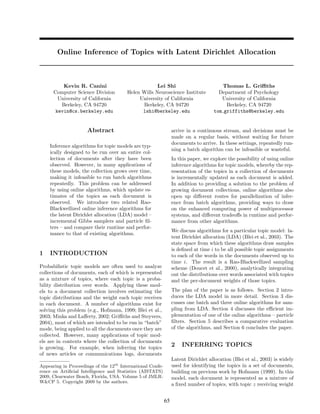
4. Online Inference of Topics with Latent Dirichlet Allocation
ples from the target distribution P (zi |wi ) after each is used after particle resampling to restore diversity
word wi is observed. It does this by first generat- to the particle set in the same way that the incremen-
(p)
ing a value of zi for each particle p from a proposal tal Gibbs sampler rejuvenates its samples, by choosing
(p) (p)
distribution Q(zi |zi−1 , wi ). The prior distribution, a rejuvenation sequence R(i) of topic variables to re-
(p) (p) sample. The length of R(i) can be chosen to trade off
P (zi |zi−1 , wi−1 ), is typically used for the proposal
runtime against performance, and the variables to be
because it is often infeasible to sample from the pos-
(p) (p) resampled can be randomly selected either uniformly
terior, P (zi |zi−1 , wi ). However, since zi is drawn or using a decayed distribution that favors more recent
from a constant, finite set of values, we can use the history, as in Marthi et al. (2002). While a uniform
posterior, which is given by Equation (2) and min- schedule visits earlier sites more overall, using a distri-
imizes the variance of the resulting particle weights bution that approaches zero quickly enough for sites
(Doucet et al., 2000). Next, the unnormalized impor- in the past ensures that in expectation, each site is
tance weights of the particles are calculated using the sampled the same number of times.
standard iterative equation
(p)
ωi
(p) (p)
P (wi |zi , wi−1 )P (zi |zi−1 )
(p) 4 EFFICIENT IMPLEMENTATION
(p)
∝ (p) (p)
(4)
ωi−1 Q(zi |zi−1 , wi )
In order to be feasible as an online algorithm, the par-
(p)
= P (wi |zi−1 , wi−1 ). (5) ticle filter must be implemented with an efficient data
representation. In particular, the amount of time it
The weights are then normalized to sum to 1. Equa- takes to incrementally process a document must not
tion (5) is designed so that after the weight normaliza- grow with the amount of data previously seen. In ini-
tion step, the particle filter approximates the posterior tial implementations of the algorithm, individual par-
distribution over topic assignments as follows: ticles were represented as linear arrays of topic assign-
P
ment values, consistent with the interpretation of the
P (zi |wi ) ≈
(p) (p)
ωi 1zi (zi ), (6) state space zi = (z1 , . . . , zi ) as a sequence of variables
p=1
stored in an array. It was found that nearly all of
the computing time was spent resampling the parti-
where 1zi (·) is the indicator function for zi . As P → cles (line 8 of Algorithm 4). This is due to the fact
∞, the right side converges to the left side, since zi that when a particle is resampled more than once,
can assume only a finite number of values. the na¨ implementation makes copies of the zi ar-
ıve
ray for each child particle. Since these structures grow
Over time, the weights assigned to particles diverge
linearly with the observed data and resampling is per-
significantly, as a few particles come to provide a sig-
formed at a roughly constant rate, the total time spent
nificantly better account of the observed data than the
resampling particles grows quadratically.
others. Resampling addresses this issue by producing a
new set of particles that are more highly concentrated This problem can be alleviated by using a shared rep-
on states with high weight whenever the variance of the resentation of the particles, exploiting the high degree
weights becomes large. A standard measure of weight of redundancy among particles with common lineages.
variance is an approximation to the effective sample When a particle is resampled multiple times, the re-
size, ESS ≈ ω −2 , and a threshold can be expressed sulting copies all share the same parent particle and
as some proportion of the number of particles, P . implicitly inherit its zi vector as their history of topic
assignments. Each particle maintains a hash table that
The simplest form of resampling is to draw from
is used to store the differences between its topic as-
the multinomial distribution defined by the normal-
signments and its parent’s; consequently, the compu-
ized weights. However, more sophisticated resampling
tational complexity of the resampling step is reduced
methods also exist, such as stratified sampling (Kita-
from quadratic to linear. As illustrated in Figure 1,
gawa, 1996), quasi-deterministic methods (Fearnhead,
the particles are thus stored as a directed tree2 , with
2004), and residual resampling (Liu and Chen, 1998),
parent-child relationships indicating the hierarchy of
which produce more diverse sets of particles. Residual
inheritance for topic variables.
resampling was used in our evaluations. Whenever the
(p)
particles are resampled, their weights are all reset to To look up the value zi of topic assignment i in par-
P −1 , since each is now a draw from the same distri- ticle p, the particle’s hash table is consulted first. If
bution and the previous weights are reflected in their the value is missing, the particle’s parent’s hash table
relative resampling frequencies. is checked, recursing up the tree towards the root and
As in the resample-move algorithm of Gilks and 2
More precisely, a forest of directed trees, since it is
Berzuini (2001), Markov chain Monte Carlo (MCMC) possible that not all particles share a common ancestor.
68

5. Canini, Shi, Griffiths
!"#$%&'()*
idence confirms that the time overhead of maintaining
!"#$% &'(# )'*!+
, -.()- / a directed tree of hash tables is negligible compared to
0 -1!2$- / the increase in speed and decrease in memory usage it
/ -3'(.1!)4- 5
5 -!"6'16$7- 0 affords. Specifically, by reducing the resampling step
8 -+9''7!":- 0
; -&9$($- ,
to have linear runtime, this implementation detail is
< -)'- , the key to making the particle filter feasible to run.
= -#(.&- /
> -)9$- ,
? -1!"$- /
5 EVALUATION
In online topic modeling settings, such as news article
!"#$%&'()+ ,-.)!"#$%&'(/
clustering, we care about two aspects of performance:
!"#$% &'(# )'*!+ !"#$% &'(# )'*!+
8 -+9''7!":- 5 , -.()- 0 the quality of the solutions recovered and runtime. As
; -&9$($- 0 8 -+9''7!":- 5 documents arrive and are incrementally processed, we
= -#(.&- 0
would like online algorithms to maintain high-quality
inferences and to produce topic labels quickly for new
documents. Since there is a tradeoff between runtime
!"#$%&'()0 !"#$%&'()1 and inference quality, the algorithms were evaluated
!"#$% &'(# )'*!+ !"#$% &'(# )'*!+ by comparing the quality of their inferences while con-
, -.()- / ; -&9$($- /
? -1!"$- 5 straining the amount of time spent per document. We
compared the performance of the three online algo-
Figure 1: An example of the “directed tree of hashta- rithms presented in Section 3: o-LDA, the incremental
bles” implementation of the particle filter. Particle 2 Gibbs sampler, and the particle filter. Our evaluation
is the root, so all other particles descended from it. is a variation of the comparison of o-LDA to other on-
Particle 0 directly depends on particle 2, altering the line algorithms by Banerjee and Basu (2007), using the
topics of the words “choosing” and “where”. The other same datasets and performance metric.
child of particle 2 is not itself an active sample, but an
inactive remnant of an old particle that was not resam- 5.1 DATASETS
pled. It is retained because multiple active particles
The datasets used to test the algorithms are each a
depend on its hashed topic values. If either particle 1
collection of categorized documents. They consist of
or particle 3 is not resampled in the future, the remain-
four subsets derived from the 20 Newsgroups corpus3 :
ing one will be merged with its parent, maintaining the
(1) diff-3 (2995 documents, 7670 word types, 3 cate-
bound on the tree depth.
gories), (2) rel-3 (2996 documents, 10091 word types,
3 categories), (3) sim-3 (2980 documents, 5950 word
types, 3 categories), and (4) subset-20 (1997 docu-
eventually terminating when the value is found in an ments, 13341 word types, 20 categories), represent-
(p)
ancestor’s hash table. To change the value zi , the ing different levels of size and difficulty, as well as
new value is inserted into particle p’s hash table, and news articles harvested from the Slashdot website: (5)
the old value is inserted into each of particle p’s chil- slash-7 (6714 documents, 5769 word types, 7 cate-
dren’s hash tables (if they don’t already have an entry) gories) and (6) slash-6 (5182 documents, 4498 word
to ensure consistency. types, 6 categories).
In order to ensure that variable lookup is a constant-
time operation, it is necessary that the depth of the 5.2 METHODOLOGY
tree does not grow with the amount of data. This can
Our testing methodology is designed to approximate a
be ensured by selectively pruning the tree just after
real-world online inference task. For each dataset, the
the resampling step. After resampling is performed,
algorithms were given the first 10% of the documents
a node is called active if it has been sampled one or
to use for initialization. A single sample drawn using
more times, and inactive otherwise. If an entire sub-
the batch Gibbs sampler on this initial set was used to
tree of nodes is inactive, it is deleted. If an inactive
initialize all of the online algorithms. This constituted
node has only one active descendant depending on its
the explicit batch initialization phase of o-LDA, and
history, that descendant’s hash table is merged with
the other two online algorithms used the same starting
its own. When this operation is performed after each
configuration.
resampling step, it can be shown that the depth of the
tree is never greater than P . Furthermore, merging the 3
Available online at http://people.csail.mit.edu/
hash tables takes linear amortized time. Empirical ev- jrennie/20Newsgroups/
69

6. Online Inference of Topics with Latent Dirichlet Allocation
After the batch initialization set is chosen, the o-LDA clustered a randomly-chosen held-out set consisting of
algorithm has no remaining parameters and is the 10% of the documents, as a function of the amount of
fastest of the three online algorithms, since it does the training set that had been observed so far. That is,
not rejuvenate its topic assignments. The incremental at regular intervals throughout the training set, each
Gibbs sampler has one parameter: the choice of re- algorithm was run on the held-out documents as if they
juvenation sequence R(i). The particle filter has two were the next ones to be observed, the nMI score was
parameters: the effective sample size (ESS) threshold, calculated for the held-out documents, and the algo-
which controls how often the particles are resampled, rithm was returned to its original state and position
and the choice of rejuvenation sequence. Since the run- in the training set.
time and performance of the incremental Gibbs sam-
pler and the particle filter depend on these parameters, 5.3 RESULTS
there is a compromise to be made. We set the param-
eters so that these algorithms ran within roughly 6 The results of the training set evaluation are shown
times the amount of time taken by o-LDA on each in Figure 2. The particle filter and incremental Gibbs
dataset. For the incremental Gibbs sampler, R(i) was sampler perform about equally well, with the parti-
chosen to be a set of 4 indices from 1 to i chosen uni- cle filter performing better for some datasets. As ex-
formly at random. For the particle filter, the ESS pected, o-LDA consistently has the lowest score of
threshold was set at 20 for the diff-3, rel-3, and the three algorithms. The dashed horizontal line in
sim-3 datasets and at 10 for the subset-20, slash-6, each figure represents the performance of the batch
and slash-7 datasets, |R(i)| was set at 30 for the Gibbs sampler on the entire dataset, which is approx-
diff-3, rel-3, and sim-3 datasets and at 10 for the imately the best possible performance an online algo-
subset-20, slash-6, and slash-7 datasets, and the rithm could achieve using the LDA model.
particular values of R(i) were chosen uniformly at ran- The results of the evaluation on the held-out set are
dom from 1 to i. The runtime of these algorithms can shown in Figure 3. For each held-out set, the mean
be chosen to fit any constraints, but we selected one performance of the particle filter is consistently better
point that we felt was reasonable. Indeed, an impor- than that of the incremental Gibbs sampler, which is
tant strength of these two online algorithms is that consistently better than that of o-LDA. With the ex-
they can take full advantage of any amount of comput- ception of the sim-3 and subset-20 datasets, the al-
ing power by appropriate choice of their parameters. gorithms’ performances are separated by at least two
The LDA hyperparameters α and β were both set to standard deviations. Interestingly, the performance of
be 0.1. The particle filter was run with 100 particles; all the algorithms on all the held-out document sets
to allow the other algorithms the same advantage of does not change significantly as more training data is
multiple samples, they were each run 100 times inde- observed. This seems to indicate that a majority of
pendently, with the sample having highest posterior the information about the topics comes from the first
probability at each step being used for evaluation. 10% of the documents. In rel-3, performance on the
held-out set seems to decrease as more of the training
Since the datasets are collections of documents with set is observed. This could be because the held-out
known category memberships, we evaluated how well documents are more closely related to those at the be-
the clustering implied by the inferred topics matched ginning of the training set than those at the end.
the true categories. That is, for each dataset, the num-
ber of topics T was set equal to the number of cate- As mentioned earlier, the algorithms’ performance
gories, and the documents were clustered according to strongly depends on their parameters; allowing more
their most frequent topic. Normalized mutual infor- time for rejuvenation of old topic assignments would
mation (nMI) was used to measure the similarity of improve the performance of the particle filter and the
this implied partition to the true document categories incremental Gibbs sampler. Table 1 summarizes the
(Banerjee and Basu, 2007). Scores are between 0 and total runtimes of each algorithm on each dataset. Al-
1, with a perfect match receiving a score of 1. though there is some variation, the incremental Gibbs
sampler and particle filter each take about 6 times
Two different evaluations were made for each algo- longer than o-LDA.
rithm on each dataset. First, we evaluated how well
the algorithms clustered the documents on which they The top ten words from 5 of the 20 topics found by the
were trained. That is, at regular intervals through- particle filtering algorithm on the subset-20 dataset
out each dataset, the sample with maximum posterior are listed in Table 2. Although the normalized mutual
probability was drawn, and the quality of the induced information is not as high as that of the batch Gibbs
clustering of the documents observed so far was mea- sampler, the recovered topics seem intelligible.
sured. Second, we evaluated how well the algorithms We also noticed that the particle filter used signifi-
70

7. Canini, Shi, Griffiths
Figure 2: nMI traces for each algorithm on each dataset. The algorithms were initialized with the same config-
uration on the first 10% of the documents. Each dashed horizontal line represents the nMI score for the batch
Gibbs sampler on an entire dataset. Solid lines show mean performance over 30 runs, and shading indicates plus
and minus one sample standard deviation.
Figure 3: nMI traces for each algorithm on held-out test sets, as a function of the amount of the training set
observed. The algorithms were initialized with the same configuration on the first 10% of the documents. Each
dashed horizontal line represents the nMI score on the held-out set for the batch Gibbs sampler given the entire
training set. Solid lines show mean performance over 30 runs, and shading indicates plus and minus one sample
standard deviation.
71

8. Online Inference of Topics with Latent Dirichlet Allocation
Acknowledgements
Table 1: Runtimes of algorithms in seconds. Numbers
in parentheses give multiples of o-LDA runtime. This work was supported by the DARPA CALO project
o-LDA inc. Gibbs particle filter and NSF grant BCS-0631518. The authors thank Jason
diff-3 34 185 (5.4) 183 (5.4) Wolfe for helpful discussions and Sugato Basu for providing
the datasets and nMI code used for evaluation.
rel-3 57 338 (5.9) 251 (4.4)
sim-3 32 176 (5.5) 148 (4.6)
References
subset-20 150 1221 (8.1) 1029 (6.9)
slash-6 44 255 (5.8) 256 (5.8) Banerjee, A. and Basu, S. 2007. Topic models over text
slash-7 69 420 (6.1) 521(7.6) streams: a study of batch and online unsupervised learn-
ing. In Proc. 7th SIAM Int’l. Conf. on Data Mining.
Blei, D. M., Griffiths, T. L., Jordan, M. I., and Tenen-
baum, J. B. 2004. Hierarchical topic models and the
Table 2: The top 10 words from 5 topics found by the nested Chinese restaurant process. In Advances in Neu-
ral Information Processing Systems 16.
particle filter for the subset-20 dataset. Blei, D. M. and Lafferty, J. D. 2005. Correlated topic mod-
els. In Advances in Neural Information Processing Sys-
gun list space god wire tems 18.
police mail cost bible ground Blei, D. M., Ng, A. Y., and Jordan, M. I. 2003. Latent
guns users nasa moral wiring Dirichlet allocation. Journal of Machine Learning Re-
semi email mass choose cable search, 3:993–1022.
Doucet, A., de Freitas, N., and Gordon, N., eds. 2001.
fire internet rockets christian power Sequential Monte Carlo Methods in Practice. Springer.
cops access station jesus neutral Doucet, A., de Freitas, N., Murphy, K. P., and Russell, S. J.
revolver unix orbit church nec 2000. Rao-Blackwellised particle filtering for dynamic
carry address launch christianity circuit Bayesian networks. In Proc. 16th Conf. in Uncertainty
auto security dod absolute box in Artificial Intelligence.
Fearnhead, P. 2004. Particle filters for mixture models
koresh system drink life current with an unknown number of components. Statistics and
Computing, 14(1):11–21.
Gilks, W. R. and Berzuini, C. 2001. Following a mov-
ing target–Monte Carlo inference for dynamic Bayesian
cantly less memory than the other online algorithms. models. Journal of the Royal Statistical Society. Series
This is due to the shared representation of the par- B (Statistical Methodology), 63(1):127–146.
ticles, as discussed in Section 4, which allows more Griffiths, T. L. and Steyvers, M. 2004. Finding scientific
accurate inferences to be computed with less memory topics. Proc. National Academy of Sciences of the USA,
101(Suppl. 1):5228–5235.
than algorithms that maintain independent samples. Griffiths, T. L., Steyvers, M., Blei, D. M., and Tenenbaum,
J. B. 2004. Integrating topics and syntax. In Advances
in Neural Information Processing Systems 17.
6 DISCUSSION Hofmann, T. 1999. Probabilistic latent semantic indexing.
In Proc. 22nd Annual Int’l. ACM SIGIR Conf. on Re-
We have discussed a number of algorithms for the search and Development in Information Retrieval.
problem of inferring topics using LDA. We have shown Kitagawa, G. 1996. Monte Carlo filter and smoother for
non-Gaussian nonlinear state space models. Journal of
how to extend a batch algorithm into a series of Computational and Graphical Statistics, 5(1):1–25.
online algorithms, each more flexible than the last. Liu, J. S. and Chen, R. 1998. Sequential Monte Carlo
Our results demonstrate that these algorithms per- methods for dynamic systems. Journal of the American
form effectively in recovering the topics used in multi- Statistical Association, 93(443):1032–1044.
ple datasets. Latent Dirichlet allocation has been ex- Marthi, B., Pasula, H., Russell, S. J., and Peres, Y. 2002.
Decayed MCMC filtering. In Proc. 18th Conf. in Uncer-
tended in a number of directions, including incorpora- tainty in Artificial Intelligence.
tion of hierarchical representations (Blei et al., 2004), Minka, T. P. and Lafferty, J. D. 2002. Expectation-
minimal syntax (Griffiths et al., 2004), the interests of propagation for the generative aspect model. In Proc.
authors (Rosen-Zvi et al., 2004), and correlations be- 18th Conf. in Uncertainty in Artificial Intelligence.
tween topics (Blei and Lafferty, 2005). We anticipate Rosen-Zvi, M., Griffiths, T. L., Steyvers, M., and Smyth,
P. 2004. The author-topic model for authors and docu-
that the algorithms we have outlined here will natu- ments. In Proc. 20th Conf. in Uncertainty in Artificial
rally generalize to many of these models. In particu- Intelligence.
lar, applications of the hierarchical Dirichlet process to Song, X., Lin, C.-Y., Tseng, B. L., and Sun, M.-T. 2005.
text (Teh et al., 2006) can be viewed as an analogue to Modeling and predicting personal information dissem-
LDA in which the number of topics is allowed to vary. ination behavior. In Proc. 11th ACM SIGKDD Int’l.
Conf. on Knowledge Discovery and Data Mining.
Our particle filtering framework requires little modifi- Teh, Y. W., Jordan, M. I., Beal, M. J., and Blei, D. M.
cation to handle this case, providing an online alter- 2006. Hierarchical Dirichlet processes. Journal of the
native to existing inference algorithms for this model. American Statistical Association, 101(476):1566–1581.
72