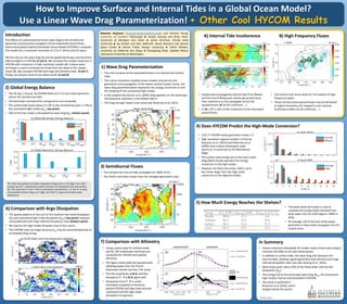
1. How to Improve Surface and Internal Tides in a Global Ocean Model?
Use a Linear Wave Drag Parameterization! + Other Cool HYCOM Results
Introduction
The effects of a parameterized linear wave drag on the semidiurnal
barotropic and baroclinic energetics of the realistically forced three-
dimensional global Hybrid COordinate Ocean Model (HYCOM) is analyzed.
The model has a horizontal resolution of 1/12.5 (8 km) and 32 layers.
We first discuss the wave drag (1) and the global barotropic and baroclinic
tidal energetics in HYCOM (2 and 3). We compare the modal conversion in
HYCOM with conversion in high resolution models (4). A plane-wave
technique is used to estimate the fluxes from the deep to the coastal
ocean (5). We compare HYCOM with Argo and altimetry data. (6 and 7).
Finally, we present some of our latest results (A and B).
Maarten Buijsman (maarten.Buijsman@usm.edu) and Victoria Young,
University of Southern Mississippi  Joseph Ansong and Brian Arbic,
University of Michigan Ann Arbor  James Richman, Florida State
University  Jay Shriver and Alan Wallcraft, Naval Research Lab Stennis
Space Center  Patrick Timko, Bangor University  Caitlin Whalen,
University of California San Diego  Zhongxiang Zhao, Applied Physics
Laboratory University of Washington
In Summary
• Coarse resolution tidal global 3D models need a linear wave drag to
minimize SSH RMS errors with observations.
• In addition to surface tides, the wave drag also dampens the
internal tides, yielding a good agreement with altimetry and Argo
inferred dissipation rates (see also Ansong et al., 2015).
• Wave drag causes about 50% of the deep water internal tide
dissipation (Dwl).
• The energy lost to the barotropic wave drag (Dw0, the unresolved
high modes) may be overestimated in HYCOM.
• This work is published in
Buijsman et al (2016), which
dangles below this poster.
7) Comparison with Altimetry
PO34C-3078
1) Wave Drag Parameterization
• The main purpose of the parameterization is to improve the surface
tides.
• The coarse resolution of global ocean models only permits the
generation and propagation of the lowest vertical modes; hence, the
wave drag parameterization represents the energy conversion to and
the breaking of the unresolved high modes.
• In this analysis the Garner et al. (2005) drag operates on the barotropic
and baroclinic velocities in the bottom 500 m.
• The drag strength needs to be tuned (see Buijsman et al, 2015).
3) Semidiurnal Fluxes
• The semidiurnal internal tides propagate for 1000s of km.
• The Pacific and Indian ocean have the strongest generation sites.
6) Comparison with Argo Dissipation
• The spatial patterns of the sum of the resolved low-mode dissipation
(Dl) and unresolved high-mode dissipation (Dw0) (top panel) compare
reasonably well with Argo-inferred dissipation rates (bottom panel).
• We assume the high modes dissipate close to the source.
• The HYCOM rates are larger because Dw0 may be overestimated due to
incomplete drag tuning.
2) Global Energy Balance
• The 30-day, 1-hourly, 3D HYCOM fields are 9-15 hour band-passed to
extract the semidiurnal tides.
• The barotropic and baroclinic energy terms are computed.
• The surface tide looses about 0.5 TW to the resolved low and 1.2 TW to
the unresolved high modes (Dw0, top panel).
• 50% of the low modes is dissipated by wave drag (Dwl, bottom panel).
The tidal-mean global and depth-integrated energy terms in the figure are: tidal
energy input (P) , resolved low-mode conversion (C), dissipation (D), and residual
(R). The subscripts ‘0’ and ‘l’ refer to barotropic and baroclinic, ‘w’ and ‘b’ to wave
and quadratic bottom drag, and ‘ridge’ and ‘shelf’ to deep and shallow water
bathymetry.
(a) (b)
(c) (d)
polewardequatorward• Using a plane-wave fit method mode-
one M2 SSH amplitudes and fluxes are
computed for HYCOM and satellite
Altimetry.
• The figure shows pole and equatorward
radiating waves from the French
Polynesian Islands (see box 3 for area).
• The SSH amplitudes (a & b) and flux-
divergence ∇ ∙ 𝐅 (c & d) agree well.
• Dissipation from ∇ ∙ 𝐅 is under-
estimated compared to the band-
passed HYCOM and Argo rates because
conversion and the high-mode
dissipation are ignored.
4) Does HYCOM Predict the High-Mode Conversion?
• 1/12.5 HYCOM mainly generates modes 1-3
• High resolution regional models (<2 km) by
Buijsman et al. (2014) and Zilberman et al.
(2009) have a better developed mode
spectrum, in particular at the Mid Atlantic
Ridge
• The surface tidal energy lost to the linear wave
drag (Dw0) should represent the energy
conversion to the high modes.
• However, for these two areas, Dw0 is up to
four times larger than the high mode
conversion in the regional models.
5) How Much Energy Reaches the Shelves?
• The plane-wave technique is used to
compute the energy fluxes directed from
deep water into the shelf regions <4000 m
deep.
• On average 12% of the low-mode waves
generated in deep water propagate into the
coastal areas.
B) High Frequency FluxesA) Internal Tide Incoherence
• Equatorward propagating internal tides from Hawaii
and the French Polynesian Islands (a) quickly loose
their coherence as they propagate across the
equatorial jets (b) (to be continued ….).
• In (b) 1-R2 is ratio of the incoherent to the total band-
passed fluxes.
P
H
• One-hourly time series allow for the analysis of high-
frequency waves.
• These 3-8 hour band-passed fluxes may be attributed
to higher harmonics of f, trapped in anti-cyclonal
Gulfstream eddies (to be continued ….).