
Recomendados
Mais conteúdo relacionado
Mais procurados
Mais procurados (19)
Semelhante a How Analytic Reporting Can Identify and Solve Paratransit Service Shortcomings
Semelhante a How Analytic Reporting Can Identify and Solve Paratransit Service Shortcomings (20)
Último
Último (20)
How Analytic Reporting Can Identify and Solve Paratransit Service Shortcomings
- 1. How Analytic Reporting Can Identify and Solve Paratransit Service Shortcomings Will Rodman VP, Business Development TSS Paratransit
- 2. Let’s Start at the Beginning A goal of most paratransit systems: to minimize unit costs while maintaining service standards. What is the “right” balance of Cost Efficiency (CE) and Service Quality (SQ) for your system. 2 SQ SQ SQ CE CE CE
- 3. 3 Achieving the Optimal Balance btw Cost Efficiency and Service Quality Cost efficiency measured in cost per trip Cost efficiency mostly derived from: Competitive service provider rates and incentives Productive schedules; reducing miles thru shared-rides Run structures that mirror demand profile Strategic use of non-dedicated service providers SQ CE A truism: The tighter the schedule, the more OTP is reduced.
- 4. 4 Achieving the Optimal Balance btw Cost Efficiency and Service Quality Cost efficiency measured in cost per trip Cost efficiency mostly derived from: Competitive service provider rates and incentives Productive schedules; reducing miles thru shared-rides Run structures that mirror demand profile Strategic use of non-dedicated service providers SQ CE A truism: The tighter the schedule, the more OTP is reduced.
- 5. What is a Run Structure? 5 5 6 7 8 9 10 11 12 1 2 3 4 5 6 Serv Hrs Pay Hours 1 1 1 1 1 1 1 1 1 8 9 2 1 1 1 1 1 1 1 1 8 9 3 1 1 1 1 1 1 1 7 9 4 1 1 1 1 1 1 1 7 9 5 1 1 1 1 1 1 1 7 9 6 1 1 1 1 1 1 1 7 9 7 1 1 1 1 1 1 1 7 9 8 1 1 1 1 1 1 1 7 9 0 2 2 8 8 6 3 3 6 8 8 2 2 0 58 72 8 7 6 5 4 3 2 1 5 6 7 8 9 10 11 12 1 2 3 4 5 6
- 6. What is a Demand Profile? 6 Graph of trips per hour for each hour or half hour of the service day Superimpose demand profile on run structure based on current productivity
- 7. Run Structure vs. Demand Profile 7 Tuesday (10-5-04) - Ridership and Capacity 0 5 10 15 20 25 30 4 5 6 7 8 9 10 11 12 1 2 3 4 5 6 7 8 9 10 11 12+ Time of Day Runs 0 10 20 30 40 50 60 Trips Template Runs Actual Runs Ridership
- 8. Case Study #1 8 Addressing a Suboptimal Run Structure
- 9. Case Study #1: The Problem 9 OTP really low overall OTP really low in afternoon (54-82%) Not enough supply of service in the afternoon Could existing run start times be shifted to increase supply of service in the afternoon?
- 10. Case Study #1: The Guidleines 10 Short-term band aids needed until runs re-bid Increase the capacity between the hours of 13:00 and 19:00, when OTP is the lowest. Minimize number of runs impacted Focus: shift runs from oversupply periods Cost neutral solutions Band Aid #1: Shift runs w/o adjusting run length Band Aid #2: Shift runs with length adjustments
- 11. Before OTP – Week of 6/12/17 Trip Type On-Time Percentage ADA Paratransit Trips 84.94% Premium Trips 86.69% 11 OTP in Afternoon = 54% to 82%
- 12. BA #1: Shift Run Start Times Only 12 What do we notice? Over-supply <9:00 am >3:00 pm Under-supply 9:00-noon 1:00-3:00 BA #1 solution (blue) - addresses problem time
- 13. BA #2: Start Times & Adjustments 13 Extended some AM shifts from 8 to 10 hours More capacity added from noon to 6 pm OTP problem in afternoon addressed
- 14. Before and After OTP Trip Type OTP Week of 6/12/17 OTP Week of 11/6/17 ADA Para Trips 84.94% 90.86% Premium Trips 86.69% 94.99% 14
- 15. Before and After Productivity Trips - Week of 6/12/17 Trips - Week of 9/25/17 Before Productivity After Productivity Monday 2053 2082 (1.4%) 1.434 1.504 (4.9%) Tuesday 2329 2351 (0.9%) 1.485 1.539 (3.6%) Wednesday 2384 2455 (3.0%) 1.479 1.537 (3.9%) Thursday 2429 2435 (0.2%) 1.497 1.567 (4.7%) Friday 2075 1975 (-4.8%) 1.456 1.534 (5.4%) 15 Productivity increases = 3.6% to 5.4%
- 16. Before and After and After OTP Trip Type OTP Week of 6/12/17 OTP Week of 11/6/17 OTP Week of 2/5/18 ADA Para Trips 84.94% 90.86% 94.72% Premium Trips 86.69% 94.99% 95.17% 16
- 17. Optimization Tools Temporal/geographic analysis of accommodated demand, unassigned trips Filters to perform analyses of providers, fleets, vehicle types, service areas, days/times, dedicated vs. non-dedicated service providers Detail and summary (various subgrouping) of scheduling results Individual itinerary assessment 17
- 18. Optimization Tools (continued) Provides the ability to: Modify run structure and forecast results Assess impact of seasonal parameters Assess impact of changing scheduling or on- time windows, provider cost, veh. capacity, changes in service zones, transfer points As input, any previously recorded scheduling snapshot can be loaded in and analyzed 18
- 19. Metrics and More Metrics Number of Vehicles (Resources) Available, Used (Needed) and Utilization Number of Revenue Vehicle Hours Driver Regular Hours – Available, Used Driver Overtime Hours – Available, Used Idle Time, Dwell Time, Deadhead Time Average Productivity – Trips per RVH, Direct Miles per RVH 19
- 20. Metrics and More Metrics (cont’d) Percentage of Shared Trips Average Distance – Total and Direct Average Travel Time – Total and Direct Average Speed – Total and Direct Trips Assigned – Total, amb, w/c Trips Unassigned – Total, amb, w/c Percentage of On-Time and Late Trips Cost per trip, cost per RVM 20
- 21. Active & Inactive Service Supply 21
- 23. Strategies / Simulations 1 Adjusted Start Times; Run Lengths Unchanged 2 Eliminated Zones and Inter-Zone Transfers 3 Scenarios 1+ 2 4 Scenario 3 plus 15% cancellations 5 Scenario 4; 10% advance + 5 % late/no-shows 6 Scenario 5 plus NDSPs 23
- 24. The Results Scenario Vehicles Productivity Cost Per Trip Unassigned Base 645 1.47 $33.96 358 1 645 1.49 $31.61 152 2 645 1.49 $33.63 326 3 645 1.49 $33.46 6 4 603 1.32 $37.91 -- 5 572 1.42 $35.17 36 6 653/33 1.43 $34.69 -- 24 Scheduling Tests Scheduling Tests and Simulations 1 Adjusted Start Times 4 Scenario 3 plus 15% cancellations 2 Eliminated Zones/Transfers 5 Scenario 4; 10% adv + 5% lates/NS 3 Scenarios 1+ 2 6 Scenario 5 plus NDSPs
- 25. Case Study #2 25 Addressing a Suboptimal Service Mix
- 26. Case Study #2: Run Structure vs. Demand Profile - October 2004 26 Tuesday (10-5-04) - Ridership and Capacity 0 5 10 15 20 25 30 4 5 6 7 8 9 10 11 12 1 2 3 4 5 6 7 8 9 10 11 12+ Time of Day Runs 0 10 20 30 40 50 60 Trips Template Runs Actual Runs Ridership
- 27. 27 0 5 10 15 20 25 30 35 40 45 50 Monday Vehicles in Service vs. Vehicles Required by Time Period Vehicles in Service Vehicles Required Active Vehicles 0 5 10 15 20 25 30 35 40 45 50 Tuesday Vehicles in Service vs. Vehicles Required by Time Period Vehicles in Service Vehicles Required Active Vehicles 0 5 10 15 20 25 30 35 40 45 50 Wednesday Vehicles in Service vs. Vehicles Required by Time Period Vehicles in Service Vehicles Required Active Vehicles 0 5 10 15 20 25 30 35 40 45 50 Thursday Vehicles in Service vs. Vehicles Required by Time Period Vehicles in Service Vehicles Required Active Vehicles 0 5 10 15 20 25 30 35 40 Friday Vehicles in Service vs. Vehicles Required by Time Period Vehicles in Service Vehicles Required Active Vehicles Case Study #2: Run Structure vs. Demand Profile – May 2012
- 28. Case Study #2: Run Structure Optimization Test – May 2012 28 Weekly Total Vehicle Hours Weekly Driver Hours Max Vehicles in Service Existing 2704 2887 52 Optimized 2674 2850 51 Difference -1.1% -1.3% -1.9%
- 29. Case Study #2: Service Mix Analysis - May 2012 29 Diverting peak period trips had diminishing returns. Why? Because weekday dedicated run structures were close to optimal Diverting trips to NDSPs during low-demand times (evenings and weekends) produced the most savings
- 30. Alternative Services 30 Predicting ridership needed to reduce overall cost Predicting subsidy per trip needed to reduce overall cost At what point do the savings from diverted trips exceed the additional subsidy paid out for new trips generated
- 31. The Bet: What’s the Break Even Point? 31
Notas do Editor
- Good morning. Thank you for that nice introduction. Most of you know me from 40 years at Multisystems and Nelson\Nygaard where a large focus of my practice was helping transit systems with their paratransit services and eking out higher productivities where possible. Two mistakes that I discovered over and over again, and this had nothing to do with what software they were using, was that that (1) they had failed to establish a paratransit run structure that mirrors the demand profile, and (2) they were not taking advantage of opportunities to use non-dedicated service providers in an integrated fashion to reduce unit cost. And so today, I will provide some examples showing how these strategies are suggested through standard analytic reports and new optimization tools that optimize run structures and service mixes. And if there is time, I will also show you a simple way to evidence cost reduction from yet another strategy: that being the implementation of an “Alternative Service” such as a supplemental taxi/TNC subsidy programs for ADA paratransit customers.
- So, to quote Julie Andrews from the Sound of Music, let’s start at the very beginning, a very good place to start. While every paratransit system has their own sense of what the balance between cost efficiency and service quality should be, they don’t use that as the driving force for designing their service or shaping their RFP and contracts; and more often, it’s the other way around.
- If we focus on the cost efficiency side of the see-saw, we see that cost efficiency is mostly derived from: service provider rates and incentives and penalties (for those systems which use operations contractors) Productive schedules, where a maximized number of shared rides help to reduce miles traveled A run structure that mirrors the demand profile, and Strategic use of NDSPs
- Today, we are going to focus on how analytic tools and reporting can help you with the last two.
- A run structure is simply the graph of your available dedicated resources (vehicles). If you software system doesn’t already produce this for you, it’s pretty easy to graph each run, stick a “1” in each cell, add up the cells, and put together a bar graph. The bar graph then is your run structure. In this example, the orange time consists of the pre-trip, lunch breaks, and the post trip time when the vehicle is unavailable for service. So, the yellow, in a sense is portraying garage out to garage in time less scheduled breaks. We also see that the first two runs are split shifts. The result is a two humped run structure that often mirrors the demand profile.
- Meanwhile, the demand profile is a line graph of the trips per hour -- or per half hour of you want to portray it more finely. So, the trick is to superimpose the demand profile over the run structure to see how closely they match.
- Here’s one that I did years ago, the bar charts are the scheduled an actual runs and the line is the demand profile. So, if you were all consultants, what would be your conclusion. Not enough resources in the peak periods, and too much service in the off-peak mid-day and evening periods. The solution is to shift some resources from when they are not needed to when they are needed. And this is what happened in our first case study.
- In a large paratransit system I was helping, the system was plagued with a low overall OTP, but it was really low in the afternoon Upon superimposing the run structure on the demand curve, it became abundantly clear that there was not enough service in the afternoon. So, the paratransit manager asked me to see if any runs could be shifted from over supply periods to supply more service in the afternoon. The concept was meant to be a band aid up until a new more optimal run structure could be created and bid-out.
- Here were the ground rules for the analysis Our goal was to increase the capacity at times when the OTP was the lowest Minimize the number of shifted runs, but as a strategy, focus on shifting runs from the over-supply periods And, the result had to be cost-neutral. So, we actually attempted two band-aids: one that did not involve adjusting the run length and one that did.
- Here was a starting point. This is what we had to improve.
- So, in Excel, we first shifted some run starts times from the oversupply times to the under supply time. This was Band-Aid #1. Here, the dotted line is the demand profile, the solid gray line is the before run structure and the blue line is the after run structure after the shifting. So, you probably would expect some improvement not on only in productivity but in OTP as well because there are more resources available when they are needed.
- In Band-Aid #2, we also were allowed to modify the length of runs to see if we could eke out any more productivity. Here, the yellow line is the band aid one line and the solid blue line is the band aid 2 line, and you see that solid blur line does a pretty fair job addressing the second afternoon hump in the demand profile.
- So, a version of Band Aid 2 was implemented, and the results were that OTP improved significantly.
- And productivity increased as well by 3.6% to 5.4%, depending on the day of the week.
- Moreover, another “after” period showed that OTP improved even more.
- Now, I did that all with Excel. There are now tools available with some paratransit software systems, such as ours, that provide tools for optimizing run structures, but these optimization tools provide so much more. For example, you can change the times of one run or more than one run, press a button and a report will instantly tell you how the change has impacted productivity and cost and other service quality metrics. Moreover, you can leave all of your resources unscheduled, and it will optimize them for you.
- The tools allow you to take a snapshot of any previous schedule, and make other changes as well and then instantaneously see the impact. For example, you can make a policy change (pick-up window), or change a zone boundary, or introduce a fleet with a new capacity configuration, or introduce a defined level of NDSP, and boom, you will see the results in seconds. Oh how I used to spend hours and sometime days figuring this out as a consultant, and now it does it seconds. It’s very cool.
- And here is a partial list of the metrics for which the impacts are measured.
- But wait, there’s more!
- But beyond the what-if planning, this tool can also be used to analyze a problem, much like I formerly did in Excel. Here is the first of two graphs that illustrate the same kind of problem I introduced earlier but in much greater detail and generates the graph in seconds. So this graph focuses on one of the service providers from that system I was helping, and this particular provider had an excess service supply of service in the morning and an insufficient service supply in the afternoon. So, in this first graph, the yellow portion reflects vehicles actively engaged in serving trips, the purple is unutilized time at the beginning of a shift, and brown is the unutilized time at the end of a shift, and the gray indicates breaks.
- The second graph shows the same problem but in a different way. It shows unassigned trips per hour. So, this graph shows that there were a significant number of trips in the afternoon that the software was unable to assign. Why? Because there was not enough supply of service in the afternoon.
- Here are example of optimization scenarios you can run that again used to take me hours if not days.
- And this table shows you just a few of the results.
- Now in the second case study, we present another optimization tool that can focus on service mix.
- Remember this graph from the very beginning of the presentation.
- Well, damned if they didn’t take my advice, and when I ran an analysis, I couldn’t improve upon the weekday service much. You see, they had implemented the suggested changes from the first study, for each day of the week the graphs show how closely their run revised structure matched their demand profile.
- So the conclusion when we ran the optimization software was there wasn’t a whole lot we could do.
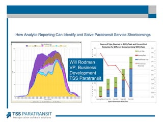
- And because the runs were so optimal, the introduction of NDSPs during the peak periods would actually end up costing them more. On the graph the descending red line is the savings, and what the graph shows is that the optimal savings was when NDSPs are intriduced in the low-demand periods on weekday evenings and on the weekends, and that became their marching orders.
- I also mentioned at the very beginning that we would spend a little time talking about alternative services such as taxi subsidy programs designed to provide non-ADA paratransit on-demand services for ADA paratransit customers. Taxi-based examples of alternatives services have existed for years in cities like Chicago, Denver, and Houston, while newly minted versions involving TNCs have been popping up in cities like Boston and Las Vegas. And we know that transit agencies have two goals in mind as they implement alternative services and pilots: the first is to provide an on-demand mobility option to ADA paratransit customers, and the second is to reduce over-all paratransit costs. So, in the planning of such services, it becomes worthwhile to figure what level of ridership and subsidy levels will help transit agencies figure out whether they have achieved that second goal. I often refer to this as winning the financial bet: that is, at what point do the savings from diverted trips exceed the additional subsidy paid out for new trips generated.
- So, in this example, the subsidy level of the ADA paratransit service is three times the agency-established subsidy level for the new alternative service, noting that a transit agency can really establish the subsidy at any level. And so with this particular example, if less than 2 new trips are generated for each diverted ADA paratransit trip, the transit agencies lowers its overall paratransit cost. If more than 2 new trip are created, the cost of the new service increases the overall paratransit cost You will note that this is a simple model, and does not account for any gains or losses in productivity and associated unit cost of the dedicated fleet that results from trip diversion. But I’m working on it. Otherwise how do you know if a trip would really have otherwise been taken on the ADA paratransit service? If you know who is travelling, you can look at their before and after trip history on the ADA paratransit service and the new alternative service to estimate how many are diverted trips and how many are new trips. So to get that data, you need to either contractually require the service providers to provide data for each client, or you can create a model where requests for the alternative service must come through a central call center, as they do in Denver and Dallas. And in places like Boston, they have also limited the use of alternatives services based on your trip history, thereby increasing the chance that the MBTA will win their financial bet. And in one case that I have seen, customer service representatives (aka reservationists) pose the offer immediately after an ADA paratransit trip has been booked. This was in NYC where they were doing this for certain trips. In NYC, CSRs are permitted to extend a similar offer in the case of stranded riders.
- So, that’s my presentation. I hope you have found it useful or at least interesting. Here’s my actual size business card if you need to ask any questions when you are back at the ranch. Please feel free to call. Thanks you very much.