This document provides notes from a 1996 short course on modern grid generation techniques. It discusses the history and current state of grid generation, as well as mathematical foundations and numerical techniques for generating 2D and 3D grids. Specific techniques covered include generating grids for complex geometries using a multiblock approach, local grid clustering using "clamp" mappings, and grid adaptation. The document also proposes a grid generation meta-language and examines tools for automatic topology definition and parallelization strategies.

1. COSMASE Shortcourse Notes
EPF Lausanne 1996
Modern Introduction to
Grid Generation
Jochem H¨ userc
a
Yang Xia
Department of Parallel Computing
Center of Logistics and Expert Systems
Salzgitter, Deutschland
­
c Jochem H¨ user
a
All Rights Reserved
Notes prepared for COSMASE Shortcourse in Grid Generation
EPF Lausanne, 23-27 September 1996

2. Contents
1.0 Overview and Status of Modern Grid Generation . . . . . . . . . . . . . . . 1
2.0 Methods of Differential Geometry in
Numerical Grid Generation . . . . . . . . . . . . . . . . . . . . . . . . . . . . 3
3.0 Introduction and Overview of Numerical
Grid Generation Techniques . . . . . . . . . . . . . . . . . . . . . . . . . . . . 9
3.0.1 General Remarks on Grid Generation
Techniques . . . . . . . . . . . . . . . . . . . . . . . . . . . . . . . . . 9
3.0.2 A Short History on Grid Generation . . . . . . . . . . . . . . . . . . . 9
3.0.3 What Is a Good Grid . . . . . . . . . . . . . . . . . . . . . . . . . . . . 13
3.0.4 Aspects of Multiblock Grid Generation . . . . . . . . . . . . . . . . . . 14
3.1 Equations of Numerical Grid Generation . . . . . . . . . . . . . . . . . . . . . 16
3.1.1 Elliptic Equations for 2D Grid Generation . . . . . . . . . . . . . . . . 16
3.1.2 Elliptic Equations for Surface Grid Generation . . . . . . . . . . . . . 19
3.1.3 Elliptic Equations for 3D Grid Generation . . . . . . . . . . . . . . . . 23
3.2 Grid Generation Concepts . . . . . . . . . . . . . . . . . . . . . . . . . . . . . 25
3.2.1 Computational Aspects of Multiblock Grids . . . . . . . . . . . . . . . 25
3.2.2 Description of the Standard-Cube . . . . . . . . . . . . . . . . . . . . . 26
3.2.3 The Grid Grid Generation Toolbox . . . . . . . . . . . . . . . . . . . 30
3.2.4 Input for Grid Generation in 2D and 3D . . . . . . . . . . . . . . . . . 31
i

3. 3.2.4.1 Rectangle Grid Example . . . . . . . . . . . . . . . . . . . . 32
3.2.4.2 Diamond Shape 6 Block Grid Example . . . . . . . . . . . . 33
3.3 Local Grid Clustering Using Clamp Technique . . . . . . . . . . . . . . . . . . 41
3.3.1 Hyperboloid Flare in F4 Windtunnel Grid . . . . . . . . . . . . . . . . 43
4.0 Grid Adaptation Techniques . . . . . . . . . . . . . . . . . . . . . . . . . . . . 47
4.0.1 Adaptation by Controlfunctions . . . . . . . . . . . . . . . . . . . . . 48
4.0.2 Algebraic Adaptation Algorithms . . . . . . . . . . . . . . . . . . . . . 52
5.0 A Grid Generation Meta Language . . . . . . . . . . . . . . . . . . . . . . . . 59
5.0.1 Topology Input Language . . . . . . . . . . . . . . . . . . . . . . . . . 59
5.0.2 TIL Code for the Cassini-Huygens
ConÞguration . . . . . . . . . . . . . . . . . . . . . . . . . . . . . . . 71
5.0.2.1 TIL Code for 6 Block Cassini–Huygens Grid . . . . . . . . . 71
5.0.2.2 TIL Code for 24 Block Cassini–Huygens Grid . . . . . . . . 73
5.0.3 TIL Topology and Grid Quality . . . . . . . . . . . . . . . . . . . . . . 74
6.0 Tools for Automatic Topology DeÞnition . . . . . . . . . . . . . . . . . . . . . 79
6.0.1 Example Topology 1: A Circle in a Box . . . . . . . . . . . . . . . . . . 80
6.0.2 Example Topology 2: Two Circles in a Box . . . . . . . . . . . . . . . . 93
6.0.3 Example Topology 3: Cassini–Huygens Space Probe . . . . . . . . . . 99
7.0 Parallelization Strategy for Complex Geometries . . . . . . . . . . . . . . . . 102
7.0.1 The Abstract Parallel Machine . . . . . . . . . . . . . . . . . . . . . . 102
7.0.2 General Strategy . . . . . . . . . . . . . . . . . . . . . . . . . . . . . . 103
7.0.3 Encapsulation of Message Passing . . . . . . . . . . . . . . . . . . . . 103
7.0.4 Aspects of Software Engineering: C versus Fortran . . . . . . . . . . . 105
7.0.5 Numerical Solution Strategy: A Tangled Web . . . . . . . . . . . . . . 106
ii

4. List of Figures
2.1 Curvilinear nonorthogonal Coordinate System. The contravariant base vectors e i
ˆ
point in the tangential directions but are not unit vectors. Vectors ei are Cartesian
unit vectors. . . . . . . . . . . . . . . . . . . . . . . . . . . . . . . . . . . . . . 3
3.1 In this chart the complete modelization process starting from the surface descrip-
tion of the vehicle, coming from the design ofÞce, to the visualized results of a 3D
ßow solution is depicted. The necessary data Þles along with the corresponding
software modules are shown. . . . . . . . . . . . . . . . . . . . . . . . . . . . . 11
3.2 Standard cube in CP (computational plane). Each cube has its own local coordinate
system. The grid is uniform in the CP. . . . . . . . . . . . . . . . . . . . . . . . 26
3.3 Mapping of a block from SD to CP. Arrows indicate orientation of faces, which
are numbered in the following way: 1 bottom, 2 front, 3 left, 4 right, 5 back, 6 top.
The rule is that plane ζ 1 corresponds to 1, plane η 1 to 2 and plane ξ 1 to 3. 27
3.4 Orientation of faces. Coordinates ξ, η, ζ are numbered 1, 2, 3 where coordinates
with lower numbers are stored Þrst. . . . . . . . . . . . . . . . . . . . . . . . . . 28
3.5 Determination of orientation of faces between neighboring blocks. . . . . . . . . 28
3.6 The Þgure shows the overlap of two neighboring blocks. . . . . . . . . . . . . . 29
3.7 The 8 possible orientations of neighboring faces are shown. Cases 1 to 4 are ob-
tained by successive rotations e.g. 0, 1 π, π and 3 π. The same situation holds for
2 2
cases 5 to 8. . . . . . . . . . . . . . . . . . . . . . . . . . . . . . . . . . . . . . 29
3.8 A 6 block grid for diamond shaped body. This type of grid line conÞguration
cannot be obtained by a mono-block grid. . . . . . . . . . . . . . . . . . . . . . 35
3.9 Grid line can also be clustered to match the physics of the ßow; e.g. resolving a
boundary layer. . . . . . . . . . . . . . . . . . . . . . . . . . . . . . . . . . . . 35
3.10 Control information for the 6 block diamond grid. This command Þle is also used
by the parallel ßow solver. ÒÞle diamond contains the actual coordinate values. . 36
iii

5. 3.11 Coordinate values of the Þxed (physical) boundaries of the 6 block diamond grid. 37
3.12 So called clamp technique to localize grid line distribution. The real power of this
technique is demonstrated in the Hyperboloid Flare in F4 Windtunnel grid. . . . 41
3.13 Clamp 1 at hyperboloid ßare. . . . . . . . . . . . . . . . . . . . . . . . . . . . . 41
3.14 Clamp 2 at hyperboloid ßare. . . . . . . . . . . . . . . . . . . . . . . . . . . . 42
3.15 A conventional topology for a hyperboloid ßare in a windtunnel. Although the
topology allows a reÞnement of the grid from an Euler to a N–S grid, this re-
Þnement extends into the far Þeld and thus causes a substantial computational
overhead. Numbers denote block numbers, doted lines are block boundaries, solid
lines are grid lines. . . . . . . . . . . . . . . . . . . . . . . . . . . . . . . . . . 43
3.16 Topology of 36 block hyperboloid ßare. This topology is one part of the topology
of 284 block grid, see Fig. 3.18. . . . . . . . . . . . . . . . . . . . . . . . . . . 44
3.17 36 block grid for hyperboloid ßare. . . . . . . . . . . . . . . . . . . . . . . . . 45
3.18 Topology of 284 block grid for hyperboloid ßare in windtunnel. . . . . . . . . . 45
3.19 284 block grid for hyperboloid ßare in windtunnel. . . . . . . . . . . . . . . . . 46
4.1 1 block adptive grid for supersonic inlet, adapted by control functions. . . . . . . 50
4.2 3 block adaptive grid for forward facing step, adapted by control functions. . . . 51
4.3 One–dimenisional monitor surface (MS). The initial grid in the physical SD is
uniform. Lifting up the grid points produces the grid on the monitor surface. The
variable s denotes arc lehgth on the MS . . . . . . . . . . . . . . . . . . . . . . 52
4.4 Repostioned grid on the monitor surface. Grid points are uniformly distributed on
the monitor surface so that arc length spacing is constant. When projected down
back to the physical solution domain, this results in a clustering according to the
gradient of the monitor surface. . . . . . . . . . . . . . . . . . . . . . . . . . . . 52
4.5 Repositioning of grid points on the monitor surface according to the magnitude of
curvature, resulting in a clustering of grid points to regions where curvature κ 0. 53
4.6 Adaptation of a grid using the monitor surface technique to capture a moving
shock together with a strong circular gradient (vortex). The initial grid has uniform
grid spacing. . . . . . . . . . . . . . . . . . . . . . . . . . . . . . . . . . . . . . 56
5.1 Navier-Stokes grid for a four-element airfoil, comprising 79 blocks.The Þrst layer
of grid points off the airfoil contour is spaced on the order of 10 6 based on chord
length. . . . . . . . . . . . . . . . . . . . . . . . . . . . . . . . . . . . . . . . . 60
iv

6. 5.2 The Þgure shows the block structure of the four element airfoil generated by
GridPro. . . . . . . . . . . . . . . . . . . . . . . . . . . . . . . . . . . . . . . 61
5.3 Grid for a T joint that has numerous industrial applications. . . . . . . . . . . . . 61
5.4 Sphere in a torus. The input for this grid is presented in the following tables. . . . 62
5.5 Complete 3D grid for a generic aircraft with ßaps, constructed from analytical
surfaces. However, the topology is exactly the same as for a real aircraft. . . . . . 62
5.6 The picture shows a blowup of the engine region of the generic aircraft.Future
TSTO or SSTO vehicles will exhibit a similar complex geometry, necessitating
both the modelization of internal and external ßows. . . . . . . . . . . . . . . . . 63
5.7 . . . . . . . . . . . . . . . . . . . . . . . . . . . . . . . . . . . . . . . . . . . 63
5.8 . . . . . . . . . . . . . . . . . . . . . . . . . . . . . . . . . . . . . . . . . . . 64
5.9 Topological design for the Huygens space probe grid. In this design all elements,
such as SSP, GCMS and sensors are ignored. . . . . . . . . . . . . . . . . . . . 72
5.10 The 6 block Huygens grid is depicted. It is bounded by a large spherical far Þeld,
in which the Huygens space probe is embedded. The ratio of the far Þeld radius
and the Huygens radius is about 20. . . . . . . . . . . . . . . . . . . . . . . . . 75
5.11 Illustration of the block topology for the 24 block Huygens grid. Left: Topology
top view. The far Þeld, the Huygens body and GCMS are clamped by quads. Right:
Topology side view. Again clamps are used for the 3D topological design. . . . . 75
5.12 24 block grid for Huygens space probe including SSP. . . . . . . . . . . . . . . 76
5.13 Topological description for a two–loop hyperquad is depicted. Some attention has
to be given to the placement of the wireframe points. In both cases, the topology
remains unchanged while wireframe corners are different. It is obvious that in the
second case an overlap is encountered and grid lines will be folded. . . . . . . . 77
5.14 The wireframe should reßect the actual geometry. Although wireframe coordinates
are not Þxed, a better initial solution will lead to faster convergence and inproved
grid quality. . . . . . . . . . . . . . . . . . . . . . . . . . . . . . . . . . . . . . 77
5.15 The grid quality is inßuenced by the initial coordinate values of the wireframe
corners A distorted wireframe may cause grid skewness and folded lines. . . . . 78
6.1 In this Þrst example the grid for a circle in a box has to be generated. First the
user has to construct the geometry (physical boundaries) as shown in the Þgure.
Second, the blocking toplogy has to be speciÞed. . . . . . . . . . . . . . . . . . 81
v

7. 6.2 To start with the example, invoke the automatic blocking manager with command
az. The AZ–manager window appears. Switch to 2–dim on the menubar, as shown
in Þgure. . . . . . . . . . . . . . . . . . . . . . . . . . . . . . . . . . . . . . . 81
6.3 AZ–manager has mini CAD capability that is used to construct the boundary of
the solution domain. To this end click surf on the menubar and select load:–plane
from this menu. . . . . . . . . . . . . . . . . . . . . . . . . . . . . . . . . . . . 82
6.4 new text needed AZ–manager has mini CAD capability that is used to construct
the boundary of the solution domain. To this end click surf on the menubar and
select load:–plane from this menu. . . . . . . . . . . . . . . . . . . . . . . . . 82
6.5 To construct the outer box, input contour data as indicated. The Þrst surface to be
generatedd, is the west side of the box. It is of type textbfplane that actually is a
line in 2D. . . . . . . . . . . . . . . . . . . . . . . . . . . . . . . . . . . . . . 83
6.6 Input plane information as shown. The next surface is the south side of the box.
Note that surfaces are consecutively numbered (surf id). . . . . . . . . . . . . . 83
6.7 Input plane information as shown. This surface is the east side of the box. Note
that surface orientation has to be reversed by specifying –side. . . . . . . . . . . 84
6.8 Input plane information as shown. This plane is the north side of the box. Note
that surface orientation has to be reversed by specifying –side. Press unzoom to
make a box Þt on screen. . . . . . . . . . . . . . . . . . . . . . . . . . . . . . . 84
6.9 Select load:–ellip from the surf on the menubar. Input ellip information as shown
to construct the circle. . . . . . . . . . . . . . . . . . . . . . . . . . . . . . . . 85
6.10 A surface may not have the desired size. In order to resize it, deselect cut (if it is on,
i.e. the radio button is pressed) of the SHOW option on the Command Panel. Then
activate hand from the CUT–P option on the command panel. Next, activate the
proper surface (blue color) – in this example the proper edge of the box. Position
the mouse curser over the handle and drag it in the indicated direction. . . . . . 86
6.11 Activate the other box surfaces in the same way and drag them as shown in Þgure
a. The dragging shoul be done such that the box contour becomes visible. The
circle should be visible as well. Now wireframe points can be placed. Wireframe
point don’t have to ly on a surface, but they should be close to the surface to which
they are going to be assigned. Wireframe points are created by pressing ”c” on
the keyboard and clicking at the respective positions with LB. Make sure that
Corner Creation Mode appears in the upper left corner of the window. Finish
point positioning as depicted in Þgure b. . . . . . . . . . . . . . . . . . . . . . . 87
6.12 Link the corners by pressing ”e” on the keyboard and click each pair of points with
LB. Make sure that Link Creation Mode appears in the upper left corner of the
window. After completing the linkage process, a wireframe model should like as
depicted in the Þgure. . . . . . . . . . . . . . . . . . . . . . . . . . . . . . . . 88
vi

8. 6.13 Activate surface 0. Press ”s” on the keyboard and click the two points, marked
by ”X”. If points are selected, their color turns from yellow to white. That is the
corners are assigned to surface 0. . . . . . . . . . . . . . . . . . . . . . . . . . 88
6.14 Repeat this action for surface 1, shown in Þgure. . . . . . . . . . . . . . . . . . 89
6.15 Repeat this action for surface 2, shown in Þgure. . . . . . . . . . . . . . . . . . 89
6.16 Repeat this action for surface 3, shown in Þgure. . . . . . . . . . . . . . . . . . 90
6.17 Activate surface 4 and assign the remaining 4 points to the circle. . . . . . . . . 90
6.18 Since GridPro is 3D internally, it is necessary to explicitly remove two blocks.
The Þrst block to be revoned is formed by the 4 points which build diagnoals, as
shown in Þgure. Press ”f” and click two points, marked by triangles. Perform the
same action for points marked by crosses. A red line between the corresponding
diagnoals indicates the succesful performance. . . . . . . . . . . . . . . . . . . 91
6.19 Save the topology Þle (TIL code) by selecting topo and clicking TIL save. Select
Ggrid start to generate the grid. . . . . . . . . . . . . . . . . . . . . . . . . . . 91
6.20 Select topo from the menubar and click Ggrid stop. The generation process is
now suspended. Select grid from the menubar and click load new, the grid Þle
”blk.tmp” can be read. . . . . . . . . . . . . . . . . . . . . . . . . . . . . . . . 92
6.21 Select panel=T from the menubar and click Grid. The grid appears as wireframe
model. At the right side of the menu window, select STYLE and click lines under
stop. Click shell by Make Shell at the right low side of the menu window. The
grid appears. . . . . . . . . . . . . . . . . . . . . . . . . . . . . . . . . . . . . 92
6.22 Constrct geometry in the same way as described in example 1. . . . . . . . . . . 93
6.23 It is suggested to place the wirefrace points in a row by row fashion. Other toplo-
gies, of course, would be possible. . . . . . . . . . . . . . . . . . . . . . . . . . 93
6.24 Press TIL read under item topo of the menubar to read in the geometry data. . . 94
6.25 A row by row pattern results in a wireframe point numbering as shown. . . . . . 95
6.26 Assignment of wireframe points to surfaces is exactly as in the Þrst example. . . 95
6.27 Activate surface 1 and assign wireframe points. . . . . . . . . . . . . . . . . . . 96
6.28 Activate surface 2 and assign wireframe points. . . . . . . . . . . . . . . . . . . 96
6.29 Activate surface 3 and assign wireframe points. . . . . . . . . . . . . . . . . . . 97
vii

9. 6.30 Activate surface 4 and assign wireframe points. . . . . . . . . . . . . . . . . . . 97
6.31 Activate surface 5 and assign wireframe points. . . . . . . . . . . . . . . . . . . 98
6.32 Activate surface 6 and assign wireframe points. . . . . . . . . . . . . . . . . . . 98
6.33 Start Ggrid by selecting Ggrid start. . . . . . . . . . . . . . . . . . . . . . . . 98
6.34 The topology to be generated for Huygens is of type box in a box. The outer 8
wireframe points should be placed on a sphere with radius 5000, the inner 8 points
are located on the Huygens surface. . . . . . . . . . . . . . . . . . . . . . . . . 99
6.35 Construct wireframe model as in Þgure. . . . . . . . . . . . . . . . . . . . . . . 100
6.36 Assign surface 2 as in Þgure. . . . . . . . . . . . . . . . . . . . . . . . . . . . . 100
6.37 Assign surface 1 as in Þgure. . . . . . . . . . . . . . . . . . . . . . . . . . . . . 101
7.1 Flow variables are needed along the diagonals to compute mixed second deriva-
tives for viscous terms. A total of 26 messages would be needed to update values
along diagonals. This would lead to an unacceptable large number of messages.
Instead, only block faces are updated (maximal 6 messages) and values along di-
agonals are approximated by a Þnite difference stencil. . . . . . . . . . . . . . . 107
7.2 The Þgure shows the computational stencil. Points marked by a cross are used
for inviscid ßux computation. Diagonal points (circles) are needed to compute the
mixed derivatives in the viscous ßuxes. Care has to be taken when a face vanishes
and 3 lines intersect. . . . . . . . . . . . . . . . . . . . . . . . . . . . . . . . . 108
viii

10. Concepts of Grid Generation 1
1.0 Overview and Status of Modern Grid Generation
These lecture notes are the less mathematical version and an excerpt from a forthcoming book
being currently written by the Þrst author, entitled Grid Generation, Computational Fluid Dy-
namics, and Parallel Computing, envisaged for the second half of 1997.
These notes are the continuation of courses in grid generation that were given at Mississippi
State University (1996), for the International Space Course at the Technical University of Stuttgart
1995), at the Istituto per Applicacione del Calculo (IAC), Rome (1994), the International Space
Course at the Technical University of Munich (1993), and at the Von Karman Institute, Brussels
(1992). Material that has been prepared for presentations at the California Institute of Technology
and the NASA Ames Research Center has also been partly included. However, in cooperation with
P.R. Eiseman, PDC, White Pains, New York, substantial progess has been achieved in automatic
blocking (GridPro package). This material is presented here for the Þrst time. To keep the number
of pages for this article at a manageable size, the introduction to parallel computing and the section
on interfacing multiblock grids to ßow solvers had to be omitted. The reader interested in these
aspects should contact the authors. Some recent publications can be found on the World Wide Web
under ... In addition, a web address www.cle.de is being built where further information will be
available. Furthermore, a CD-Rom containing a collection of 2D and 3D grids can be obtained
(handling fee) from the authors.
With the advent of parallel computers, much more complex problems can be solved, pro-
vided computational grids of sufÞcient quality can be generated. The recent Workshops hely by
the Aerothermodynamics Section of the European Space Agency’s Technology Center (ESTEC)
(1994, 1995) has proved that grid generation is one of the pacing items in CFD.
Although the emphasis is on grid generation in Aerodynamics, the codes presented can be
used for any application that can be modeled by block-structured grids.
In these notes Numerical Grid Generation is presented in a way that is understandable to the
scientist and engineer who is more a programmer, rather than a mathematician and whose main
interest is in applications. The emphasis is on how to use and write a grid generation package.
The best way to understand theory is to develop tools and to generate examples. Much emphasis
is given to algorithms and data structures, which are presented from a real working code, namely
the Grid and GridPro [44] package, built by the authors. No claim is made that the packages
presented here are the only or the best implementation of the concepts presented. Hence, a certain
amount of low level information is presented. However, this is critical to understanding a general
2D and 3D multi-block grid generator, and is missing from other presentations on the subject.
The multi-block concept gets an additional motivation with the advent of parallel and dis-
tributed computing systems, which offer the promise of a quantum leap in computing power for
Computational Fluid Dynamics (CFD). Multi-blocks may well be the key to achieve that quantum
leap, as will be outlined in the chapter on grid generation on parallel computers, presenting the key
issues of the parallelizing strategy, i.e. domain decomposition, scalability, and communication. A
discussion of the dependence of convergence speed of an implicit ßow solver on blocknumber for
parallel systems wil also be given.

11. 2
Since grid generation is a means to solve problems in CFD and related Þelds, a chapter on in-
terfacing the Þnal grid to the Euler or Navier-Stokes solver is provided. Although, in general, grids
generated are slope continuous, higher order solvers need overlaps of 2 points in each direction.
The software to generate this overlap for multi-block grids is also discussed.
First, the grid construction process is explained and demonstrated for several 2D examples.
The object–oriented grid generation approach is demonstrated in 2D with a 284 block grid, viz. the
”Hyperboloid Flare in the F4 windtunnel”, using both the Grid and GridPro packages. In 3D, we
start with a simple mono-block grid for the double ellipsoid, explaining the 3D mapping procedure.
After that, a multi-block grid for the double ellipsoid is generated to demonstrate the removal of
singularities. Next, surface grid generation is demonstrated for the Hermes Space Plane, and a
mono and a 7-block grid are generated. The last vehicle that is presented is the Space Shuttle
Orbiter where surface grid generation is given for a 4-block grid, modeling a somewhat simpliÞed
Orbiter geometry, namely a Shuttle without body ßap. In the next step, the surface grid and volume
grid for a 94-block Euler mesh of a Shuttle with body ßap are presented. The rationale for the
choice of that topology is carefully explained. In the last step, it is shown how the 94-block Euler
grid is converted to a 147-block Navier-Stokes grid, using the tools provided by Grid . In 3D,
object–oriented grid generation in exemplied by the Electre body in the F4 windtunnel. Along
with the examples, the questions of grid quality and grid adaptation are addressed.

12. Concepts of Differential Geometry 3
2.0 Methods of Differential Geometry in
Numerical Grid Generation
In the following a derivation of the most widely used formulas for nonorthogonal curvilinear
coordinate systems ( Fig. 2.1) is given as needed in numerical grid generation. Variables x1 xn
denote Cartesian coordinates and variables ξ 1 ξ m are arbitrary curvilinear coordinates. The
approach taken follows [9]. It is assumed that a one-to-one mapping A M exists with
¼ x1´ξ1 ξm µ
½
x´ξ1 ξm µ : (2.1)
xn ´ ξ1 ξm µ
As an example, we consider the surface of a sphere where Rm R2 and ξ1 θ π 2 θ
π 2; ξ2 ψ 0 ψ 2π. The coordinates x1 x2 and x3 correspond to the usual Cartesian coordi-
nates x, y and z. In the physical space, we have the surface of a sphere, whereas in the transformed
space θ and ψ form a rectangle.
e3
e2
e1
e3
e1
e2
Figure 2.1: Curvilinear nonorthogonal Coordinate System. The contravariant base vectors e point
i
ˆ
in the tangential directions but are not unit vectors. Vectors ei are Cartesian unit vectors.
The tangent vectors or base vectors at a point P ¾ M are deÞned by
∂x
ek : ; k 1´1µm (2.2)
∂ξk
The tangent vector ek points in the direction of the respective coordinate line. These base
vectors are called covariant base vectors. A second set of base vectors is deÞned by
ei ¡ e j δij (2.3)
The ei are called contravariant base vectors and are orthogonal to the respective covariant
vectors for i j. Covariant and contravariant vectors are related by the metric coefÞcients (see

13. 4
below).
For the above example the two tangent vectors eθ and eψ are obtained by differentiating each of
the functions x´θ ψµ y´θ ψµ and z´θ ψµ with respect to either θ or ψ.
A physical vector can either be represented by contravariant or covariant components
v vi ei v je j (2.4)
where the summation convention is employed. In two dimensions, contravariant components
of a vector are found by parallel projections onto the axes, whereas covariant components ar ob-
tained by orthogonal projection.
According to its transformation behavior, a vector is called contravariant or covariant. Let vibe the
components of a vector in the coordinate system described by the x an let vi be the components in
i
the system ξ i
(α) A vector is a contravariant vector if its components transform in the same way as the coordi-
nate differentials:
∂xi
dxi ∂ξi dξ j
∂xi
(2.5)
vi ∂ξ j v j
(β) A vector is covariant if it transforms in the same way as the gradient of a scalar function:
φ´x1 xn µ φ´ξ1 ξm µ
∂φ ∂φ ∂ξ j ∂ξ j ∂φ
∂xi ∂ξ j ∂xi ∂xi ∂ξ j (2.6)
∂ξ j
vi ∂xi v j
In order to measure the distance between neighboring points, the Þrst fundamental form is
introduced:
gi j : ei ¡ e j (2.7)
The gi j are also called components of the metric tensor. The components of the inverse matrix
are found from
gi j gik δk
j (2.8)
The distance ds between two neighboring points is given by
Ô
ds ´gi j dξi dξ j µ (2.9)
In Cartesian coordinates there is no difference between covariant and contravariant compo-
nents since there is no difference between covariant and contravariant base vectors. Therefore the

14. Concepts of Differential Geometry 5
matrix gi j (the ˆ denotes the Cartesian system) is the unit matrix.
ˆ
The components of gi j in any other coordinate system can be directly calculated using the chain
rule:
∂xk ∂xl
ˆ ˆ
gi j ˆ
gkl (2.10)
∂xi ∂x j
In order to Þnd the transformation rules of derivatives of scalars, vectors and tensors, the
Christoffel symbols of the Þrst and second kinds are introduced. Suppose that coordinate ξj is
changed by an amount of dξ j . This changes the base vector ei by dei . Since dei is a vector, it
can be represented by the system of base vectors ek . Further, dei is proportional to dξ j . One can
therefore write
dei Γkj dξ j ek
i (2.11)
where the symbols Γkj are only coefÞcients of proportionality. These symbols are also called
i
k
Christoffels symbols of the second kind. Taking the scalar product with e , one obtains directly
from equation 2.11
Γkj
i ei j ¡ ek (2.12)
where a comma denotes partial differentiation. The Christoffels symbols of the Þrst kind are
deÞned as
Γi jk : gil Γljk (2.13)
If the base vectors are independent of position, the Christoffels symbols vanish. They are,
however, not tensor components, which follows directly from their transformation behaviour.
The relationship between the Γkj and the glm is found in the following way. Insertion of the deÞni-
i
tion of the metric components glm in equation (2.7), into equation (2.12) and interchanging indices
leads to
∂g jl
Γijk
1 ij
2
g
∂ξk
· ∂gklj ∂gklj
∂ξ ∂ξ
(2.14)
If we use equation (2.2), the deÞnition of the tangent vector, along with equation (2.12), one
obtains the computational useful form
∂ξi ∂2 xl
Γijk (2.15)
∂xl ∂ξ j ∂ξk

15. 6
The knowledge of the grid point distribution, then, allows the numerical calculation of the
Christoffels symbols. If we contract the Christoffels symbols, i.e. upper and lower indices are the
same and are summed over, equation (2.14) yields
Ô
Γiji
1 im ∂gmi
2
g
∂ξ j
Ô
1 ∂ g
g ∂ξ j
´lnÔgµ j (2.16)
Ô
where g is the determinant of the metric tensor, that is g is the Jacobian of the transformation.
In two dimensions with curvilinear coordinates ξ η and Cartesian coordinates x y, one Þnds
yη xη
ξx ξy
ηx ηy J 1 yξ xξ
Ô (2.17)
g J ´xξyη yξxηµ
In curved space, partial differentiation is replaced by covariant differentiation which takes
into account the fact that base vectors themselves have non-vanishing spatial derivatives. In the
following, the nabla operator
∂
∇: ei (2.18)
∂ξi
is used. For the calculation of the cross product the Levi-Civita tensor is introduced.
´1 for i 1 j 2 k 3 and all even permutations
ˆ
εi jk : 1 for all odd permutations (2.19)
0 if any two indices are the same
where ˆ again denotes the Cartesian coordinate system. From equation.(2.0) we know the trans-
formation law for covariant components, and hence
∂xl ∂xm ∂xn
ˆ ˆ ˆ
εi jk ˆ
εlmn ˆ
J εi jk (2.20)
∂xi ∂x j ∂xk
where J is the Jacobian of the transformations. Forming the determinant from the components
of equation (2.10), results in g J2 , and therefore
Ô
εi jk gεiˆjk (2.21)
Raising the indices in equation (2.21) with the metric, one obtains
Ô i jk
εi jk ˆ
gε (2.22)

16. Concepts of Differential Geometry 7
The cross product of two vectors a and b in any coordinate frame is then written as
Ô
a¢b ai b j ei ¢ e j ai b j εi jk ek gεi jk ai b j ek
ˆ (2.23)
It should be noted that equations (2.21) and (2.22) can also be derived by starting from the
well-known relation in Cartesian coordinates
ˆ ˆ
ei ¢ e j ˆ ˆ
εi jk ek (2.24)
Insertion of
∂xl ∂xm ∂xk n
ˆ
ei ˆ
el ; e j ˆ
em ; ek e ; (2.25)
∂xi
ˆ ∂x j
ˆ ∂xn
ˆ
into equation (2.24) and multiplication of the resulting left and right sides by
∂xi ∂x j
ˆ ˆ
(2.26)
∂x p ∂xr
with summation over i and j Þnally leads to
Ô
e p ¢ er gε prn en
ˆ (2.27)
With the above equations it is now possible to derive the transformation rules (i)-(viii) needed
for the Euler or SWEs and for the grid generation equations themselves:
(i) Gradient of a scalar function h:
∂
∇h ei h ei h i gil h i el (2.28)
∂ξi
(ii) Gradient of a vector Þeld u
∂ j ∂u j
∇u ei
∂ξi
´u e j µ ∂ξi
· umΓim
j
e je j (2.29)
where equation (2.11) was used.
(iii) Divergence of a vector Þeld u
∇¡u ek ¡ ∂ξk ´ui ei µ
∂ ∂u j
∂ξi
· ek ¡ emui Γm
ik
(2.30)
∂ui
∂ξi
· ui Γm
im uii · 1
2g g j u
i Ôg ´Ôgu j µ j
1
where equation (2.16) was used.

17. 8
(iv) Cross product of two vectors (here base vectors ei , e j since they are most often needed)
Ô
ei ¢ e j εi jk ek gεi jk ek
ˆ J εi jk ek
ˆ (2.31)
k
It should be noted that this formula dirctly gives an expression for the area dA and the
volume dV .
dAk : dsi ¢ ds j ; d : dsk ¡ ´dsi ¢ ds j µ (2.32)
where i j k are all different. The vector dsi is of the form dsi : ei dξi (no summation over
i). Thus we obtain
dAk Jdξi dξ j ; dV Jdξi dξ j dξk (2.33)
(v) Delta operator applied to a scalar function ψ:
∂ ∂ψ 1 Ô
∆ψ ∇ ¡ ´∇ψµ ek ¡ el gil gil ψ i l · ψ i Ô ´ ggik µk (2.34)
∂ξk ∂ξi g
where the components of the gradient of equation (2.28) were inserted into equation (2.30).
(vi) For transient solution areas, i.e. the solution area moves in the physical plane but is Þxed in
the computational domain, time derivatives in the two planes are related by
∂f ∂f ∂f ∂xi
∂t ∂t
· ∂xi ∂t
(2.35)
ξ x t ξ
where ´∂xi ∂t µξ are the corresponding grid speeds, which can be calculated from two con-
secutive grid point distributions.
(vii) Relation between covariant and contravariant components of the metric tensor:
∆ik
gik (2.36)
g
where ∆ik denotes cofactor ´i kµ of the matrix of the metric tensor. In two dimensions we
have
g11 g 1 g22 ; g12 g21 g 1 g12 ; g22 g 1 g11 ; (2.37)
(viii) Relationship between grid point distribution and Christoffels symbols, eqn.(16):
∂ξi ∂2 xl
Γijk (2.38)
∂xl ∂ξ j ξk

18. Numerical Grid Generation 9
3.0 Introduction and Overview of Numerical
Grid Generation Techniques
3.0.1 General Remarks on Grid Generation
Techniques
CFD of today is marked by the simulation of ßows past complex geometries and/or utilizing com-
plex physics. A comparison between the impact of the numerical technique and the computational
grid used, reveals that in many cases grid effects are the dominant factor on the accuracy of the
ßow solution. Despite this fact, the number of researchers working in grid generation is at least
an order of magnitude smaller than the number of scientists active in CFD. The reason for this is
most likely that publishing a paper in CFD is much more rewarding. First, a CFD paper is easier
to publish since, e.g. a modiÞcation of a numerical scheme in 1D is sufÞcient to justify a new
paper. Second, publishing a grid generation paper involves a large amount of programming (time
consuming) and algorithm development as well as computer graphics to visualize the grid. In the
past, algorithms and programming have been considered to be outside the engineering domain.
Hence, the majority of the engineering software is still in Fortran. Data structures and Object-
Oriented-Programming (OOP) are not taught in engineering courses and thus their importance is
not recognized in this Þeld. As a consequence, many codes in industry are not state of the art.
Strange enough, the latest hardware is used together with the software concepts of the late Þfties.
With the advent of massively parallel systems and high end graphics workstations a new level
of performance in aerodynamic simulation can be achieved by the development of an integrated
package, coined PAW (Parallel Aerospace Workbench). PAW would provide the aerospace engi-
neer with a comprehensive, partly interactive package that, accepting the CAD geometry from the
design ofÞce, provides modules for surface repair, followed by quasi-automatic grid generation
(via a special language) and Þnally produces and visualizes the ßow solution. Software devel-
opment has to be based on standards like UNIX, ANSI C X11, Tcl/Tk, and Motif as well as on
Open GL. For parallelization PVM (Parallel Virtual Machine) or MPI (Message Passing Interface)
should be used (or a similar package), generating a hardware independent parallel ßow solver.
3.0.2 A Short History on Grid Generation
Numerical grid generation has the dual distinction of being the youngest science in the area of
numerical simulation and one of the most interesting Þelds of numerical research. Although con-
formal mappings were used in aerospace for airfoils, a general methodology for irregular 2D grids
was Þrst presented in the work of A. Winslow [1]. In 1974, a paper entitled ”Automatic numer-
ical generation of body Þtted curvilinear coordinate systems for Þelds containing any number of
arbitrary two-dimensional bodies” appeared in the J. of Computational Physics [2], authored by
Thompson, Thames, and Mastin. This paper can be considered a landmark paper, originating the
Þeld of boundary conformed grids, and making it possible to use the efÞcient techniques of Þnite
differences and Þnite volumes for complex geometries.
The advent of high-speed computers has made ßow computations past 3D aircraft and space-

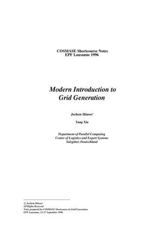
19. 10
craft as well as automobiles a reality. No longer are scientists and engineers restricted to wind
tunnel and free ßight experiments. On the numerical side, the development of high-speed comput-
ers as well as graphics workstations has allowed aerodynamicists to perform intricate calculations
that were unthinkable a few decades ago. A clear understanding of many of the aspects of subsonic
to hypersonic ßows, not attainable by wind tunnel experiments, is one of the important results of
these calculations. In addition, with the advent of massively parallel systems, a new era of CFD
(Computational Fluid Dynamics) has started, which will allow realistic simulations of turbulent
ßows with real gas effects (high temperature) past complex 3D conÞgurations. The purpose of
these notes is to present a clear, vivid, comprehensive treatment of modern numerical grid gener-
ation, based on boundary conforming grids, with emphasis on the actual grid generation process
as applied to complete geometries. Special emphasis is placed on algorithms and examples will be
presented along with a discussion of data structures and advanced programming techniques, topics
nearly almost always neglected in the scientiÞc and engineering Þeld. With the advent of modern
programming languages like C and C++, a revolution in scientiÞc programming is taking place.
Engineers, used to Fortran since the late Þfties, Þnally begin to realize that a new way of thinking
is needed in software engineering, characterized by the concept of object-oriented-programming.
Only with this approach it can be hoped to reduce the size and complexity of source code, to fully
use available hardware, to write and maintain very large software packages and to implement them
on arbitrary computer architectures. Grid generation packages like GridPro, and Grid code [20]
are based exclusively on C, X-Windows, and Open Gl, allowing full portability. Although nearly
two decades have past since the work of Thompson et al., the development of generally applicable
and easy to use 3D grid generation codes still presents a major challenge. In the case of structured
grids it was soon recognized that branch cuts and slits or slabs did not offer sufÞcient geometrical
ßexibility. Therefore, the majority of structured grid generation codes now employs the multiblock
concept, which is unstructured on the block level but results in a structured grid within a block.
To determine the block topology of a complex SD (solution domain) requires a certain effort. The
recent AZ–manager code (see Sec.??) is a major step forward in automatic topology deÞnition.
Grid generation has to embedded in the overall solution process that is depicted in Fig. 3.1.
Most important are tools for data conversion to directly use CAD data and to automatically inter-
face a grid to the ßow solver.
In the chart of Fig.3.1 the complete modelization process to obtain a ßow solution is shown. It
is assumed that a surface description of the vehicle is available, generally coming from the design
ofÞce in a CAD format, e.g. CATIA. This information has to be processed to convert it into a
format that can be read by the modules of Grid . Various conversion modules are available. The
chart then shows the grid generation process, where each module generates output that can be read
by the following modules, producing some kind of pipeline. The interfacing to the ßow solver
is done automatically and results can be visualized directly by the Plot3D package from NASA
Ames or by any other package that supports this format, e.g. the widely known Tecplot software
from AMTEC Engineering.
In practice, problems may be encountered with the grid generated and the ßow solution may
not be obtained, either because there is no convergence of the ßow solution, or after a few iterations
the solution may blow up. This depends very much on the ßow physics and to a large extent on
the experience of the user. These codes do not yet have reached a stage where they can be used as
a black box. A case with Ma of 25 and thermo-chemical nonequilibrium Navier-Stokes equations
is of course much harder to solve than an Euler problem at Ma 2. The stiffness of the equations

20. Numerical Grid Generation 11
PAW-Diagram
Parallel Aerodynamics Workbench
surface/grid
visualization
modification
triangular grid
surface plot3d
plot3d
mbview
NASA CFD−
standard
CAD−data
Tripla GridPro
IGES Halis PDC Halis p3d2cmd
PDC−CLE
TIL
code
topology TIL code wireframe
builder file
cmd
wireframe file
visualization
modification
Visual3 flow ParNSS
MIT solution PDC−CLE
project
file
Figure 3.1: In this chart the complete modelization process starting from the surface description
of the vehicle, coming from the design ofÞce, to the visualized results of a 3D ßow solution is
depicted. The necessary data Þles along with the corresponding software modules are shown.

21. 12
depends on the physics and also on the grid. A Navier-Stokes grid for a 3D vehicle with a cell
aspect ratio of 106 in the boundary layer is not only much more difÞcult to generate but it is also
much harder for the numerical scheme to converge to the physical solution in an efÞcient way.
Although the emphasis of these lecture notes is on grid generation, some results for Euler and N-S
calculations are presented.

22. Numerical Grid Generation 13
3.0.3 What Is a Good Grid
First, the discussion will be restricted to multi–block grids. It is felt that any kind of geometry can
be gridded by this approach, resulting in a superior grid quality when compared with unstructured
grids, in particular for viscous ßows. However, it should be kept in mind that grids of tens of thou-
sands of blocks have to be generated (automatically). On the block level the grid is completely
unstructured. The large number of blocks is needed because of complex topology, for instance,
there may be hundreds of bodies in the ßowÞeld, or, because the solver is run on a MIMD (Mul-
tiple Instruction Multiple Data) massively parallel system that may comprise several thousand
processors.
Second, the answer is straightforward, namely that it is not possible to deciding by simply
looking at a grid whether it is good or not. However, there exist several criteria that tell when
grid quality is not good.
º high degree of skewness
º abrupt changes in grid spacing
º insufÞcient grid line continuity (C0 , C1 , or C2 )
º nonalignment of the grid with the ßow
º insufÞcient resolution to resolve proper physical length scales
º grid topology not well suited to sufÞciently cover the ßow physics
º grid lacks special features needed by physical submodels
º grid is not singularity free (e.g. at stagnation point)
The Þrst three points are mostly independent of the ßow physics. Their effect is that they
reduce the order of the numerical scheme, and hence the accuracy of the results may deteriorate.
However, the magnitude of these effects will depend on the underlying ßow physics.
The other topics are strongly coupled with the ßow physics. It is known from numerical error
investigations that locally 1D ßow (proper grid alignmnet) will give an improved numerical accu-
racy, e.g. grid lines conforming to the boundary of a body will produce better accuracy. Length
scales have to be properly resolved (e.g. boundary layer), otherwise the physics cannot be ade-
quately represented, resulting in, for example, the wrong drag or skin friction. Grid topology also
has an inßuence on the physical results. An O-type topology for a 4 element airfoil may be ade-
quate for Euler solutions, but may be insufÞcient to resolve the wake resulting from viscous ßow,
necessitating a C-H type topology. Physical submodels may, for example, need grid line orthogo-
nality at Þxed boundaries. This is the case for some turbulence models to determine the distance
from the wall. Grids having a singularity, e.g. at the nose part of an aircraft, may lead to substan-
tially increased computing time because of a slowdown in convergence, since no information can
cross the singularity.

23. 14
3.0.4 Aspects of Multiblock Grid Generation
Structured grids use general curvilinear coordinates to produce a body Þtted mesh. This has the
advantage that boundaries can be exactly described and hence BCs can be accurately modeled.
In early grid generation it was attempted to always map the physical solution domain (SD) to a
single rectangle or a single box in the computational domain (CD). For multiply connected SDs,
branch cuts had to be introduced, a procedure well known in complex function theory and analytic
mapping of 2D domains, e.g. the Joukowski airfoil proÞle. However, it became soon obvious
that certain grid line conÞgurations could not be obtained. If one considers for example the 2D
ßow past an inÞnitely long cylinder, with a small enough Re number, it would be advantageous
if the grid line distribution would be similar to the streamline pattern. A 2D grid around a circle
which is mapped on a single rectangle necessarily has O-type topology, unless additional slits
(double valued line or surface) or slabs (blocks are cut out of the SD) are introduced. The main
advantage of the structured approach, namely that one only has to deal with a rectangle or a box,
that is a code is needing only 2 or 3 ”for” loops (C language), has been lost. The conclusion is
that this amount of structuredness is too rigid, and some degree of unstructuredness has to be
introduced. From differential geometry the concept of an atlas consisting of a number of charts is
known. The set of charts covers the atlas where charts may be overlapping. Each chart is mapped
onto a single rectangle. In addition, now the connectivity of the charts has to be determined. This
directly leads to the multiblock concept, which provides the necessary geometrical ßexibility and
the computational efÞciency for the Þnite volume or Þnite difference techniques.
For a vehicle like the Space Shuttle a variety of grids can be constructed (see Sec. ??). One
can start with a simple monoblock grid that wraps around the vehicle in an O-type fashion. This
always leads to a singular line, which normally occurs in the nose region. This line needs special
treatment in the ßow solution. It has been observed that convergence rate is reduced, although
special numerical schemes have been devised to alleviate this problem. Furthermore, a singularity
invariably leads to a clustering of grid points in an area where they are not needed. Hence, com-
puting time may be increased substantially. In addition, with a monoblock mesh gridline topol-
ogy is Þxed. Additional requirements with regard to grid uniformity and orthogonality cannot be
matched. The fourblock grid shown in Sec. ?? removes the singularity but otherwise retains the O-
type structure. The number of gridpoints is reduced substantially. The grid is smooth across block
boundaries. Therefore, no special discretization in the ßow solver across boundaries is needed. A
94 block Euler grid for the Shuttle has been generated, which includes the body ßap. The larger
number of blocks is needed to get a special grid line topology, and to better represent the ßow
physics (see discussion in Sec.??).
Since multiblock grids are unstructured on the block level, information about block connec-
tivity is needed along with the of each block. For reasons of geometrical ßexibility it is mandatory
that each block has its own local coordinate system. Hence blocks can be rotated with respect to
each other (Sec. 3.2.3). Slope continuity across neighboring block boundaries is achieved by over-
lapping edges (2D) or faces (3D). For grid generation an overlap of exactly 1 row or 1 column is
needed (2D). The ßow solver ParNSS needs an overlap of 2 faces.
The solution domain is subdivided into a set of blocks or segments (in the following the words
block and segment are used interchangeably). The overlap feature facilitates the construction of
the ßow solver substantially and allows the direct parallelization of the code on massively parallel

24. Numerical Grid Generation 15
systems using message passing.
Each (curvilinear) block in the physical plane is mapped onto a Cartesian block in the com-
putational plane (CP). The actual solution domain on which the governing physical equations are
solved is therefore a set of connected, regular blocks in the computational plane. However, this
does not mean that the solution domain in the computational plane has a regular structure, rather
it may look fairly fragmented. For the parallelization the important point is that there is no near-
est neighbor relation for the blocks. Therefore communication among blocks follows an irregular
pattern. A parallel architecture that is based on nearest neighbor communication, e.g. lattice gauge
theory problems, will not perform well for complex aerodynamic applications, simply because of
the communication overhead, caused by random communication.
The grid point distribution within each block is generated by the solution of a set of three
Poisson equations, one for each coordinate direction. The right hand side of the Poisson equations
is used for grid point control and is determined from the speciÞed grid point distribution on the
surfaces. That means that Þrst the right hand side is determined for each grid point on a surface and
then the values of the control functions are interpolated into the interior of the solution domain,
with some additional smoothing. In this context a grid point is denoted as boundary point if it
lies on one of the six faces of a block in the CP. However, one has to discern between physical
boundary points on Þxed surfaces that can be used for computation of the right hand side of
the Poisson equation and matching boundary points on overlap surfaces connecting neighboring
blocks. The positions of the latter ones are not known a priori but are determined in the solution
process (see above). All grid point positions on the faces of a block must be known before the
Poisson equations for this block can be solved to determine the grid point positions of the interior
points.
A coordinate transformation of the governing physical equations and their respective boundary
conditions from the physical plane to the computational plane is also required.

25. 16
3.1 Equations of Numerical Grid Generation
3.1.1 Elliptic Equations for 2D Grid Generation
In the following the elliptic PDEs used in the grid generation process will be derived, using the
mathematical tools of the previous section. First, we wish to explain the motives leading to this
approach. In the past, Þnite differences and Þnite elements have been used extensively to solve
computational problems. The latter have been mainly used in structural mechanics. About two
decades ago, Thompson et al.( see e.g. [2]) introduced the concept of a boundary Þtted grid (BFG)
or structureg grid (SG), that is a grid whose grid lines are aligned with the contours of the body.
Clearly, such a grid has to have coordinate lines, i.e. it cannot be completely unstructured. In
computational ßuid dynamics (CFD) in general and in high speed ßows in particular many ßow
situations are encountered where the ßow in the vicinity of the body is aligned with the surface, i.e.
there is a prevailing ßow direction. This is especially true in the case of hypersonic ßow because
of the high kinetic energy. The use of a SG, allows the alignment of the grid in that direction,
resulting in locally quasi 1D ßow. Hence, numerical diffusion can be reduced, i.e. better accuracy is
achieved. A BFG exactly matches curved boundaries, and for complex SDs generally will consist
by a set of so called blocks, which are connected. In the approach taken by the authors, a SD may
be covered by a set of hundreds or even thousands of blocks. Second, SGs can be made orthogonal
at boundaries, facilitating the implementation of BCs (Boundary Condition) and also increasing
the numerical accuracy at boundaries. Furthermore, orthogonality will increase the accuracy when
algebraic turbulence models are employed. In the solution of the N-S (Navier-Stokes) equations,
the BL (Boundary Layer) must be resolved. This demands that the grid is closely wrapped around
the body to describe the physics of the BL (some 32 layers are used in general for SGs or UGs).
Here some type of SG is indispensable. In addition, to describe the surface of the body a structured
approach is better suited.
The resolution of the BL leads to large anisotropies in the length scales in the directions along
and off the body. Since the time-step size in an explicit scheme is governed by the smallest length
scale or, in the case of chemical reacting ßow, by the magnitude of the chemical production terms,
extremely small time steps will be necessary. This behavior is not demanded by accuracy but to
retain the stability of the scheme. Thus, implicit schemes will be of advantage. In order to invert the
implicit operator, factorization is generally used, resulting in two factors if LU decomposition (that
is, factoring in the direction of the plus and minus eigenvalues of the Jacobians) is employed, or in
three factors if the coordinate directions are used. For the unstructured approach there is no direct
way to perform this type of factorization. Moreover, the use of the so-called thin layer approach,
that is retaining the viscous terms only in the direction off the body, reduces the computer time by
about 30 %. Since there are no coordinate lines in the UG, this simpliÞcation is not possible. A
fairly complex procedure would be needed to artiÞcially construct these lines. Moreover, the ßow
solver based on the UG is substantially slower than for the SG. This is due to the more complicated
data structure needed for UGs. Factors of 3, and by some authors of up to 10, have been given in
the literature.
In order to calculate heat loads for vehicles ßying below Ma 8, turbulence models have to
be used, for example, the difference in surface temperature for S¨ nger at cruising speed (around
a
Ma 5) is about 500 K depending on laminar or turbulent ßow calculations. Depending on the real

26. Numerical Grid Generation 17
surface temperature encountered in ßight a totally different type of vehicle has to be designed
since a cooled Titanium wall cannot withstand a temperature of 1300 K for a long period (about
20 minutes). Therefore turbulent calculations are of high importance. Only a SG can provide the
alignment along with the orthogonality at the boundary to accurately perform these calculations.
In general, SG provide sophisticated means both for clustering and adaptation using redistri-
bution or local enrichment techniques. A comparison of these two approaches is given by Dannen-
hoffer [2] where local enrichment gives somewhat better results. However, it is much more costly
to use. In many cases of practical interest, for example Þne resolution of a bow shock or a canopy
shock and in situations where shocks are reßected, the alignment of the grid can result in a more
accurate solution than randomly Þlling the space with an enormously large number of smaller and
smaller tetrahedrons or hexahedrons.
The highest degree of freedom of course is obtained in UGs. The majority of physical phe-
nomena encountered in external and also in internal ßows exhibit certain well ordered structures,
such as a bow shock or system of reßected shocks or some type of shock-shock interaction, which
can be perfectly matched by adaptive grid alignment, coupled to the solution process.It is therefore
felt, however, that mesh redistribution and alignment is totally adequate for the major part of the
ßow situations encountered in CFD, especially in aerodynamics.
Only if a very complex wave pattern evolves due to special physical phenomena, for example,
generating dozens of shock waves coming from an explosion, the UG seems to be advantageous.
In addition, the coupling of SGs with UGs is possible as has been shown by Weatherill and
Shaw et al. [40]. Such a grid is called a hybrid grid.
A mixture between the boundary Þtted grid approach and the completely unstructured ap-
proach is the use of multiblock grids, which has been employed in the Grid [27] and in the
GridPro[35] packages. On the block level the grid is unstructured, that is the blocks itself can
be considered as Þnite elements, but within each block the grid is structured and slope continuity
is provided across block boundaries (on the coarsest level). If a block is reÞned locally, this fea-
ture cannot be maintained. Recently a 94 block grid (Euler) and a 147 block grid (N-S) for the
Space Shuttle have been generated, demonstrating the variability of this approach. Moreover, the
automatic zoning feature of GridProhas been used to generate a grid of several thousand blocks
(see Sec. ??).
For the derivation of the transformed grid generation equations one starts from the original
Poisson equations and then the role of the dependent and independent variables is interchanged.
∆ξ P; ∆η Q (3.1)
Using (2.34), the transformation equation of the Laplacian, and the fact that ξ and η are coor-
dinates themselves, we Þnd
∆ξ gik ´ξ i k Γik ξ
j
j µ gik ei k ¡ e1 (3.2)

27. 18
1
∆ξ Ô yη ´g11 xξξ · 2g12 xξη · g22 xηη µ xη ´g11 yξξ · 2g12 yξη · g22 yηη µ P (3.3)
g
In a similar way we obtain for the η coordinate
∆η
·1
Ô yξ ´g11 xξξ · 2g12 xξη · g22 xηη µ xξ ´g11 yξξ · 2g12 yξη · g22 yηη µ Q (3.4)
g
By means of (2.37), the gi j can be expressed in terms of gi j . For stability reasons in the nu-
merical iterative solution of the above system of equations, the above equations are rewritten in
the form
g22 xξξ 2g12 xξη · g11 xηη · g´xξ P · xη Qµ 0
g22 yξξ 2g12 yξη · g11 yηη · g´yξ P · yη Qµ
(3.5)
0
These equations are quasilinear, where the non-linearity appears in the expression for the met-
ric coefÞcients.
For 2D, using the original functions P and Q and coordinates x, y and ξ, η, one obtains:
g22 xξξ 2g12 xξη · g11 xηη · g´xξ P · xη Qµ 0
g22 yξξ 2g12 yξη · g11 yηη · g´yξ P · yη Qµ
(3.6)
0
where
g11 x2 · y2
ξ ξ g12 g21 xξ xη · yξ yη g22 x2 · y2
η η
g11 g22 g g12 g21 gg12 gg21 g22 gg11 (3.7)
g ´xξ yη xξ yη µ2
is used. The numerical solution of Eqs.(3.6) along with speciÞed control functions P, Q as
well as proper BCs is straightforward, and a large number of schemes is available. Here a very
simple approach is taken, namely the solution by Successive-Over-Relaxation (SOR). The second
derivatives are described in the form
´xξξ µi j xi·1 j 2xi j · xi 1 j
´xηη µi j xi j·1 2xi j · xi j 1 (3.8)
´xξη µi j 1 4´xi·1 j·1 xi 1 j·1 xi·1 j 1 · xi 1 j 1µ
Solving the Þrst of Eqs.(3.6) for xi j yields the following scheme

28. Numerical Grid Generation 19
xi j 1 2´αi j · γi j µ 1 αi j ´xi·1 j xi 1 j µ
βi j ´xi·1 j·1 xi 1 j·1 xi·1 j 1 · xi 1 j 1µ·
γi j ´xi j·1 xi j 1 µ· (3.9)
1 2Ji2 j Pi j ´xi·1 j xi 1 j µ·
Ó
1 2Ji2 j Qi j ´xi j·1 xi j 1 µ
where the notation J2 g, αi j g22 , 2βi j g12 , and γi j g11 was used. Overrelaxation is
achieved by computing the new values from
xnew xold · ω´x xold µ 1 ω 2 (3.10)
The solution process for a multiblock grid is achieved by updating the boundaries of each
block, i.e. by receiving the proper data from neighboring blocks and by sending overlapping data
to neighboring blocks. Then one iteration step is performed using these boundary data, iterating on
all interior points. After that, those newly iterated points which are part of the overlap are used to
update the boundary points of neighboring blocks and the whole cycle starts again, until a certain
number of iterations has been performed or until the change in the solution of two successive
iterations is smaller than a speciÞed bound.
3.1.2 Elliptic Equations for Surface Grid Generation
x
A curved surface can be deÞned by the triple y ´u vµ,
z
where u and v parametrize the surface. DeÞning a new coordinate system on such a surface only
means another way of parametrization of the surface, i.e. a transformation from ´u vµ to ´ξ ηµ,
which is a mapping from R2 R3 . To obtain the new coordinates Poisson equations are used. The
derivation for the surface grid generation equations is similar as in the 2D or 3D case. Using the ∇
operator of equation 2.18, the surface grid generation equations take the form
j
∆ξ gik ξ i k Γik ξ j P
j
(3.11)
∆η gik η i k Γik η j Q
In this case the derivatives are with respect to u and v, and not with respect to ξ and η. There-
fore, the metric is given by the transformation of the parameter space ´u vµ to physical space
´x y zµ, i.e ei ∂i ´x y zµ with ∂1 ∂u and ∂2 ∂v . To obtain the familiar form of the equations,
i.e. ´u vµ values are the boundary points in the ´ξ ηµ grids in the computational plane (CP), the
dependent and independent variables in Eqs. 3.11 need to be interchanged. Introducing the matrix
M of the contravariant row vectors from the transformation ´u vµ ´ξ ηµ,
ξu ηu
M (3.12)
ξv ηv

29. 20
and the inverse matrix, M 1 , formed by the covariant columnvectors,
uξ uη
M 1 vξ vη (3.13)
along with the deÞnition of S : ´ξ ηµT the surface grid equations Eqs. 3.11 take the following
form:
gik Γ1 P
gik S i k M ik
Q (3.14)
gik Γ2
ik
From this folllows
gik ξ i k gik Γ1
M 1 M 1
P ik
Q (3.15)
gik η i k gik Γ2
ik
The surface metric induces, in comparison with the plain 2D case, additional terms that are
independent of ξ η and act as some kind of control functions for the grid line distribution. To
determine the Þnal form of the equations the role of the independent and the dependent variables
in the second derivatives ξ i k η i k have to be interchanged. This is done as follows. The matrix of
covariant row vectors M can be written in the form
ξu ξv 1 vη uη
M ηu ηv vη uξ (3.16)
J
Hence, ξuu ´ξu µu
v ¡η
where ∂u ξu ∂ξ · ηu ∂η . This results in the following second
J u
derivatives
1 Ò Ó
ξuu ξu v2 uξξ 2vξ vη uξη · v2 uηη ξv v2 vξξ 2vξ vη vξη · v2 vηη
η ξ η ξ (3.17)
J2
1
ξu u2 uξξ 2uξ uη uξη · u2 uηη
ξvv J2 η ξ Ó (3.18)
ξv u2 vξξ 2uξ uη vξη · u2 vηη µ
η ξ
¡
ξu uη vη uξξ uη vξ · vη uξ uξη · uξ vξ uηη
¡
ξuv 1
J2 ¡
ξv uη vη vξξ uη vξ · vη uξ vξη · uξ vξ vηη
¡· (3.19)
ηuu 1
J2
ηu v2 uξξ 2vξ vη uξη · v2 uηη
η ξ
(3.20)
ηv v2 vξξ 2vξ vη vξη · v2 vηη
η ξ

30. Numerical Grid Generation 21
The quantities ηvv and ηuv are transformed similar. With the deÞnition of S stated above the
formulas can be summarized as:
1 v2 uξξ 2vξ vη uξη · v2 uηη
η ξ 1
Suu M : Ma (3.21)
J2 v2 vξξ 2vξ vη vξη · v2 vηη
η ξ J2
¡
uη vη uξξ uη vξ · vη uξ uξη · uξ vξ uηη
Suv
1
M ¡
uη vη vξξ uη vξ · vη uξ vξη · uξ vξ vηη
:
1
Mb (3.22)
J2 J2
1 u2 uξξ 2uξ uη uξη · u2 uηη 1
M´ 2 µ
η ξ
Svv : Mc (3.23)
J2 uη vξξ 2uξ uη vξη · u2 vηη
ξ J2
Sustituting the above formulas for S i j into Eq. 3.15 yields
1 11
g a · 2g12 b · g22 c
¡ · M 1 P
gik Γ1
ik (3.24)
J2 Q gik Γ2
ik
Sorting the vectors a b c with respect to the second derivatives of r ´u vµ, then one obtains
1
αrξξ 2βrξη · γrηη
¡ · M 1 P
gik Γ1
ik (3.25)
J2 Q gik Γ2
ik
where
α g11 v2 2g12 uη vη · g22 u2
η η
β g11 vξ vη g12 ´uξ vη · vξ uη µ· g22 uξ uη (3.26)
γ g11 v2 2g12 uξ vξ · g22 u2
ξ ξ
M 1 has been deÞned previously. In the numerical solution of Eq. 3.26 that uses simple SOR,
only terms rξξ and rηη contain values ui j and vi j for which the surface equations have to be solved
for. One has to note that the metric is also a function of variables u v. In the case of planes the
equations reduce to the well known 2-dimensional grid generation equations.
For the numerical calculation of the surface Christoffel symbols the following formulas are
used. Given a function f ´u vµ, derivatives fu , fv , fuv , fuu and fvv are needed. For surfaces in 3D
space one has
e1 ´xu yu zv µ
e2 ´xv yv zv µ (3.27)

31. 22
The numerical procedure for the calculation of the metric is as follows. First, all derivatives
xu xv xuu xuv xvv etc. have to be calculated. After that, the 5 quantities gi j and gi j Γ1j have to be
i
stored at each grid point. These quantities and not the coordinate values ´x y zµ should be interpo-
lated in the generation of the surface grid.
Using the relations of Sec. 2.0
g11 x2 · y2 · z2
xu xv · yu yv · zu zv
u u u
g12 (3.28)
g22 x2 · y2 · z2
v v v
the determinant of the metric tensor is
g g11 g22 g2
12 (3.29)
and the contravariant metric coefÞcients are :
g11 g22 g
g12 g12 g (3.30)
g22 g11 g
From this the Christoffel symbols can be determined.
Γ1 e1 ¡ ei k
ik (3.31)
Γ2
ik e2 ¡ ei k
e1 g1k ek g11 e1 · g12 e2 ´·g22e1 g12e2 µ g
(3.32)
e2 g2k ek g21 e1 · g22 e2 ´ g12e1 · g11e2 µ g
Γ1
11 e1 ¡ e1 1 e1 xuu · e1 yuu · e1 zuu
x y z
Γ1
12 e1 ¡ e1 2 e1 xuv · e1 yuv · e1 zuv
x y z (3.33)
Γ1
22 e1 ¡ e2 2 e1 xvv · e1 yvv · e1 zvv
x y z
Resulting in
e1 g11 xuu · 2g12 xuv · g22 xvv
¡·
gi j Γ1j
i x
e1 g11 yuu · 2g12 yuv · g22 yvv
¡·
y
e1 g11 zuu · 2g12 zuv · g22 zvv
¡ (3.34)
z
An analog result follows for gi j Γ2j . All terms have a common factor 1 g.
i

32. Numerical Grid Generation 23
3.1.3 Elliptic Equations for 3D Grid Generation
The following general coordinate transformation from the cartesian coordinate system, denoted
by coordinates ´x y zµ, to the CD, denoted by coordinates (ξ, η, ζ), is considered. The one to one
transformation is given by (except for a Þnite (small) number of singularities):
x x´ξ η ζµ; ξ ξ´x y zµ
y y´ξ η ζµ; η η´x y zµ (3.35)
z z´ξ η ζµ; ζ ζ´x y zµ
Since there is a one-to-one correspondence between grid points of the SD and CD (except for
singular points or singular lines), indices i, j, and k can be used to indicate the grid point position.
The grid in the CP is uniform with grid spacings ∆ξ = ∆η = ∆ζ = 1. Similar as in 2D, a set of
Poisson equations is used to determine the positions of (ξi , η j , ζk ) in the SD as functions of x y z.
In addition, proper Boundary Conditions (BC) have to be speciÞed. Normally, Dirichlet BCs are
used, prescribing the points on the surface, but for adaptation purposes von Neumann BCs are
sometimes used, allowing the points to move on the surface, in order to produce an orthogonal
grid in the Þrst layer of grid points off the surface. The Poisson equations for the grid generation
read:
ξxx · ξyy · ξzz P
ηxx · ηyy · ηzz Q (3.36)
ζxx · ζyy · ζzz R
where P Q R are so-called control functions that depend on ξ, η and ζ.
However, this set of equations is not solved on the complex SD, instead it is transformed to the
CD. The elliptic type of Eqs.(3.36) is not altered, but since ξ, η and ζ are coordinates themselves,
the equations become nonlinear. In more compact notation the elliptic generation equations read.
∆ξ P; ∆η Q; ∆ζ R (3.37)
where planes of constant ξ, η or ζ form the boundaries and x, y, z are now the dependent
variables. Equations 3.37 are solved in the computational plane using Eq.2.18. The x, y, z coor-
dinate values describing the surfaces which form the boundary of the physical solution domain,
are now used as boundary conditions to solve the transformed equations below. To perform the
transformation the ∆-operator in general curvilinear coordinates is used:
j
∆Ψ gik Ψ i k Γik Ψ j (3.38)
where Ψ is a scalar function. The determinant of the metric tensor, g, is given by the
transformation from (x,y,z) to ´ξ η ζµ. The co -and contravariant base vectors are given by
ei ∂i ´x y zµ ; ei ∂i ´ξ η ζµ with ∂1 ∂ξ ∂1 ∂x etc.

33. 24
gi j ei ¡ e j ; Γijk ei ¡ e j k ´¡ denotes scalarproductµ (3.39)
If ξ, η or ζ is inserted for Ψ, the second derivatives are always zero and Ψ i 1 only for j=1
if variable ξ is considered etc. Eqs. 3.37 then become
gik Γ1
ik P ; gik Γ2
ik Q ; gik Γ3
ik R (3.40)
or in vector notation
¼ g11x · 2g12x · ½
ξξ ξη P
E ¡ g yξξ · 2g yξη ·
11 12 Q (3.41)
g11 zξξ · 2g12 zξη · R
¼ ½
e1
where E e2 is the matrix consisting of the contravariant row vectors. The inverse
e3
matrix is F ´e1 e2 e3 µ consisting of the covariant column vectors. Thus E 1 F and Þnally the
3d grid generations are in the form
¼ g11x · ½
ξξ P
g yξξ ·
22
F ¡ Q (3.42)
g33 zξξ · R