RNA Seq Data analysis

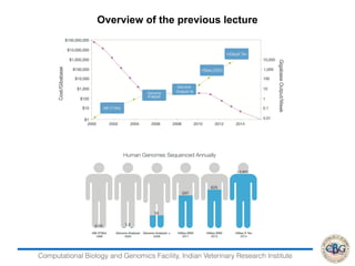
1. Computational Biology and Genomics Facility, Indian Veterinary Research Institute
Overview of the previous lecture

2. Computational Biology and Genomics Facility, Indian Veterinary Research Institute
Overview of the previous lecture

3. Computational Biology and Genomics Facility, Indian Veterinary Research Institute
Instrument
Needed
Coverage
Throughput/
Run
Human
Genome/run
Cost per Run** Total Cost $/Genome
HiSeq 2500 30x 1Tb 11 29.000 29,000 2,536
HiSeq x 10 30x 1 STb 16 15.700 12,000 950
Pacbio RSII 54x 1 Gb 0.000 212 34,374 34,374
PacBio Sequel 50x 5-10 Gb 0.06 700 10,300 10,500
Current Loading Technologies
Platform Average Reeds
length
Advantages Limitation
Material
Recommended
Illumina MiSeq 2 x 300 bps Accurate Short Length 100-200 ng
Illumina Mole-
culo
5 Kbps Accurate Coverage may
Fluctuate
10 ug
Pacific
Bioscience
15 Kbps Long reads Relatively
expensive
10-100 ug
Oxford
Nanopore
5 Kbps Low ownership
cost
High error rate 1 ug
Long-Range Sequencers Comparison

4. Computational Biology and Genomics Facility, Indian Veterinary Research Institute
Basics of RNA - seq data analysis

5. Computational Biology and Genomics Facility, Indian Veterinary Research Institute
• Sequence DNA
• De novo sequencing
• Reference based re-sequencing - SNP, CNV and indels
• Metagenomics - Identify who is there in a mixture of microbes
• Sequence RNA
• RNA-Seq (Transcriptome wide sequencing)
• miRNA - Seq novo sequencing
• Novel NcRNAs
• Study Protein-DNA/RNA interactions
• ChIP-Seq (TFs)
• CLIP - Seq (For RNA binding proteins)
• Epigenetics
• DNA methylation
• Histone modification (ChIP-seq)
• Nucleosome positioning
• Chromosome looping
Applications of NGS

6. Computational Biology and Genomics Facility, Indian Veterinary Research Institute
Certain important key words to be remembered
from the previous chapter
• Sequencing
• both DNA and RNA (with modified protocol)
• Short reads
• 35, 50, 75, and 100-bp (Solexa and SOLiD)
• 400-bp (454)
• Ultra-high throughput
• 1 to 1.5 billion reads (Solexa and SOLiD)
• 2- 4 million reads (454)

7. Computational Biology and Genomics Facility, Indian Veterinary Research Institute
• The transcriptome : Complete set of transcripts in a cell, both in terms
of type and quantity.
• Transcriptome analysis -
• in understanding the pattern of gene expression to address basic
biological questions.
• greater insights into biological pathways and molecular mechanisms
that regulate cell fate, development, and disease progression.
What is a transcriptome?
Transcriptome can be studied through RNA-seq/microarray

8. Computational Biology and Genomics Facility, Indian Veterinary Research Institute
RNA sequencing

9. Computational Biology and Genomics Facility, Indian Veterinary Research Institute
Aim of RNA-seq experiment
• To quantify RNA abundance
• To determine the transcriptional structure
of genes: start sites, 5’ and 3’ ends,
splicing patterns
• To quantify the changing expression levels
of each transcript during development and
under different conditions
• To identify variants on the transcripts

10. Computational Biology and Genomics Facility, Indian Veterinary Research Institute
Basic work flow of Next generation sequencing
Wang et al., 2009

11. Computational Biology and Genomics Facility, Indian Veterinary Research Institute
What can we get out of RNA-seq experiment?
Gene expression
Alternative splicing
Transcript variation
Non-coding RNAs
RNA -seq
Different expression
Non- syn SNPs
Synonymous SNPs
SNPs in 3’- UTRs
Allele specific
expression
Protein changes
RNA binding proteins
microRNA binding
sites

12. Computational Biology and Genomics Facility, Indian Veterinary Research Institute
Microarray
Normal RNA
Cy3 Labelling
Reverse transcription
Experimental RNA
Cy5 labelling
Hybridize Wash & Scan

13. Computational Biology and Genomics Facility, Indian Veterinary Research Institute
RNA - Seq vs Microarray
“RNA- seq…. is expected to revolutionise the manner in
which eukaryotic transcriptome are analysed”
Wang et al. Nat Rev Gen, 2009

14. Computational Biology and Genomics Facility, Indian Veterinary Research Institute
Limitations of microarray platforms
• High background levels owing to cross-hybridization;
• Limited dynamic range of detection owing to both background and
saturation of signals.
• Reliance upon existing knowledge about genome sequence;

15. Computational Biology and Genomics Facility, Indian Veterinary Research Institute
RNA - seq has higher dynamic range
For microarrays:
• Low signal end: high background noise
• High signal end: signals will be saturated
With proper depth, NGS can solve this problem well

16. Computational Biology and Genomics Facility, Indian Veterinary Research Institute
Comparison of Microarray with RNA - seq

17. Computational Biology and Genomics Facility, Indian Veterinary Research Institute
Experimental considerations

18. Computational Biology and Genomics Facility, Indian Veterinary Research Institute
Sample preparation
• Amount requirement
• 100 ug total RNA (several Wold’s studies)
• 2 ug total RNA (Center for Medical Genomics, SOLiD)
• 50 ng total RNA (collaboration with Pourmand, SOLiD)
• Single cell (Tang et al. Nat. Methods, 2009)
(when RNA is limiting, approaches to amplify small quantities of RNA exist)
• rRNA removal
• rRNAs are highly abundant (>90% of total RNA)
Solutions:
• rRNA depletion kits
• Poly-A selection
• Using enzymes that selectively degrade uncapped RNA

19. Computational Biology and Genomics Facility, Indian Veterinary Research Institute
Sample preparation
• Reverse transcription (RNA -> cDNA)
• oligo dT
• Pros: Focusing on polyA ed transcriptions cleaner.
• Cons: Bias towards the 3’-end of transcripts
• Random primers
• Pros: Equal coverage, can be used to study non-polyAed transcripts
• Cons: higher proportion of rRNA

20. Computational Biology and Genomics Facility, Indian Veterinary Research Institute
Single end reads vs paired ends reads
3' 5'
5' 3'
5'
3'
5' 3'
AAAA
AAAA
3' 5'TTTT
cDNA fragments and adapter ligation
cDNA conversion
R1
R2
5' 3'
3' 5'
Sequencing of each fragment
R1 will run in the same direction of the reference
R2 will run in the opposite direction of the reference

21. Computational Biology and Genomics Facility, Indian Veterinary Research Institute
Statistical considerations
Number of conditions?
• Dynamics?
• Dose-effect?
• Tissue-specificity?
Number of replicates?
Depth of sequencing?
• Biological variation, …
• Statistical power, …
• Gene expression
• Alternative splicing
• Allele specific expression
₹

22. Computational Biology and Genomics Facility, Indian Veterinary Research Institute
Basics of RNA - seq data analysis - II
Data processing

23. Computational Biology and Genomics Facility, Indian Veterinary Research Institute
Data analysis workflow
Primary analysis Tertiary analysis
• Image acquisition /
semiconductor based detection
• Base calling and
• Quality metrics
Secondary analysis
• Sequence alignment
• Sequence Stats
• Consensus Calling
• Sequence assembly
• Application specific analysis
• DNA-Seq
• Re-Sequencing
• De-novo Sequencing
• ChiP Sequencing
• RNA-Seq
• Epigenetics
Data analysis workflow

24. Computational Biology and Genomics Facility, Indian Veterinary Research Institute
Sequence alignment

25. Computational Biology and Genomics Facility, Indian Veterinary Research Institute
Sequence alignment
▪ Sequence alignment is a way of arranging the sequences of DNA, RNA,
or protein to identify regions of similarity
▪ Aligned sequences of nucleotide or amino acid residues are typically
represented as rows within a matrix.
▪ Gaps are inserted between the residues so that identical or similar
characters are aligned in successive columns.
1. To find whether two (or more) genes or proteins are evolutionarily
related to each other
2. To observe patterns of conservation (or variability).
3. To find structurally or functionally similar regions within proteins i.e to
find the common motifs present in both sequences.
4. To find out which sequences from the database are similar to the
sequence at hand
Purpose of sequence alignment

26. Computational Biology and Genomics Facility, Indian Veterinary Research Institute
1. They are often used interchangeably, they have quite different
meanings.
2. Sequence identity refers to the occurrence of exactly the same
nucleotide or amino acid in the same position in aligned sequences.
3. The term ‘sequence homology’ is the most important (and the most
abused) of the three.
• When we say that sequence A has high homology to sequence B,
then we are making two distinct claims:
• not only are we saying that sequences A and B look much the
same, but also that all of their ancestors also looked the same,
going all the way back to a common ancestor.
Identity vs Similarity vs Homology

27. Computational Biology and Genomics Facility, Indian Veterinary Research Institute
Sequence Identity Sequence similarity
Sequence
homology
Definition
Proportion of identical
residues between two
sequences.
Proportion of similar
residues between two
sequences. Two residues are
similar if their substitution cost
is higher than 0.
Sequences
derived from a
common
ancestor
Expressed as % identity % Similarity Yes or No
Rule-of-thumb: If two sequences are more than 100 amino acids long
(or 100 nucleotides long) they are considered homologues if 25% of the
amino acids are identical (70% of nucleotide for DNA).
Twilight zone = protein sequence similarity between ~0-20%

28. Computational Biology and Genomics Facility, Indian Veterinary Research Institute
Global alignment
• assumes that the two sequences are basically similar over the entire
length of one another.
• forces to match the sequences from end to end, even though parts of the
alignment are not very convincingly matching.
• most suitable when the two sequences are of similar length and are with a
significant degree of similarity throughout.
.
Computational approaches
• Global alignment
• Local alignment

29. Computational Biology and Genomics Facility, Indian Veterinary Research Institute
Local alignment
• Identifies segments of the two sequences that match well with no
attempt to force the entire sequences into alignment
• Parts that appear to have good similarity, according to some criterion
are aligned.
• Suitable when comparing substantially different sequences, which
possibly differ significantly in length, and have only short patches of
similarity

30. Computational Biology and Genomics Facility, Indian Veterinary Research Institute
Give two sequences we need a number to associate with each possible
alignment (i.e. the alignment score = goodness of alignment).
The scoring scheme is a set of rules which assigns the alignment
score to any given alignment of two sequences.
• The scoring scheme is residue based: it consists of residue substitution
scores (i.e. score for each possible residue alignment), plus penalties for
gaps.
• The alignment score is the sum of substitution scores and gap penalties.
Substitution scores are given by :
For DNA : Substitution Matrix for DNA (Purine/Purine or purine/pyramidine
substitutions)
For proteins : Substitution matrix based on Polarity, Size, Charge or
Hydrophobicity
Evolutionary distance matrices :- PAM and BLOSUM for
protein sequences

31. Computational Biology and Genomics Facility, Indian Veterinary Research Institute
Types of alignment
Pairwise alignment Multiple Sequence alignment
Can be Global or Local

32. Computational Biology and Genomics Facility, Indian Veterinary Research Institute
• Dot Matrix method
• The dynamic programming method
• Needleman and Wunch
• Smith and Watermann
• Heuristic methods - FASTA ; BLAST
Methods of pairwise alignment
• It is a visual graphical representation of similarities between two
sequences.
• Each axis represents one of the two sequences to be compared.
• In the dot matrix method when two sequences are similar over their entire
length a line will extend from one corner of the dot plot to the diagonally
opposite corner.
• If two sequences share only patches of similarity then it will be revealed
by diagonal stretches.
Dot Matrix method

33. Computational Biology and Genomics Facility, Indian Veterinary Research Institute
Interpretation of Dot Matrix
• Regions of similarity appear as diagonal runs of dots.
• Reverse diagonals (perpendicular to diagonal) indicate inversions.
• Reverse crossing diagonals (Xs) indicate palindromes.
Limitation:-
• The dot matrix computer programs do not show an actual alignment.

34. Computational Biology and Genomics Facility, Indian Veterinary Research Institute
The dynamic programming
• Dynamic programming reduces the massive number of possibilities that
need to be considered in aligning sequences.
• This method was first used for global alignment of sequences by
Needleman-Wunch algorithm (1970) and for local alignment by Smith -
Waterman algorithm (1981).
• Both the algorithms involve initialization, matrix filling (scoring) and trace
back steps. The algorithms use either PAM or BLOSUM matrices in the
scoring step to fill the score matrix.

35. Computational Biology and Genomics Facility, Indian Veterinary Research Institute
Global alignment

36. Computational Biology and Genomics Facility, Indian Veterinary Research Institute
The three main steps in this algorithm are :
1. Initialization
2. Matrix filling
3. Traceback for alignment
Initialization
1. Place the two sequences one across the row and other down the
column
2. The first column and first row should be a gap
3. Add the cumulative gap cost across the row and other down the
column to fill the first column and first row
Global alignment (Needleman and Wunch)

37. Computational Biology and Genomics Facility, Indian Veterinary Research Institute
• Matrix filling
• Rules :-
• Check the side, top and diagonal values of the box
• Box Beside - (add gap cost)
• Box top - ( add gap cost)
• Diagonal box - (match/mismatch)
• Put the highest value in the respective boxes
• Proceed to the end of the scoring matrix
• Trace back
• Start from the end of the matrix and reach the start by tracing back
the value obtained in the box
• if diagonal - Place the characters
• if vertical or horizontal - place a gap in the sequence being pointed
by the arrow

38. Computational Biology and Genomics Facility, Indian Veterinary Research Institute
gap T G A
gap 0 -2 -4 -6
A -2
-1 -4
-1
-4
-3 -6
-3
-3
-3 -8
-3
-5
T -4
-1 -3
-1
-6
-2 -5
-2
-3
-4 -5
-4
-4
G -6
-5 -3
-3
-8
0 -4
0
-5
-3 -6
-2
-2
C -8
-7 -5
-5
-10
-4 -2
-2
-7
-1 -4
-1
-4
Matrix Filling - Gap -2; Mismatch -1; Match +1 Box Beside : +gap; Box Top : +gap; Diagonal box : match or mismatch

39. Computational Biology and Genomics Facility, Indian Veterinary Research Institute
gap T G A
gap 0 -2 -4 -6
A -2
-1 -4
-1
-4
-3 -6
-3
-3
-3 -8
-3
-5
T -4
-1 -3
-1
-6
-2 -5
-2
-3
-4 -5
-4
-4
G -6
-5 -3
-3
-8
0 -4
0
-5
-3 -3
-2
-2
C -8
-7 -5
-5
-10
-4 -2
-2
-7
-1 -4
-1
-3
Trace back

40. Computational Biology and Genomics Facility, Indian Veterinary Research Institute
ATGC
- TGA
-2+1+1-1
= -1

41. Computational Biology and Genomics Facility, Indian Veterinary Research Institute
gap G A C T A C
gap 0 -1 -2 -3 -4 -5 -6
A -1
0 -2
0
-2
0 -3
0
-1
-2 -4
-1
-1
-3 -5
-2
-2
-3 -6
-3
-3
-5 -7
-4
-4
C -2
-1 -1
-1
-3
0 -1
0
-2
+1 -2
+1
-1
-1 -3
0
0
-2 -4
-1
-1
-3 -5
-2
-2
G -3
-1 -2
-1
-4
-1 -1
-1
-2
0 0
0
-2
+1 -1
+1
-1
0 -2
0
0
-1 -3
-1
-1
C -4
-3 -2
-2
-5
-1 -2
-1
-3
0 -1
0
-2
0 0
0
-1
+1 -1
+1
-1
+1 -2
+1
0
Matrix Filling - Gap -1; Mismatch - 0; Match +1

42. Computational Biology and Genomics Facility, Indian Veterinary Research Institute
Matrix Filling - Gap -1; Mismatch - 0; Match +1
gap G A C T A C
gap 0 -1 -2 -3 -4 -5 -6
A -1
0
-2
0
-2
0
-3
0
-1
-2
-4
-1
-1
-3
-5
-2
-2
-3
-6
-3
-3
-5
-7
-4
-4
C -2
-1
-1
-1
-3
0
-1
0
-2
+1
-2
+1
-1
-1
-3
0
0
-2
-4
-1
-1
-3
-5
-2
-2
G -3
-1
-2
-1
-4
-1
-1
-1
-2
0
0
0
-2
+1
-1
+1
-1
0
-2
0
0
-1 -3
-1
-1
C -4
-3
-2
-2
-5
-1
-2
-1
-3
0
-1
0
-2
0
0
0
-1
+1
-1
+1
-1
+1
-2
+1
0

43. Computational Biology and Genomics Facility, Indian Veterinary Research Institute
ACG-C
GACTAC
-1+1+1+0-1+1
= +1
AC-GC
GACTAC
-1+1+1-1+0+1
= +1

44. Computational Biology and Genomics Facility, Indian Veterinary Research Institute
gap T G A
gap 0 -2 -4 -6
A -2
T -4
G -6
C -8
Matrix Filling - Gap -2; Mismatch -1; Match +1 Box Beside : +gap; Box Bottom : +gap; Diagonal box : match or mismatch

45. Computational Biology and Genomics Facility, Indian Veterinary Research Institute
gap G A C T A C
gap 0
A -2
C -4
G -6
C -8
Matrix Filling - Gap -2; Mismatch - -1; Match +1

46. Computational Biology and Genomics Facility, Indian Veterinary Research Institute
gap G A C T A C
gap
A
C
G
C
Matrix Filling - Gap -1; Mismatch - 0; Match +1

47. Computational Biology and Genomics Facility, Indian Veterinary Research Institute
gap T G A
gap
A
T
G
C
Matrix Filling - Gap -2; Mismatch -1; Match +1 Box Beside : +gap; Box Bottom : +gap; Diagonal box : match or mismatch

48. Computational Biology and Genomics Facility, Indian Veterinary Research Institute
The three main steps in this algorithm are :
1. Initialization
2. Matrix filling
3. Traceback for alignment
Initialization
1. Place the two sequences one across the row and other down the
column
2. The first column and first row should be a gap
3. Place zeros in first column and first row
Matrix filling
1. The value of each box thereon depends on the top, diagonal and
side boxes (Box Beside - (add gap cost); Box top - ( add gap
cost); Diagonal box - (match/mismatch)
2. If the value is negative - put the value as zero
3. The highest of the three values is placed in the box
4. The same is continued till the end of the matrix
Smith and Waterman algorithm (Local alignment)

49. Computational Biology and Genomics Facility, Indian Veterinary Research Institute
gap T G A
gap 0 0 0 0
A 0
0 0
0
0
0 0
0
0
+1 0
+1
0
T 0
+1 0
+1
0
0 0
0
0
0 0
0
0
G 0
0 0
0
0
+2 0
+2
0
0 0
0
0
C 0
0 0
0
0
0 0
0
0
+1 0
+1
0
Matrix Filling - Gap -2; Mismatch -1; Match +1

50. Computational Biology and Genomics Facility, Indian Veterinary Research Institute
TG
TG
+1+1=+2

51. Computational Biology and Genomics Facility, Indian Veterinary Research Institute
gap G C C T A C C C G A A T
gap 0 0 0 0 0 0 0 0 0 0 0 0 0
G 0
+1 0
+1
0
0 0
0
0
0 0
0
0
0 0
0
0
0 0
0
0
0 0
0
0
0 -2
0
-2
0 -2
0
-2
+1 0
+1
-2
0 0
0
0
0 0
0
0
0 0
0
0
A 0
0 0
0
0
0 0
0
0
0 0
0
0
0 0
0
0
+1 0
+1
0
0 0
0
0
0 0
0
0
0 0
0
0
0 0
0
0
+2 0
+2
0
+1 0
+1
0
0 0
0
0
A 0
0 0
0
0
0 0
0
0
0 0
0
0
0 0
0
0
+1 0
+1
0
0 0
0
0
0 0
0
0
0 0
0
0
0 0
0
0
+1 0
+1
0
+3 0
+3
0
0 0
+1
+1
T 0
0 0
0
0
0 0
0
0
0 0
0
0
+1 0
+1
0
0 0
0
0
0 0
0
0
0 0
0
0
0 0
0
0
0 0
0
0
0 0
0
0
0 +1
+1
0
+4 0
+4
0
Matrix Filling - Gap -2; Mismatch -1; Match +1

52. Computational Biology and Genomics Facility, Indian Veterinary Research Institute
GAAT
GAAT
1+1+1+1=+4

53. Computational Biology and Genomics Facility, Indian Veterinary Research Institute
Global alignment - example

54. Computational Biology and Genomics Facility, Indian Veterinary Research Institute
gap A T G G C G T
gap 0 -2 -4 -6 -8 -10 -12 -14
A -2
+1 -4
+1
-4
-3 -6
-1
-1
-5 -8
-3
-3
-7 -10
-5
-5
-9 -12
-7
-7
-11 -14
-9
-9
-13 -16
-11
-11
T -4
-3 -1
-1
-6
+2 -3
+2
-3
-2 -5
0
0
-4 -7
-2
-2
-6 -9
-4
-4
-8 -11
-6
-6
-8 -13
-8
-8
G -6
-5 -3
-3
-8
-2 0
0
-5
+3 -2
+3
-2
+1 -4
+1
+1
-3 -6
-1
-1
-3 -8
-3
-3
-7 -10
-5
-5
A -8
-5 -5
-5
-10
-4 -2
-2
-7
-1 +1
+1
-4
+2 -1
+2
-1
0 -3
0
0
-2 -5
-2
-2
-4 -7
-4
-4
G -10
-9 -7
-7
-12
-6 -4
-4
-9
-1 -1
-1
-6
+2 0
+2
-3
+1 -2
+1
0
+1 -4
+1
-1
-3 -6
-1
-1
T -12
-11 -9
-9
-14
-6 -6
-6
-11
-5 -3
-3
-8
-2 0
0
-5
+1 -1
+1
-2
0 -1
0
-1
+2 -3
+2
-2
Matrix Filling - Gap -2; Mismatch -1; Match +1

55. Computational Biology and Genomics Facility, Indian Veterinary Research Institute
gap A T G G C G T
gap 0 -2 -4 -6 -8 -10 -12 -14
A -2
+1 -4
+1
-4
-3 -6
-1
-1
-5 -8
-3
-3
-7 -10
-5
-5
-9 -12
-7
-7
-11 -14
-9
-9
-13 -16
-11
-11
T -4
-3 -1
-1
-6
+2 -3
+2
-3
-2 -5
0
0
-4 -7
-2
-2
-6 -9
-4
-4
-8 -11
-6
-6
-8 -13
-8
-8
G -6
-5 -3
-3
-8
-2 0
0
-5
+3 -2
+3
-2
+1 -4
+1
+1
-3 -6
-1
-1
-3 -8
-3
-3
-7 -10
-5
-5
A -8
-5 -5
-5
-10
-4 -2
-2
-7
-1 +1
+1
-4
+2 -1
+2
-1
0 -3
0
0
-2 -5
-2
-2
-4 -7
-4
-4
G -10
-9 -7
-7
-12
-6 -4
-4
-9
-1 -1
-1
-6
+2 0
+2
-3
+1 -2
+1
0
+1 -4
+1
-1
-3 -6
-1
-1
T -12
-11 -9
-9
-14
-6 -6
-6
-11
-5 -3
-3
-8
-2 0
0
-5
+1 -1
+1
-2
0 -1
0
-1
+2 -3
+2
-2
Matrix Filling - Gap -2; Mismatch -1; Match +1

56. Computational Biology and Genomics Facility, Indian Veterinary Research Institute
gap A T G G C G T
gap 0 -2 -4 -6 -8 -10 -12 -14
A -2
+1 -4
+1
-4
-3 -6
-1
-1
-5 -8
-3
-3
-7 -10
-5
-5
-9 -12
-7
-7
-11 -14
-9
-9
-13 -16
-11
-11
T -4
-3 -1
-1
-6
+2 -3
+2
-3
-2 -5
0
0
-4 -7
-2
-2
-6 -9
-4
-4
-8 -11
-6
-6
-8 -13
-8
-8
G -6
-5 -3
-3
-8
-2 0
0
-5
+3 -2
+3
-2
+1 -4
+1
+1
-3 -6
-1
-1
-3 -8
-3
-3
-7 -10
-5
-5
A -8
-5 -5
-5
-10
-4 -2
-2
-7
-1 +1
+1
-4
+2 -1
+2
-1
0 -3
0
0
-2 -5
-2
-2
-4 -7
-4
-4
G -10
-9 -7
-7
-12
-6 -4
-4
-9
-1 -1
-1
-6
+2 0
+2
-3
+1 -2
+1
0
+1 -4
+1
-1
-3 -6
-1
-1
T -12
-11 -9
-9
-14
-6 -6
-6
-11
-5 -3
-3
-8
-2 0
0
-5
+1 -1
+1
-2
0 -1
0
-1
+2 -3
+2
-2
Matrix Filling - Gap -2; Mismatch -1; Match +1

57. Computational Biology and Genomics Facility, Indian Veterinary Research Institute
gap A T G G C G T
gap 0 -2 -4 -6 -8 -10 -12 -14
A -2
+1 -4
+1
-4
-3 -6
-1
-1
-5 -8
-3
-3
-7 -10
-5
-5
-9 -12
-7
-7
-11 -14
-9
-9
-13 -16
-11
-11
T -4
-3 -1
-1
-6
+2 -3
+2
-3
-2 -5
0
0
-4 -7
-2
-2
-6 -9
-4
-4
-8 -11
-6
-6
-8 -13
-8
-8
G -6
-5 -3
-3
-8
-2 0
0
-5
+3 -2
+3
-2
+1 -4
+1
+1
-3 -6
-1
-1
-3 -8
-3
-3
-7 -10
-5
-5
A -8
-5 -5
-5
-10
-4 -2
-2
-7
-1 +1
+1
-4
+2 -1
+2
-1
0 -3
0
0
-2 -5
-2
-2
-4 -7
-4
-4
G -10
-9 -7
-7
-12
-6 -4
-4
-9
-1 -1
-1
-6
+2 0
+2
-3
+1 -2
+1
0
+1 -4
+1
-1
-3 -6
-1
-1
T -12
-11 -9
-9
-14
-6 -6
-6
-11
-5 -3
-3
-8
-2 0
0
-5
+1 -1
+1
-2
0 -1
0
-1
+2 -3
+2
-2
Matrix Filling - Gap -2; Mismatch -1; Match +1

58. Computational Biology and Genomics Facility, Indian Veterinary Research Institute
ATGGCGT
AT - GAGT
1+1-2+1-1+1+1
= +2

59. Computational Biology and Genomics Facility, Indian Veterinary Research Institute
ATGGCGT
ATGA - GT
1+1+1-1-2+1+1
= +2

60. Computational Biology and Genomics Facility, Indian Veterinary Research Institute
ATGGCGT
ATG - AGT
1+1+1-2-1+1+1
= +2

61. Computational Biology and Genomics Facility, Indian Veterinary Research Institute
ATGGCGT
ATG - AGT
1+1+1-2-1+1+1
= +2

62. Computational Biology and Genomics Facility, Indian Veterinary Research Institute
ATGGCGT
AT - GAGT
1+1-2+1-1+1+1
= +2
ATGGCGT
ATGA - GT
1+1+1-1-2+1+1
= +2
ATGGCGT
ATG - AGT
1+1+1-2-1+1+1
= +2

63. Computational Biology and Genomics Facility, Indian Veterinary Research Institute
Local alignment

64. Computational Biology and Genomics Facility, Indian Veterinary Research Institute
gap A T G G C G T
gap 0 0 0 0 0 0 0 0
A 0
+1 0
+1
0
0 0
0
0
0 0
0
0
0 0
0
0
0 0
0
0
0 0
0
0
0 0
0
0
T 0
0 0
0
0
+2 0
+2
0
0 0
0
0
0 0
0
0
0 0
0
0
0 0
0
0
+1 0
+1
0
G 0
0 0
0
0
0 0
0
0
+3 0
+3
0
+1 0
+1
0
0 0
0
0
+1 0
+1
0
0 0
0
0
A 0
+1 0
+1
0
0 0
0
0
0 0
0
0
0 0
0
0
0 0
0
0
0 0
0
0
0 0
0
0
G 0
0 0
0
0
0 0
0
0
+1 0
+1
0
+1 0
+1
0
0 0
0
0
+1 0
+1
0
0 0
0
0
T 0
0 0
0
0
+1 0
+1
0
0 0
0
0
0 0
0
0
0 0
0
0
0 0
0
0
+2 0
+2
0
Matrix Filling - Gap -2; Mismatch -1; Match +1

65. Computational Biology and Genomics Facility, Indian Veterinary Research Institute
ATG
ATG
1+1+1= +3

66. Computational Biology and Genomics Facility, Indian Veterinary Research Institute
gap A T G G C G T
gap 0 -2 -4 -6 -8 -10 -12 -14
A -2
T -4
G -6
A -8
G -10
T -12
Matrix Filling - Gap -2; Mismatch -1; Match +1

67. Computational Biology and Genomics Facility, Indian Veterinary Research Institute
Note :- Always take the value of gap cost or mismatch cost a
negative value and the values have to be different

68. Computational Biology and Genomics Facility, Indian Veterinary Research Institute
Drawback of Dynamic programming - Very slow
Need for - faster alignment strategies
Fast Sequence alignment strategies
• Using hash table based indexing - seed extend paradigm, space allowance
• Using suffix/prefix tree based - Suffix array, Burrows wheeler
transformation and FM index
• Merge sorting
Strategy: making a dictionary (index) – An example of 4-nt index
AAAA: 235, 783, 10083,......
AAAC: 132, 236, 832, 932, ...
TTTT: 327, 1328, 5523,......
Algorithms
Hashing reads - Eland, MAQ, Mosaik...
Hashing reference genome - BFAST, Mosaik, SOAP, ...
Hash table based indexing

69. Computational Biology and Genomics Facility, Indian Veterinary Research Institute
Burrows wheeler transformation and FM index

70. Computational Biology and Genomics Facility, Indian Veterinary Research Institute
Criteria for choosing an aligner
• Global or local
• Aligning short sequences to long sequences such as short
reads to a reference
• Aligning long sequences to long sequences such as long
reads or contigs to a reference
• Handles small gaps (insertions and deletions)
• Handles large gaps (introns)
• Handles split alignments (chimera)
• Speed and ease of use

71. Computational Biology and Genomics Facility, Indian Veterinary Research Institute
Short read aligner
Aligner Purpose
Bowtie Fast
BWA small gaps (indels)
GSNAP Large gaps (introns)
Bowtie 2 Takes care of gaps
Long sequence aligner
Aligner Purpose
BLAST Many reference genome
BLAT Large gaps (introns)
BWA Small gaps (indels)
Exonerate Ease of use
GMAP Large gaps (introns)
MUMmer Align two genome

72. Computational Biology and Genomics Facility, Indian Veterinary Research Institute
Three major challenges
• Short reads (36-125 nt)
• Error rates are considerable
• Many reads span exon-exon junctions
Alignment should be conducted on
• Genome
• Reference transcriptome
Short read aligners are
• No gaps allowed, or
• Allow small gaps
• Nether will work on intron regions
RNA - seq alignment

73. Computational Biology and Genomics Facility, Indian Veterinary Research Institute
RNA
Exon 1 Exon 2
Exon read mapping
Spliced read mapping
Exon 1 Exon 2
RNA
Seed matching
K-mer seeds
Seed extend
RNA
Exon 1 Exon 2
Exon read mapping
Spliced read mapping
Exon 1 Exon 2
RNA
Seed matching
K-mer seeds
Seed extend
RNA -seq alignment strategy
Exon - first approach Seed - extend approach

74. Computational Biology and Genomics Facility, Indian Veterinary Research Institute
• Available tools:
• MapSplice, SpliceMap, TopHat
• Two step procedure
• Map reads continuously using
unspliced read aligners
• Unmapped reads are split into shorter
segments and aligned independently
• Efficient when not too many reads into
the junction
• Second step is computationally intensive
• Can miss reads across exon-intron
junctions
RNA
Exon read mapping
Spliced read mapping
Exon 1 Exon 2
Exon - first approach

75. Computational Biology and Genomics Facility, Indian Veterinary Research Institute
• Representative algorithms
• Genomic short read nucleotide
alignment program (GSNAP)
• Computing accurate spliced
alignments (QPALMA)
• Steps
• Break reads into short seeds
• Candidate regions are
combined’ (such as Smith-Waterman)
• Increased sensitivity
• One arm may not provide enough
specificity for alignment
RNA
Exon 1 Exon 2
Exon read mapping
Spliced read mapping
Exon 1 Exon 2
RNA
Seed matching
K-mer seeds
Seed extend
Seed - extend approach

76. Computational Biology and Genomics Facility, Indian Veterinary Research Institute
Sequence Assembly

77. Computational Biology and Genomics Facility, Indian Veterinary Research Institute
• Overlap, layout, consensus
• De Bruijn Graph or k-mer
• Burrows Wheeler transform and
FM-Index
Source (Genome, Exome, Clones and amplicons,Transcriptome)
Assembly (Reference-based assembly, de novo assembly)
Assembly Algorithms -

78. Computational Biology and Genomics Facility, Indian Veterinary Research Institute
Algorithm Purpose
OLC
Small genome
Long reads
Handles indels
De Bruijin graph
Large genome
Short high-quality reads
No indels
BWT and Ferragina-
Manzini index
Large genome
Short or long
No indels (currently)
Assembly algorithms

79. Computational Biology and Genomics Facility, Indian Veterinary Research Institute
Algorithm Assemblers
OLC
ARACHNE, CAP3, Celera
assembler,MIRA,Newbler,Phrap
De Bruijin graph ABySS, ALLPATHS, SOAP de novo, Velvet
BWT and Ferragina-
Manzini index
String Graph Assembler (SGA)
Assemblers

80. Computational Biology and Genomics Facility, Indian Veterinary Research Institute
• Find two sequences with the largest overlap and merge them; repeat
• Flaw: prone to mis - assembly
Greedy
Overlap, Layout, Consensus
• Overlap
• Find all pairs of sequences that overlap
• Layout
• Remove redundant and weak overlaps.
• Merge pairs of sequences that overlap
• unambiguously; that is, pairs of sequences that overlap only
with each other and no other sequence
• Consensus
• Call the consensus base at positions where reads overlap