CPI,GDP, Inflation, Aggregate demand and supply, trade balance, fiscal policy, monetary policy

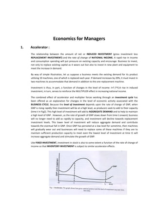
1.
Economics for Managers
1. Accelerator :
The relationship between the amount of net or INDUCED INVESTMENT (gross investment less
REPLACEMENT INVESTMENT) and the rate of change of NATIONAL INCOME. A rapid rise in income
and consumption spending will put pressure on existing capacity and encourage. Business to invest,
not only to replace existing capital as it wears out but also to invest in new plant and equipment to
meet the increase in demand.
By way of simple illustration, let us suppose a business meets the existing demand for its product
utilizing 10 machines, one of which is replaced each year. If demand increases by 20%, it must invest in
two machines to accommodate that demand in addition to the one replacement machine.
Investment is thus, in part, a function of changes in the level of income: I=f (^Y).A rise in induced
investment, in turn, serves to reinforce the MULTIPLIER effect in increasing national income.
The combined effect of accelerator and multiplier forces working through an investment cycle has
been offered as an explanation for changes in the level of economic activity associated with the
BUSINESS CYCLE. Because the level of investment depends upon the rate of change of GNP, when
GNP is rising rapidly then investment will be at a high level, as producers seek to add to their capacity
(time t in Fig2). This high level of investment will add to AGGREGATE DEMAND and to help to maintain
a high level of GNP . However, as the rate of growth of GNP slows down from time t onward, business
will no longer need to add as rapidly to capacity, and investment will decline towards replacement
investment levels. This lower level of investment will reduce aggregate demand and contribute
towards the eventual fall in GNP. Once GNP has persisted at a low level for sometime, then machines
will gradually wear out and businesses will need to replace some of these machines if they are to
maintain sufficient production capacity to meet even the lowest level of investment at time t1 will
increase aggregate demand and stimulate the growth of GNP.
Like FIXED INVESTMENT, investment in stock is also to some extent a function of the rate of change of
income so that INVENTORY INVESTMENT is subject to similar accelerator effects.

2.
2. Advertising:‐
A means of stimulating demand for a product and establishing strong BRAND LOYALTY .Advertising is
one of the main forms of PRODUCT DIFFERENCIATION competition and is used both to inform
perspective buyers of a brand’s particular attributes and to persuade them that the brand is superior
to competitor’s offerings.
There are to contrasting views of advertising’s effect on MARKET PERFORMANCE. Traditional ‘static’
market theory, on the one hand, emphasizes the misallocate effects of advertising. Here advertising is
depicted as being solely concerned with brand‐switching between competitors within a static overall
market demand and serves to increase total supply costs and the price paid by the consumer.
This is depicted in Fig.3 (a). (See PROFIT MAXIMIZATION).
The alternative view of advertising emphasizes its role as one of expanding market demand and
ensuring that firm’s demand is maintained at levels that enable them to achieve economics of large‐
scale production (SEE ECONOMICS OF SCALE).Thus ,advertising may be associated with a higher
market output and lower prices than allowed for in the static model. This is illustrated in Fig.3 (b).
3. Agency Cost
A form of failure in the contractual relationship between PRINCIPAL (the owner of a firm or other
assets) and an AGENT (the person contacted by the principal to manage the firm or other assets). This
failure arises because the principal cannot fully monitor the activities of the agent. Thus there is a

3.
possibility that an agent may not act in the interests of his principal, unless the principal can design an
appropriate reward structure for the agent that aligns that agent’s interests with those of the
principal.
Agency relations can exist between firms, for example, licensing and franchising arrangements
between the owner of a branded product (the principal) and licensees who wish to make and sell that
products. (Agents).However, agency relations can also exist within firms, particularly in the
relationship between the shareholders who own a public JOINT‐STOCK COMPANY (the principals) and
salaried professional managers who run the company (the agents.) Agency costs can arise from slack
effort by employees and the cost of monitoring and supervision designed to deter slack effort. See
PRINCIPAL‐AGENT THEORY, CONTRACT, TRANSACTION, DIVORCE OF OWNERSHIP FROM CONTROL,
MANAGERICAL THEORIES OF THE FIRM, TEAM PRODUCTION)
4. Aggregate Demand or Aggregate expenditure:‐
The total amount of expenditure (in nominal terms) on domestic goods and services. In the CIRCULAR
FLOW OF NATIONAL INCOME MODEL aggregate demand is made up of CONSUMPTION EXPENDITURE
(C), INVESTMENT EXPENDITURE(I), GOVERNMENT EXPENDITURE (G) and net EXPORTS (exports less
imports) (E):
Aggregate demand = C + I + G + E
Some of the components of aggregate demand are relatively stable and change only slowly over time.
(eg: consumption expenditure); others are much more volatile and change rapidly, causing fluctuations
in the level of economic activity(eg: investment expenditure).
In 2003, consumption expenditure accounted for 52%, investment expenditure accounted for 13%,
government expenditure accounted for 15% and exports accounted for 20% of gross final
expenditure(GFE) on domestically produced output. (GFE minus imports=GROSS DOMESTIC
PRODUCT) See Fig.133(a) NATIONAL INCOME ACCOUNTS.
Aggregate demand interacts with AGGREGATE SUPPLY to determine the EQUILIBRIUM LEVEL OF
NATIONAL INCOME. Government seeks to regulate the level of aggregate demand in order to
maintain FULL EMPLOYMENT, avoid INFLATION, promote ECONOMIC GROWTH and secure BALANCE‐
OF‐PAYMENTS EQULIBRIUM through the use of FISCAL POLICY AND MONETARY POLICY. See
AGGREGATE DEMAND SCHEDULE, ACTUAL GROSS NATIONAL PRODUCTS DEFLATIONARY GAP,
INFLATIONARY GAP, BUSINESS CYCLE, STABILIZATION POLICY, POTENTIAL GROSS NATIONAL
PRODUCT.
5. Aggregate Demand Schedule:‐
A Schedule depicting the total amount of spending on domestic goods and services of various levels of
NATIONAL INCOME. It is constructed by adding together THE CONSUMPTION, INVESTMENT, &

4.
GOVERNMENT EXPEENDITURE and exports schedules, as indicated in fig 4(a).
A given aggregate demand schedule is drawn up on the usual CETERIS PARIBUS conditions. IT WILL
SHIFT UPWARDS OR DOWNWARDS IF SOME DETERMINING FACTOR CHANGES. See Fig 4(b).
Alternatively ,the aggregate demand schedule can be expressed in terms of various levels of national
income demanded at each PRICE LEVEL as shown in Fig 4( C ).This alternate schedule is also drawn on
the assumption that influences on spending plans are constant. It will shift rightwards or leftwards if
some determining factors change. See Fig 4(d)..This version of the aggregate demand schedule and
DEMAND CURVE for an individual product, although in this case the schedule represents demand for
all goods and services and deals with the general price level rather than with a particular price.
National Income

6.
6. Aggregate Supply:
The total amount of domestic goods and services supplied by businesses and government, including
both consumer products and capital goods. Aggregate supply interacts with AGGREGATE DEMAND to
determine the EQUILIBRIUM LEVEL OF NATIONAL INCOME. (see AGGREGATE SUPPLY SCHEDULE).
In the short term, aggregate supply will tend to vary with the level of demand for goods and services,
although the two need not correspond exactly. For example, businesses could supply more products
than are demanded in the short term, the difference showing up a build‐up of unsold stocks.
(unintended INVENTORY INVESTMENT).On the other hand, businesses could supply fewer products
than are demanded in the short term, the difference being met by running down stocks. However
discrepancies between aggregate supply and aggregate demand cannot be very large or persist for
long, and generally businesses will offer to supply output only if they expect spending to be sufficient
to sell all that output.
Over the long term, aggregate supply can increase as a result of increases in the LABOUR FORCE,
increases in CAPITAL STOCK and improvements in labour PRODUCTIVITY. See ACTUAL GROSS
NATIONAL PRODUCT, POTENTIAL GROSS NATIONAL PRODUCT, and ECONOMIC GROWTH.
7. Aggregate Supply Schedule
A schedule depicting the total amount of domestic goods and services, supplied by businesses and
government at various levels of total expenditure. The AGGREGATE SUPPLY schedule is generally
drawn as a 45⁰ line because business will offer any particular level of national output only if they
expect total spending (AGGREGATE DEMAND) to be just sufficient to sell all of that output. Thus, in
Fig 5(a), £100 million of expenditure calls forth £100 million of aggregate supply, £200 million of
expenditure calls forth £200 million of aggregate supply, and so on. This process cannot continue
indefinitely.
However, for once an economy’s resources are fully employed in supplying products then additional
expenditure cannot be met from additional domestic resources because the potential output ceiling
of the economy has been reached . Consequently, beyond the full‐employment level of national
product (f), the aggregate supply schedule becomes vertical. See POTENTIAL GROSS NATIONAL
PRODUCT, ACTUAL GROSS NATIONAL PRODUCT.
Alternatively, the aggregate supply schedule can be expressed in terms of various levels of real
national income supplied at each PRICE LEVEL as shown in Fig 5(b).This version of the aggregate
supply schedule parallels at the macro level the supply schedule and SUPPLY CURVE for an individual
product, though in this case the schedule represents the supply of all goods and services and deals
with the general price level rather than a particular product price. Fig 5(c) shows a shift of the
aggregate supply curve to the right as a result of, for example, increases in the labour force or capital
stock and technological advances. Aggregate supply interacts with aggregate demand to determine
the EQUILIBRIUM LEVEL OF NATIONAL INCOME.

7.
8. Allocative Efficiency:‐
An aspect of MARKET PERFORMANCE that denotes the optimum allocation of scarce resources
between end users in order to produce that combination of goods and services that best accords with
the pattern of consumer demand. This is achieved when all market prices and profit levels are
consistent with the real resource costs of supplying products. Specifically, consumer welfare is
optimized when for each product the price is equal to the lowest real resource cost of supplying that
product, including a NORMAL PROFIT reward to suppliers. Fig.7 (a) depicts a normal profit equilibrium
under conditions of PERFECT COMPETITION with price being determined by the intersection of the
market supply and demand curves and with MARKET ENTRY/MARKET EXIT serving to ensure that
price (P) is equal to minimum supply cost in the long run (AC).

8. By contrast, where some markets are characterized by monopoly elements, then in these markets
output will tend to be restricted so that fewer resources are devoted to producing these products than
the pattern of consumer demand warrants. In these markets, prices and profit levels are not
consistent with the real resource costs of supplying the products. Specifically, in MONOPOLY markets
the consumer is exploited by having to pay a price for a product that exceeds the real resource cost of
supplying it, this excess showing up as an ABOVE‐NORMAL PROFIT for the monopolist. Fig.7(b) depicts
the profit maximizing price‐output combination for a monopolist, determined by equating marginal
cost and marginal revenue. This involves a smaller output and a higher price than would be the case
under perfect competition, with BARRIERS TO ENTRY serving to ensure that the output restriction and
excess prices persist over the long run. See PARETO OPTIMALITY, MARKET FAILURE.
9. Arc Elasticity:‐
A rough measure of the responsiveness of DEMAND OF SUPPLY to changes in PRICE, INCOME, etc. In
the case of PRICE ELASTICITY OF DEMAND, it is the ratio of the percentage change in quantity
demanded (Q) to the percentage change in price (P) over a price range such as P0 to P1 in Fig. 8. Arc
elasticity of demand is expressed notationally as:
e=(Q1‐Q2)*(P1+P0)/(P1‐P0)(Q1+Q0)

9. where P0 = original price, Q0 = original quantity, P1 = new price Q1 = new quantity. Because are elasticity
measures the elasticity of demand (e) over a price range or arc of the demand curve, it is only an
approximation of demand elasticity at a particular price (POINT ELASTICITY). However, the arc elasticity
formula gives a reasonable degree of accuracy in approximating point elasticity when price and/or
quantity changes are small. See also ELASTICITY OF DEMAND.
10. Asset Value Theory of exchange rate determination
an explanation of the volatility of EXCHANGE‐RATE movements under a FLOATING EXCHANGE‐RATE
SYSTEM. Whereas the PURCHASING‐POWER PARITY THEORY suggests that SPECULATION is
consistent with the achievement of BALANCE‐OF‐PAYMENTS EQUILIBRIUM, the asset‐value theory
emphasizes that, in all probability, it will not be. In this theory, the exchange rate is an asset price, the
relative price at which the stock of money, bills and bonds, and other financial assets of a country will
be willingly held by foreign and domestic asset holders. An actual alteration in the exchange rate or a
change in expectations about future rates can cause asset holders to alter their portfolios. The
resultant change in demand for holdings of foreign currency relative to domestic currency assets can
at times produce sharp fluctuations in exchange rates. In particular, uncertainty about future market
rates and the unwillingness of banks and other large financial participants in the foreign‐exchange
markets to take substantial positions in certain currencies, especially SOFT CURRENCIES, may diminish
funds for stabilizing speculation that would in turn diminish or avoid erratic exchange‐rate
movements.
If this should prove the case, then financial asset‐switching is likely to reinforce and magnify
exchange‐rate movements initiated by current account transactions (i.e. changes in imports and
exports), and in consequence may produce exchange rates that are inconsistent with effective overall
balance‐of‐payments equilibrium in the longer run.
11. Autonomous Consumption
That part of total CONSUMPTION expenditure that does not vary with changes in NATIONAL INCOME
or DISPOSABLE INCOME. In the short term, consumption expenditure consists of INDUCED

10. CONSUMPTION (consumption expenditure that varies directly with income) and autonomous
consumption. Autonomous consumption represents some minimum level of consumption
expenditure that is necessary to sustain a basic standard of living and which consumers would
therefore need to undertake even at zero income. See CONSUMPTION SCHEDULE.
12. Autonomous Investment
That part of real INVESTMENT that is independent of the level of, and changes in, NATIONAL
INCOME. Autonomous investment is mainly dependent on competitive factors such as plant
modernization by businesses in order to cut costs or to take advantages of a new invention. See
INDUCED INVESTMENT, INVESTMENT SCHEDULE.
13. Average cost (long run) & (Short run)
The unit cost (TOTAL COST divided by number of units produced) of producing outputs for plants of
different sizes. The position of the SHORT‐RUN average total cost (ATC) curve depends on its existing
size of plant. In the long run, a firm can alter the size of its plant. Each plant size corresponds to a
different U‐shaped short‐run ATC curve. As the firm from one curve to another. The path along with
the firm expands – the LONG‐RUN ATC curve – is thus the envelope curve of all the possible short‐run
ATC curves. See Fig. 10(a).
It will be noted that the long‐run ATC curve is typically assumed to be a shallow U‐shape, with a least‐
cost point indicated by output level OX. To begin with the, average cost falls (reflection ECONOMIES
OF SCALE); eventually, however, the firm may experience DIS ECONOMIES OF SCALE and average cost
begins to rise.
Empirical studies of companies’ long‐run average‐cost curves, however, suggest that diseconomies of
scale are rarely encountered within the typical output ranges over which companies operate, so that
most companies’ average cost curves are L‐shaped, as in Fig.10(b). In cases where diseconomies of
scale are encountered, the MINIMUM EFFICIENT SCALE at which a company will operate corresponds
to the minimum point of the long‐run average cost curve (Fig.10(a)). Where diseconomies of scale are
not encountered within the typical output range, minimum efficient scale corresponds with the
output at which economies of scale are exhausted and constant returns of scale begin (Fig.10(b)).
Compare AVERAGE COST (SHORT‐RUN).

11. The average cost (short run) is the unit cost (TOTAL COST divided by the number of units produced ) of
producing particular volumes of output in a plant of a given fixed size.
Average total cost (ATC) can be split up into average FIXED COST (AFC) and average VARIABLE COST.
AFC declines continuously as output rises as a given amount of fixed cost is ‘spread’ over a greater
number of units. For example with fixed costs of £1,000 per year and annual output of 1000 units, fixed
costs per unit would be £1, but if annual output rose to 2000 units, the fixed cost per unit would fall to
50 pence – see AFC curve in Fig 11 (a).
Overt he whole potential range within which a firm can produce, AVC falls at first, (reflecting increasing
RETURNS TO THE VARIABLE FACTOR INPUT output increases faster than costs) but then rises (reflecting
DIMINISHING RETURNS to the variable returns – costs increase faster than output) as shown by the
AVC curve. Thus the conventional short‐run ATC curve is U‐shaped
Over the more restricted output range in which firms typically operate, however, constant returns to
the variable input are more likely to be experienced, where, as more variable inputs are added to the
fixed inputs employed in production, equal increments in output result. In such circumstances AVC will
remain constant over the whole output range and as a consequence ATC will decline in parallel with
AFC. .
14. Average prosperity to consume , import , save ,tax(APC)
The fraction of a given level of NATIONAL INCOME that is spent on consumption:

12. Alternatively, consumption can be expressed as a proportion of DISPOSABLE INCOME. See
CONSUMPTION EXPENDITURE, PROPENSITY TO CONSUME, MARGINAL PROPENSITY TO CONSUME.
Average propensity to import (APM) the fraction of a given level of NATIONAL INCOME that is spent
on IMPORTS:
Alternatively, imports can be expressed as a proportion of DISPOSABLE INCOME. See also
PROPENSITY TO IMPORT, MARGINAL PROPENSITY TO IMPORT.
average propensity to save (APS) the fraction of a given level of NATIONAL INCOME that is saved (see
SAVING):
Alternatively, saving can be expressed as a proportion of DISPOSABLE INCOME. See also PROPENSITY
TO SAVE, MARGINAL PROPENSITY TO SAVE.
average propensity to tax (APT) the fraction of a given level of NATIONAL INCOME that is
appropriated by the government in TAXATION:
See also PROPENSITY TO TAX, MARGINAL PROPENSITY TO TAX, AVERAGE RATE OF TAXATION.
15. Balance of payments equilibrium:‐
A situation where, over a run of years, a country spends, and invests abroad no more than other
countries spend and invest in it. Thus, the country neither adds to its stock of INTERNATIONAL
RESERVES, nor sees them reduced.
In an unregulated world it is highly unlikely that external balance will always prevail, Balance of
payments deficits and surpluses will occur, but provided they are small, balance‐of‐payments
disequilibrium can be readily accommodated. The main thing to avoid is a FUNDAMENTAL
DISEQUILIBRIUM – a situation of chronic imbalance.
There are three main ways of restoring balance‐of‐payments equilibrium should an imbalance occur:
(a) external price adjustments. Alterations in the EXCHANGE RATE between currencies involving
(depending upon the particular exchange‐rate system in operation) the DEVALUATION/DEPRECIATION
and REVALUATION/APPRECIATION of the currencies concerned to make exports cheaper/more
expensive and imports dearer/less expensive in foreign currency terms. For example, with regard to

13. exports, in Fig.14(a), if the pound‐dollar exchange rate is devalued from $1.60 to $1.40 then this would
allow British exporters to reduce their prices by a similar amount, thus increasing their price
competitiveness in the American market.
(b) internal price and income adjustments. The use of deflationary and reflationary (see DEFLATION,
REFLATION) monetary and fiscal policies to alter the prices of domestically produced goods and services
vis‐à‐vis products supplied by other countries so as o make exports relatively cheaper/dearer and
imports more expensive/cheaper in foreign currency terms. For example, again with regard to exports,
if it were possible to reduce the domestic price of a British product, as shown in Fig.14(b), given an
unchanged exchange rate, this would allow the dollar price of the product in the American market to be
reduced, thereby improving its price competitiveness vis‐à‐vis similar American products. The same
policies are used to alter the level of domestic income and spending, including expenditure on imports.
(c) Trade and foreign exchange restrictions. The use of TARIFFS, QUOTAS, FOREIGN‐EXCHANGE
CONTROLS, etc., to affect the price and availability of goods and services, and of the currencies with
which to purchase these products.
Under a FIXED EXCHANGE‐RATE SYSTEM, minor payments imbalances are corrected by appropriate
domestic adjustments (b), but fundamental disequilibriums require, in addition, a devaluation or
revaluation of the currency (a). It must be emphasized, however, that a number of favorable conditions
must be present to ensure that success of devaluations and revaluations (see DEPRECIATION 1 for
details).
In theory, a FLOATING EXCHANGE‐RATE SYSTEM provides an ‘automatic’ mechanism for removing
payments imbalances in their incipiency (that is, before they reach ‘fundamental’ proportions): a deficit
results in an immediate exchange‐rate depreciation, and a surplus results in an immediate appreciation
of the exchange rate (see PURCHASING‐POWER PARITY THEORY). Again, however, a number of
favourable conditions must be present to ensure the success of depreciations and appreciations. See
also ADJUSTMENT MECHANISM, J‐CURVE, INTERNAL‐EXTERNAL BALANCE MODEL, MARSHALL‐
LERNER CONDITION, TERMS OF TRADE.
16. Bank deposit creation or…or money multiplier
The ability of the COMMERCIAL BANK SYSTEM TO create new bank deposits and hence the MONEY
SUPPLY. Commercial banks accept deposits of CURRENCY from the general public. Some of this money
is retained by the banks to meet day‐to‐day withdrawals (see RESERVE ASSET RATIO).The remai9nder
of the money is used to make loans or is invested. When a bank on‐lends, it creates additional deposits
in favour of borrowers. The amount of new deposits the banking system as a whole can create depends
on the magnitude of the reserve‐asset ratio. In the example set out in Fig.15, the banks are assumed to
operate with a 50% reserve‐asset ratio.Bank1 receives initial deposits of £100m million from the general
public. It keeps £50 million for liquidity purposes and on‐lends £50 million. This £50 million, when spent,
is redeposited with Bank2; Bank2 keeps £25 million as part of its reserve assets and on‐lends £25
million; and so on. Thus, as a result of an initial deposit of £100 million, the banking system has been
able to ‘create’ credit makes it a prime target for the application of MONETARY POLICY as a means of
regulating the level of spending in the economy.

14.
17. Bilateral monopoly :‐
A market situation comprising one seller(like MONOPOLY) and one buyer (like MONOPSONY).
18. Bilateral oligopoly:‐
A market situation with a significant degree of seller concentration (like OLIGOPOLY) and a significant
degree of buyer concentration (like OLIGOPSONY).see COUNTERVAILING POWER.
19. Bounded Rationality:‐
Limits on the capabilities of people to deal with complexity, process information and pursue rational
aims, Bounded rationality prevents parties to a CONTRACT from contingency that might arise during a
TRANSACTION, so preventing them from writing complete contracts.
20. Budget Line or consumption possibility line:‐
A line showing the alternative combinations of goods that can be purchased by a consumer with a given
income facing given prices. See Fig 19.See also CONSUMER EQUILIBRIUM, REVEALED PREFERENCE
THEORY, PRICE PERFECT.

15.
21. Business Cycle or Trade Cycle:‐
FLUCTUATIONS IN THE LEVEL OF ECONOMIC ACTIVITY (actual gross NATIONAL PRODUCT), alternating
between periods of depression and boom conditions.
The business cycle is characterized by four phases (see Fig.20):
a) DEPRESSION, a period of rapidly falling AGGREGATE DEMAND accompanied by very low levels of
output and heavy UNEMPLOYMENT, which eventually reaches the bottom of the trough)
b) RECOVERY, an upturn in aggregate demand accompanied by rising output and a reduction in
unemployment;
c) BOOM, aggregate demand reaches and then exceeds sustainable output levels (POTENTIAL GROSS
NATIONAL PRODUCT)s the peak of the cycle is reached. Full employment is reached and the emergence
of excess demand causes the general price level to increase(see INFLATION);
d) RECESSION, the boom comes to an end and is followed by recession Aggregate demand falls,
bringing with it, initially modest falls in output and employment but then, as demand continues to
contract, the onset of depression.
What causes the economy to fluctuate in this way? One prominent factor is the volatility of FIXED
INVESTMENT expenditures (the investment cycle), which are themselves a function of businesses
‘EXPECTATIONS about future demand. At the top of the cycle. Income begins to level off and
investment n new supply capacity finally ‘catches up’ with demand (see ACCELERATOR).This causes a
reduction in INDUCED INVESTMENT and, via contracting MULTIPLIER effects. Leads to a fall in national

16. income, which reduces investment even further. At the bottom of the depression, investment may rise
exogenously(because ,for example, of the introduction of new technologies) or through the revival of
REPLACEMENT INVESTMENT, in this case, the increase in investment spending will, via expansionary
multiplier effects, leads to an increase in national income and a greater volume of induced investment.
SEE ALSO DEMAND MANAGEMENT, KONDRATIEFF CYCLE, AND SECULAR STAGNATION.
22. Capital‐Output Ratio:‐
The measure of how much additional CAPITAL is required to produce each extra unit of OUTPUT, or,
put the other way round, the amount of extra output produced by each unit of added capital. The
capital‐output ratio indicates how ‘efficient new INVESTMENT is in contributing to ECONOMIC
GROWTH. Assuming, for example, a 4:1 capital‐output ratio, each four units of extra investment
enables national output to grow by one unit. If the capital‐output ratio is 2:1, however, then each two
units of extra investment expands national income by one unit. See CAPITAL ACCUMULATION,
PRODUCTIVITY .See also SOLLOW ECONOMIC‐GROWTH MODEL.
23. Cartel: ‐
A form of collusion between a group of suppliers| aimed at suppressing competition between
themselves, wholly or in part .Cartels can take a number of forms. For example, suppliers may set up a
sole Selling agency that buys up their individual output at an agreed price and arranges for the
marketing of these products on a coordinated basis. Another variant is when Suppliers operate an
agreement (see RESTRICTIVE TRADE AGREEMENT) that sets uniform selling price for their products,
thereby suppressing price competition but with suppliers then competing for market share through
PRODUCT DIFFERENCIATION strategies. A more comprehensive version of a cartel is application not
only of common selling prices and joint marketing but also restrictions on production, involving the
assignment of specific output quotas to individual suppliers, and coordinated over‐capacity or
extending capacity on a coordinated basis. cartels are usually established with the purpose of either
exploiting the joint market powers of suppliers to extract MONOPOLY profits or as a means of
preventing cut‐throat competition from forcing firms to operate at a loss, often resorted to in times of
depressed demand(also called 'crisis cartel').In the former case, central administration agency could
determine the price and output of the industry, and the output quotas of each of the separate
member firms, in such a way as to restrict total industry output and maximize the joint profits of the
group. Price and output will thus tend to approximate those of profit‐maximizing monopolist. See Fig.2a
A number of factors are crucial to the successful operation of a cartel in particular the participation
of all significant suppliers of the product and their full compliance with the policies of the cartel. Over‐
participation of some key suppliers and 'cheating' by cartel members, together with the ability of buyers
to switch to substitute products, may well serve to undermine a cartel's ability to control prices. In
many countries, including the UK, the USA and the European Union, cartels concerned with price
fixing, market sharing and restrictions on production and capacity are prohibited by law. See capacity
is prohibited by law. See COMPETITION POLICY (UK), COMPETITION POLICY (EU), ORGANIZATION OF
PETROLEUM‐EXPORTING COUNTRIES (OPEC).

17.
24. Circular flow of National Income Model:‐
A simplified exposition of money and physical or real flows through the economy that serves
as the basis for macroeconomic analysis. In Fig 22(a) the solid lines show how, in monetary
terms HOUSEHOLDS purchase goods and services from BUSINESSES using income received
from supplying factor inputs to businesses (CONSUMPTION EXPENDITURE) .In physical
terms(shown by the broken lines),businesses produce goods and services using factor inputs
supplied to them by households.
The basic model can be developed to incorporate a number of “INJECTIONS’ to, and
‘WITHDRAWALS’ from, the income flow. In Fig 22(b) not all the income received by
households is spent‐some is saved. SAVINGS is a ‘withdrawal’ from the income flow.
INVESTMENT expenditure ‘injects’ funds into the income flow. Part of the income accruing to
households is taxed by the government and serves to reduce disposable income available for
consumption expenditure. TAXATION is a ‘withdrawal’ from the income flow. GOVERNMENT
EXPENDITURE on products and factor inputs ‘injects’ funds into the income flow. Households
spend some of their income on imported goods and services. On the other hand, some output
is sold to overseas customers. EXPORTS represent a demand domestically produced goods and
services and hence constitute an ‘injection’ into the income flow. See also AGGREGATE
DEMAND, EQUILIBRIUM LEVEL OF NATIONAL INCOME MODEL.

18. 25. Closed Economy:‐
An economy that is not influenced by any form of INTERNATIONAL TRADE, that is, there are no
EXPORTS or IMPORTS of any kind. By concentrating on a closed economy, it is possible to simplify the
CIRCULAR FLOW OF NATIONAL INCOME MODEL and focus upon income and expenditure within an
economy.
In terms of the circular flow, AGGREGATE DEMAND in a closed economy is represented by
Y=C+I+G
Where Y=national Income
C=consumption Expenditure
I=investment expenditure
G=government expenditure.
By contrast, the OPEN ECONOMY allows for the influence of imports and exports and here aggregate
demand is represented in the circular flow as:‐
Y=C+I+G+(X‐M)
Where X=exports
M=imports
26. Cobb‐Douglas production function:‐
A particular physical relationship between OUTPUT of products and FACTOR INPUTS (LABOUR AND
CAPITAL) used to produce these outputs. This particular form of the PRODUCTION FUNCTION suggests

19. that where there is effective competition in factor markets the ELASTICITY OF TECHNICAL
SUBSTITUTION between labour and capital will be equal to one ; that is labour can be substituted for
capital in any given proportions, and vice versa, without affecting output.
The Cobb‐Douglas production function suggests that the share of labour input and the share of capital
input are relative constants in an economy, so that although labour and capital inputs may change in
absolute terms, the relative share between the two inputs remains constant. See PRODUCTION
POSSIBILITY BOUNDARY, CAPITAL‐LABOUR RATIO, PODUCTION FUNCTION, CAPITAL‐INTENSIVE
FIRM/INDUSTRY, ISOQUANT CURVE, ISOQUANT MAP.
27. Cobweb Theorem:‐
A Theory designed to explain the path followed in moving toward an equilibrium situation when there
are lags in the adjustments of either SUPPLY or DEMAND to changes in prices, COMPARATIVE STATIC
EQUILIBRIUM ANALYSIS predicts the effect of demand or supply changes by comparing the original
equilibrium price and quantity with the new equilibrium that results. The cobweb theorem focuses
upon the dynamic process of adjustment in markets by tracing the path of adjustment of prices and
output in moving from one equilibrium situation toward another (see DYNAMIC ANALYSIS).
The cobweb theorem is generally used to describe oscillations in prices in agricultural markets where
the delay between, for example, planting and harvesting means that supply reacts to prices with time
lag. The simplest case where current quantity demanded responds to current price while current
quantity supplied depends upon price in the previous period is depicted in Fig 23.In the figure D(t)
denotes quantity demanded in the current period, S(t),denotes quantity supplied ,while price is
denoted by P(t),and price in the previous period is denoted by P(t‐1).If demand were to fall rapidly, such
that the demand curve shifted left from D(t) to D1(t),then comparative static analysis suggests that the
market will eventually move from `equilibrium point E (with price OP1 and quantity OQ1)to equilibrium
point E1(with price OP4 and quantity 0Q4).Dynamic analysis suggest that the path followed will be less
direct than this.
Starting from the original equilibrium price OP1,which has prevailed in years t‐1 and t, farmers will have
planned to produce quantity OQ1.However ,after the contraction in demand in year t, supply will
exceed demand by QQ1,and in order to sell all the quantity OQ1 coming onto the market, price has fall
to OP2.The lower price OP2,which prevails in year t, will discourage farmers from producing and they
will reduce acreage devoted to this crop so that in the next year t+1 a much smaller quantity OQ2 is
supplied.
In year t+1, and at price OP2, demand now exceeds supply by the amount Q1Q2, and in order to ration
the limited supply OQ2 that is available, price will rise to OP3.This higher price in year t+1 will
encourage farmers to increase their acreage planted so that in the following year t+2,a large quantity
OQ3 will be supplied, which means that in year t+2 supply exceeds demand and price will fall below
OP3,which will discourage planting for the following year, and so on. The eventual result of this process
of adjustment is that a new equilibrium is achieved at E1 but only after a series of fluctuating prices in
intermediate periods are experienced. See AGRICULTURAL POLICY.

20.
28. Concentration Measures:‐
The measures of the size distribution of firms engaged in economic activities.
The broadest concentration measure is the aggregate concentration measure, which looks at the share
of total activity in the economy accounted for by the large firms, for example, the proportion of total
industrial output accounted for by the largest 200 firms; or the share of total manufacturing output
produced by the 100 largest companies. Various size criteria may be used for this measure, in particular
, sales , output ,numbers employed and capital employed, each of which can give slightly different
results because of differences in capital intensity. Such measures serve to give an overall national view
of concentration and how it is changing over time.
Although aggregate concentration measures are useful, they are generally too broad for purposes of
economic analysis where interest focuses upon markets and performance in these markets
.Consequently, economists have developed several measures of MARKET concentration and that seek
to measure SELLER OR BUYER CONCENTRATION. The most common of these measures is the
CONCENTRATION RATIO, which records the percentage of a market’s sales accounted for by a given
number of the largest firms in that market. In the UK it has been usual to estimate the concentration
ratio for the three or (most recently) five largest firms, whereas in the USA the four‐firm concentration
ratio tends to be employed.
The concentration ratio, however, records only seller concentration at one point along the cumulative
at one point concentration curve, as Fig.28 (a) indicates. This makes it difficult to compare
concentration curve for two different markets, like A and B in the figure, where their concentration
curves intersect. For example, using a three firm concentration ration, market A is more concentrated
while using a five‐firm concentration ratio shows market B to be concentrated. An alternative
concentration index, called the HERFINDAHL INDEX, gets around this problem by taking into account
the number and market shares of all firms in the market. The Herfindahl index is calculated by summing

21.
the squared market shares of all firms. The index can vary between a value of zero (where there are
large number of equally sized firms)and one(where there is just one firm).
Concentration measures, like the concentration ratio and the Herfindahl index, are known as absolute
concentration measures since they are concerned with market rates of a given (absolute) number of
firms. By contrast, relative concentration measures are concerned with inequalities in the share of total
firms producing for the market. Such irregularities can be recorded in the form of a Lorenz curve as in
Fig.28(b).The diagonal straight line shows what a distribution of complete quality in firm shares would
look like, so the extent to which the Lorenz CURVE DEVIATES FROM THIS LINE GIVES AN INDICATION
OF RELATIVE SELLER CONCENTRATION. For example, the diagonal line shows how we might expect 50%
of market sales to be accounted for by 50% of the total firms, whilst in fact 50‐% of the market sales are
accounted for by the largest 25% of total firms, as the Lorenz curve indicates. The Gini coefficient
provides a summary measure of the extent to which the Lorenz curvefor a particular market deviates
from the linear diagonal. It indicates the extent of the bow‐shaped area in the figure by dividing the
shaded area below the Lorenz curve by the area above the line of equality. The value of the Gini
coefficient ranges from zero (complete equality)to one (complete inequality).
In practice, most market concentration studies use concentration ratios calculated from data derived
from the census of production.
Concentration measures are widely used in economic analysis and for purposes of applying
COMPETITION POLICY to indicate the degree of competition or monopolization present in a market.
They need to be treated with caution, however. On the one hand, they may overstate the extent of
monopolization.First,the boundaries of the market may be defined too narrowly(for example, the ‘beer
market’)when it might be more appropriate to adopt a wider interpretation of what constitutes the
relevant market by including actual and potential substitutes (for example, the ‘alcoholic drink market’,
which includes also spirits and wines).Thus ,calculating a firm’s market share in terms of the beer
market alone may make it seem more powerful than it actually is . Secondly, concentration ratios are
usually compiled by reference to the output of domestic suppliers, thus ignoring the competition
afforded by imports. Thirdly, market concentration is only one element of market structure. If
BARRIERS TO ENTRY to the market are relatively low, or suppliers are confronted by powerful buyers,
again the market may well be much more competitive than shown by the concentration ratio. On the
other hand, concentration ratios may understate the degree of monopolization. First, the market may
be defined too broadly when a narrower specification of the market’s boundaries may be more
appropriate. This can be important in the context of suppliers who deliberately choose to ‘focus’ on a
narrow segment of the market(See COMPETITIVE STRATEGY).Secondly, conduct elements as well as
structure variables need to be considered. For example, while superficially a market with a low or
moderate degree of seller concentration may appear to be competitive, in practice it may be highly
monopolistic because the suppliers have set up a price‐fixing CARTEL.
Thus, looked at ‘in the round’, concentration ratios are but one aspect in examining the dynamics of a
market and whether or not it exhibits competitive or monopolistic tendencies.

22.
29. Concentration Ratio:‐
A measure of the degree of SELLER CONCENTRATION in a MARKET. The concentration ratio shows the
percentage of market sales accounted for by, for example, the largest four firms or largest eight firms.
The concentration ratio is derived from the market concentration curve, which can be plotted on a
graph, with the horizontal scale showing the number of firms cumulated from the largest size and
vertical scale showing the cumulative percentage of market sales accounted for by particular number of
firms. See Fig 29.See CONCENTRATION MEASURES, MARKET STRUCTURE.

23.
30. Consumer’s Surplus:‐
The extra satisfaction or UTILITY gained by consumers from paying an actual price for a good that is
lower than that which they would have been prepared to pay. See Fig.32(a).The consumer’s surplus is
maximized only in PERFECT COMPETITION, where price is determined by the free play of market
demand and supply forces and all consumers pay the same price. Where market price is not determined
by demand and supply forces in competitive market conditions but is instead determined
administratively by a profit‐maximizing MONOPOLIST, then the resulting restriction in market output
and the increase in market price cause a loss of consumer surplus, indicated by the shaded area
PP(m)XE in Fig.32(b).If DISCRIMINATING MONOPOLIES were able to charge a separate price to each
consumer that reflected the maximum amount that the consumer was prepared to pay, then the
monopolist would be able to appropriate all the consumer surplus in the form of sales revenue.
Business strategists can use the concept of the consumer’s surplus to increase the firm’s profit (See
VALUE‐CREATED MODEL).To illustrate: you are a Manchester United Football fan; tickets for a home
game are currently priced at £50 but you would be willing to pay £75.Hence you have ‘received’ as a
consumer ‘perceived benefit’ or ‘surplus’ of £25 over and above the price actually charged. Manchester
United, however ,instead of charging a single price of £50 could segment its market by charging
different prices for admission to different parts of the ground(see PRICE DISCRIMINATION, MARKET
SEGMENTATION) in order to ‘capture most of the consumers’ surplus for itself . Thus, it could continue
to charge the ‘basic’ price of £50 for admission to certain parts of the ground. £75 for seating in the
main stand and £120 for an ‘executive box’ seat. Compare PRODUCER’S SURPLUS. See DIMINISHING
MARGINAL UTILITY,DEAD WEIGHT LOSS.

24. 31. Consumption Schedule
A schedule depicting the relationship between CONSUMPTION EXPENDITURE and the level of
NATIONAL INCOME OR DISPOSAL INCOME, also called consumption function. At low levels of
disposable income, households consume more than their current income (see DISSAVING), drawing on
past savings, and borrowing or selling assets in order to maintain consumption at some desired
minimum level (AUTONOMOUS CONSUMPTION).At higher levels of disposable income, they consume a
part of their current income and save the rest. See fig 33.See INDUCED CONSUMPTION).

25. 32. Cost Push Inflation:‐
A GENERAL INCREASE in prices caused by increases IN FACTOR INPUT costs. Factor input costs may rise
because raw materials and energy costs increase as a result of world‐wide shortages or the operation of
CARTELS(oil, for example) and where a country’s EXCHANGE RATE falls(see DEPRECIATION 1),or
because WAGE RATES in the economy increase at a faster rate than output per man
(PRODUCTIVITY).In the latter case, institutional factors, such as the use of COMPARABILITY and WAGE
DIFFERENTIAL arguments in COLLECTIVE BARGAINING and persistence of RESTRICTIVE LABOUR
PRACTICES, can serve to push up wages and limit the scope for productivity improvements. Faced with
increased input costs, producers try to ‘pass on’ increased costs by charging higher prices. In order to
maintain profit margins, producers would need to pass on the full increased costs in the form of higher
prices, but whether they are able to depend upon PRICE ELASTIITY OFDEMAND for their products.
Important elements in cost –push inflation in the UK and elsewhere have been periodic ‘explosions’ in
commodity prices(the increases in the price of oil in 1973,1979 and 1989 being cases in point),but more
particularly ‘excessive’ increases in wages/earnings. Wages/earnings account for around 77% of total
factor incomes (see FUNCTIONAL DISTRIBUTION OF INCOME.) and are a critical ingredient of
AGGREGATE DEMAND in the economy. Any tendency for money wages/earnings to outstrip underlying
PRODUCTIVITY growth (i.e. the ability of the economy to ‘pay for/absorb’ higher wages &
corresponding increases in the output) is potentially inflationary.
In the past PRICES AND INCOME POLICES have been used to limit pay awards. At the present time,
policy is mainly directed towards creating a low inflation economy (see MONTETARY POLICY,
MONETARY POLICY COMMITTEE), thereby reducing the imperative for the workers, rough their trade

26. unions, to demand excessive wage/earnings increases to compensate themselves for fall in their real
living standards.
The Monetary Policy Committee, in monitoring inflation, currently operates a ‘tolerance threshold’ for
wage/earnings growth of no more than 4 1/2 % as being compactible with low inflation(this figure
assumes productivity growth of around 2 ¾‐3 %).See INFLATION,INFLATIONARY SPIRAL,COLLECTIVE
BARGAINING.
32. Cross Elasticity of Demand:‐
A measure of the degree of responsiveness of the DEMAND for one good to a given change in the PRICE
of some other good.
(i) cross‐elasticity of demand = % change in quantity demanded of good A
% change in quantity demanded of good B
Products may be regarded by consumers as substitutes for one another, in which case a rise in the price
of good B (tea, for example) will tend to increase the quantity demanded of good A.(coffee, for
example). Here the cross‐elasticity of demand will be positive ' since as the price of B goes up the
quality demanded of A rises as consumers now buy more A in preference to the more expensive B, (ii)
cross‐elasticity of demand= % change in quantity demanded of good C / %change in price of good B .
Alternatively, products may be regarded by consumers as complements that are jointly
demanded, in which case a rice in the price of good B (tea ,for example)will tend to decrease not only
the quantity demanded of good B but also another good C (sugar, for example). Here the cross‐elasticity
of demand will be negative
Since a rise in the price of B serves to reduce the quantity demanded of C.
33. Deflation:‐
A reduction in the level of NATIONAL INCOME and output usually accompanied by a fall in the general
price level. (DISINFLATION).
A deflation is often deliberately brought about by the authorities in order to reduce INFLATION and to
improve the BALANCE OF PAYMENTS by reducing import demand. Instruments of deflationary policy
include fiscal measures (e.g.:‐tax increases) and monetary measures (e.g.:‐high interest rates).See
MONETARY POLICY, FISCAL POLICY.
34. Deflationary Gap:‐
The shortfall in total spending (AGGREGATE DEMAND) at the FULL EMPLOYMENT level of national
income (POTENTIAL GROSS NATIONAL PRODUCT). Because of a deficiency in spending, some of the
economy’s resources lie idle and ACTUAL GROSS ANTIONAL PRODUCT is below that of potential GNP.
To counteract this deficiency in spending, the authorities can use FISCAL POLICY and MONTETARY
POLICY to expand aggregate demand. See Fig.37.See also DEFLATION, REFLATION, INFLATIONARY GAP.

27.
35. Demand curve:‐
A line showing the relationship between the PRICE of a PRODUCT or FACTOR OF PRODUCTION and the
quantity DEMANDED per time period as in Fig.39.
Most demand curves slope downwards because (a) as the price of the product falls, consumers will tend
to substitute those (now relatively cheaper) product for others in their purchases) as the price of the
product falls, this serves to increase their real income, allowing them to buy more products(see PRICE
EFFECT).In a small minority of cases ,however, products can have an UPWARD‐SLOPING CURVE.
The slope of the demand curve reflects the degree of responsiveness of quantity demanded to changes
in the product’s price. For example, if a large reduction in price results in only a small increase in
quantity demanded(as would be the case where the demand curve has a steep slope)then demand is
said to be price inelastic (see PRICE‐ELASTICITY OF DEMAND).
The demand curve interacts with the SUPPLY CURVE to determine the EQUILIBRIUM MAKET PRICE. See
DEMAND FUNCTION, DEMAND CURVE(SHIFT IN),DIMINISHING MARGINAL UTILITY,MARGINAL
REVENUE PRODUCT.

28.
36. Demand Curve (Shift in):‐
A movement of the DEMND CURVE from one position to another (either left or right)as a result of some
economic change other than price .A given demand curve is always drawn on CETERIS PARIBUS
assumption that all the other factors affecting demand(income, tastes etc.)are held constant. If any of
these changes, however, then this will bring about a shift in the demand curve. For example, if income
increases, the demand curve will shift to the right, so that more is now demanded at each price than
formerly. See Fig.40.See also DEMAND FUNCTION, INCOME ELASTICITY OF DEMAND.

29. 37. Demand Management or Stabilization Policy:‐
The control of the level of AGGREGATE DEMAND in an economy, using FISCAL POLICY AND
MONETARY POLICY to moderate or eliminate fluctuations in the level of economic activity associated
with the BUSINESS CYCLE.
The general objective of demand management is to ' fine‐tune' aggregate demand so that it is neither
deficient relative to POTENTIAL GROSS NATIONAL PRODUCT (thereby avoiding a loss of output and
UNEMPLOYMENT) nor overfull(thereby avoiding INFLATION).
An unregulated economy tends to go through periods of depression and boom as indicated by the
continuous line in Fig.41.Governments generally try to smooth out such fluctuations by stimulating
aggregate demand when the economy is depressed and reducing aggregate demand when the economy
is over beating. Ideally, the government would wish to manage aggregate demand so that it grows
exactly in line with the underlying growth of potential GNP, the dashed line in Fig.41, exactly offsetting
the amplitude of troughs and peaks of the business cycle.
Two main problems exist, however:
(a) The establishment of the correct timing of such an INJECTION or WITHDRAWAL;
(b) The establishment of the correct magnitude of an injection or withdrawal into the economy (to
counter depressions and booms).With perfect timing and magnitude, the economy would follow the
trend line of potential GNP.
A number of stages are involved in applying a stabilization policy as shown in the figure. For example, at
time period zero the onset of a recession/depression would be reflected in a downturn in economic
activity, although delays in the collection of economic statistics means that it is often time period
1before data becomes available about unemployment rates, etc. Once sufficient data is to hand, the
authorities are able to diagnose the nature of the problem(time period2) and to plan appropriate
intervention, such as tax cuts or increases in government expenditure(time period 3.At time period4,the
agreed measures are then implemented, although it may take sometime before the measures have an
effect on CONSUMPTION,INVESTMENTS,IMPORTS, etc (see MULTIPLIER).If the timing of these activities
is incorrect, then the authorities may find that they have stimulated the economy at a time when it was
already beginning to recover from recession/depression, so that their actions have served to exacerbate
the original fluctuation (DOTTED LINE 1 IN fIG.41).The authorities could also exacerbate the
fluctuation(dotted line1)if they get the magnitudes wrong by injecting too much purchasing power
into the economy, creating conditions of excess demand the authorities can get the timing and
magnitudes correct, then they should be able to counterbalance the effects of recession/depression
and follow the path indicated as dotted libne2 in Fig.41.Reducing the intensity of the recession in this
way requires the authorities to FORECAST accurately the onset of recession some time ahead. perhaps
while the economy is still buoyant (time period 6).On the basis of these forecasts, the authorities can
then plan their intervention to stimulate the economy (time period 7), activate these measures (time
period 8),so that measures begin to take effect and stimulate the economy as economic activity levels
fall(time period 9).
Much government action is inaccurate in timing because of the institutional and behavioral complexities
of the economy. Where the government has not been successful in adequately eradicating such peaks
and troughs in the business cycle, it is frequently accused of having stop‐go policies (see STOP‐GO
CYCLE), that is, of making injections into a recovering economy, which then 'overheats', subsequently
withdrawing too much at the wrong time,’ braking' too hard.

30. Demand management represents one facet of government rnacroeconomic policy, other important
considerations being SUPPLY SIDE policies, which affect the rate of potential GNP, and EXCHANGE
RATE policies, which affect the competitiveness of internationally traded goods and services. See
DEFLATIONARY GAP, INFLATIONARY GAP, and EQUILIBRIUM LEVEL OF NATIONAL INCOME,
AUTOMATIC (BUILT‐IN) stabilizers INTERNAL‐EXTERNAL BALANCE MODEL, PUBLIC FINANCE, and
BUDGET.
38. Demographic Transition:‐
A POPULATION cycle that is associated with the ECONOMIC DEVELOPMENT of a country. In
underdeveloped countries(i.e. subsistence agrarian economies), BIRTH RATES and DEATH RATES are
both high, so there is very little change I the overall size of the population. With economic development
(i.e. INDUSTRIALIZATION) INCOME PER HEAD begins to rise and there is a fall in the DEATH RATE
(through better nutrition, sanitation, medical care, etc.) Which brings about a period of rapid
population growth? Provided ECONOMIC GROWTH is consistently greater than the increase in
population, income per head continues to expand and eventually serves to reduce the BIRTH RATE
(small families become the ‘norm in society as people seek to preserve their growing affluence). At this
point, population growth slows down and may eventually level off. See Fig.42.
Most advanced industrial countries have gone through a demographic transition of the kind described
above and are today characterized by both low birth and death rates and slow‐growing populations. See
POPULATION TRAP, DEVELOPING COUNTRY.

31. 39. Depreciation:‐
A fall in the value of a CURRENCY against currencies under A FLOATING EXCHANGE‐RATE SYSTEM, as
shown in F:.43 (a).A
depreciation of a currency's value makes IMPORTS (in the local currency) more expensive and EXPORTS
(in the local currency) cheaper, thereby reducing imports and increasing exports, and so assisting in the
removal of a BALANCE OF PAYMENTS deficit For example, as shown in Fig.43(b), if the pound‐dollar
exchange rate depreciates from £1.60 to £ 1.40 then this would allow British
Exporters to reduce their prices by a similar amount, thus increasing their price competitiveness in the
American market (although they may choose not to reduce their prices by the full amount of the
depreciation in order to boost profitability or devote more funds to sales promotion, etc.) By the same
token, the depreciation serves to raise the sterling price of American products imported into Britain,
thereby making them less price‐competitive than British products in the home market.In order for
currency depreciation to ‘work four basic conditions must be satisfied:
(a) how successful the depreciation is depends on the reactions of export and import volumes to the
change in relative prices, i.e. the PRICE ELASTICITTY OF DEMAND for exports and imports. If these
volumes are low, i.e. demand is inelastic, trade volumes will not change much and the depreciation may
in fact worsen the situation. On the other hand, if export and import demand is elastic then the change
in trade volume will improve the payments position. Balance‐of‐payments equilibrium will be restored if
the sum of export and import elasticities is greater than unity (the MARSHALL‐LERNER CONDITION);

32. (b) On the supply side, resources must be available, and sufficiently mobile, to be switched from other
sectors of the economy into industries producing exports and products that will substitute for imports.
If the economy is fully employed already, domestic demand will have to be reduced and/or switched by
deflationary policies to accommodate the required resource transference;
(c) over the longer term, ‘offsetting’ domestic price, rises must be contained. A depreciation increases
the cost of essential imports of raw materials and foodstuffs, which can push up domestic
manufacturing costs and the cost of living. This in turn can serve to increase domestic prices and money
wages, thereby necessitating further depreciations to maintain price competitiveness; (d) finally, a
crucial requirement in underpinning the ‘success’ of the above factors and in maintaining long‐run
equilibrium is for there to be a real improvement in the country’s industrial efficiency and international
competitiveness. (See ADIUSTMENT MECHANISM entry for further discussion.) See BALANCE‐OF‐
PAYMENTS EQUILIBRIUM, INTERNAL‐EXTERNAL BALANCE MODEL, PRICE ELASTICITY OF SUPPLY.
Compare APPRECIATION I.
40. Derived Demand:‐
The demand for a particular FACTOR INPUT or PRODUCT that is dependent on there being a demand
for some other product. For example demand for labour to produce motor cars is dependent on there
being a demand for motor cars in the first place; the demand for tea cups is dependent on there being a
demand for tea. See MARGIAL REVENUE PRODUCT,FACTOR AMRKETS, COMPLEMENTARY PRODUCTS.
41. Devaluation:‐
An administered reduction in the EXCHANGE RATE of a currency against other currencies under a FIXED
EXCHANGE‐RATE SYSTEM; for example, the lowering of the UK pound (L) against the US dollar($) from
one fixed or ‘pegged’ level to a lower level, say from Li = $ to Li = $2, as shown in Fig. 4. Devaluations
are resorted to by governments to assist in the removal of a BALANCE OF PAYMENTS DEFICIT. The
effect of devaluation is to make IMPORTS (in the local currency) more expensive, thereby reducing
import demand and EXPORTS (in the local currency) cheaper, thereby acting as a stimulus to export
demand. Whether or not a devaluation ‘works’ in achieving balance of payments equilibrium, however,
depends on a number of factors, including: the sensitivity of import and export demand to price
changes, the availability of resources to expand export volumes and reduce imports and, critically over
the long term, the control of inflation to ensure that domestic price rises are kept in line with or below
other countries’ inflation rates. (See DEPRECIATION I for further discussion of these matters)
Devaluation can affect the business climate in a number of ways but in particular provide firms with an
opportunity to expand sales and boost profitability. Devaluation increases import prices, making
imports less competitive against domestic products, encouraging domestic buyers to switch to locally
produced substitutes. Likewise, a fall in export prices is likely to cause overseas customers to increase
their demand for the country’s exported products in preference to locally produced items and the
exports of other overseas producers. If the pound, as in our example above, is devalued by one‐third,
then this would allow British exporters to reduce their prices by a similar amount, thus increasing their
price competitiveness in the American market. Alternatively, they may choose not to reduce their prices
by the full amount of the devaluation in order to increase unit profit margins and provide additional
funds for advertising and sales promotion, etc.
Compare REVALUATION. See INTERNAL‐ EXTERNAL BALANCE MODEL.

33.
42. Development economics:‐
The branch of economics that seeks to explain the processes by which a DEVELOPING COUNTRY
increases in productive capacity, both agricultural and industrial ,in order to achieve sustained
ECONOMIC GROWTH.
Much work in development economics has focused on the way in which such growth can be achieved,
for instance, the question of whether agriculture ought to be developed in tandem with industry, or
whether leading industries should be allowed to move forward independently, so encouraging all other
sectors of society. Another controversial question is whether less developed countries are utilizing the
most appropriate technology. Many economists argue for intermediate technology as most appropriate
rather than very modern plants initially requiring Western technologists and managers to run them.
Socio‐cultural factors are also influential in attempting to achieve take‐off into sustained economic
growth. See ECONOMIC DEVELOPMENT, INFANT INDUSTRY.
43. Diminishing Marginal Utility:‐
A principle that states that an individual consumes a greater quantity of a product in a particular time
period, the extra satisfaction (UTILITY) derived from each additional unit will progressively fall as the
individual becomes satiated with the product. See Fig.45.
The principal of diminishing MARGINAL UTILITY can be used to explain why DEMAND CURVES for most
products are downward sloping, since if individuals derive less satisfaction from successive units of the
product they will only be prepared to pay a lower price for each unit.
Demand analysis can be conducted only in terms of diminishing marginal utility if CARDINAL UTILITY
measurements possible to measure utility precisely in this way, so demand curves are now generally
constructed from INDIFEFRENCE CURVES, which are based upon ORDINAL UTILITY. See CONSUMER
EQULIBRIUM, REVEALED PREFERENCE.

34.
44. Diminishing Returns:‐
The law in the SHORT‐RUN theory of supply of diminishing marginal returns or variable factor
proportions that states that as equal quantities of one VARIABLE FACTOR INPUT are added into the
production function(the quantities of all other factor inputs remaining fixed),a point will be reached
beyond which the resulting addition to output (that is, the MARGINAL PHYSICAL PRODUCT of the
variable input) will begin to decrease, as shown in Fig. 46.
As the marginal physical product declines, this will eventually cause AVERAGE PHYSICAL PRODUCT to
decline as well (diminishing average returns). The marginal physical product Changes because additional
units of the variable factor input do not add equally readily to units of the fixed factor input.
At a low level of output, marginal physical product rises with the addition of more variable inputs to the
(under worked) fixed input, the extra variable inputs bringing about a more intensive use of the fixed
input.
Eventually, as output is increased, an optimal factor combination is attained at which the variable and
fixed inputs are mixed in the most appropriate proportions to maximize marginal physical product.
Thereafter, further additions of variable.

35.
Inputs to the (now overworked) fixed input lead to a less than proportionate increase in marginal
physical product declines. See RETURNS TO THE VARIABLE FACTOR INPUT.
45. Direct tax:‐
A TAX levied by the government on the income and wealth received by individuals (households) and
businesses in order to raise revenue and as an instrument of FISCAL POLICY. Examples of a direct tax
are INCOME TAX, NATIONAL INSURANCE CONTRIBUTION, and CORPORATION TAX AND WEALTH TAX.
Direct taxes are incurred on income received, unlike indirect taxes, such as value‐added taxes, that are
incurred when income is spent. Direct taxes are progressive, insofar as the amount paid varies
according to the income and wealth of the taxpayer. By contrast, INDIRECT TAX is regressive, insofar as
the same amount is paid by each tax‐paying consumer regardless of his or her income. See TAXATION,
PROGRESSIVE TAXATION AND REGRESSIVE TAXATION.
46. Discriminating monopolist:‐
A monopolist (See MONOPOLY) who is sometimes able to increase his profit by dividing his market and
charging discriminating prices. Apart from the requirement that the two markets are in some way
distinct, such that buyers in one market cannot resell to those being asked a higher price in another
market, price discrimination is only worthwhile when the PRICE ELASTICITY OF DEMAND in each market
is different. See Fig 47.In principle if a monopolist were ale to charge each consumer the maximum
amount that the consumer would be willing to pay for each unit bought, then the monopolist would be
able to appropriate all the CONSUMER SURPLUS in the for of sales revenue.

36. 47. Diseconomies of scale:‐
The possible increase in long‐run unit or AVERAGE COST that may occur as the scale of the firms’ output
is increased beyond some critical point .Initially, as output is increased, on‐run average costs may at
first decline, reflecting the presence of ECONOMIES OF SCALE, but after a certain point long‐run
average costs may start to rise. See Fig.48.
The most frequently cited sources of such diseconomies are the managerial and administration
problems of controlling and co‐coordinating large‐scale operations and labour relations problems in
large plants. See MINIMUM EFFICIENT SCALE, EXTERNAL DISECONOMIES OF SCALE.
48. Disguised (concealed) unemployment:‐
A form of UNEMPLOYMENT in which people able and willing to work do not register as unemployed
and seeking work, which results in their absence from the official unemployment figures.Unless there
are clear incentives for people to register as unemployed (by, for example, linking registration with
entitlement to unemployment payments)then the official unemployment figure may considerably
understate the actual level of unemployment. See POVERTY TRAP.
49. Domar Economic Growth Model:‐
Domar economic growth model a theoretical construct that examines the dual role of INVESTMENT in
both expanding AGGREGATE DEMAND and the economy’s AGGREGATE SUPPLY capacity (POTENTIAL.
GROSS NATIONAL PRODUCT) over time. As one of the components of aggregate demand, investment
expenditure has the effect of adding to total demand. According to the Keynesian theory of income
determination, income will increase until the saving generated by the additional income offsets the
higher level of investment (see EQUILIBRIUM LEVEL OF NATIONAL INCOME).
Thus, if we designate the increase in investment as ΔI, income (Y) will increase by the amount
∆Y =∆I/α

37. where α is the MARGINAL PROPENSITY TO SAVE.
This short‐term theory of income determination ignores the other effect of investment spending, i.e.
that it adds to productive capacity, This capacity‐creating effect is negligible in the short term, but
ECONOMIC GROWTH has to do with the long term, and in the long term the role of investment in
adding to productive capacity needs to be considered along with its demand‐creating effect.
The question posed by Domar was:
‘if investment increases productive capacity and also creates income, at what rate should investment
grow in order to make the increase in income equal to that of productive capacity?’ To answer this
question, Domar set up an equation, one side of which represented the rate of increase of productive
capacity, the other the rate of increase of income, and the solution of which gave the required rate of
growth. Let each pound of investment, I, add to productive capacity by the amount £o per year. For
example, if it requires £3,000 of capital to produce £1,ooo of output per year, 0 will be one‐third, or
33% per year. The symbol 9 represents the CAPITAL‐ OUTPUT RATIO, which is the relationshIp between
increments of investment and the resulting increments of output. The productive capacity of the
economy has therefore increased by 10, which is the capacity‐creating effect of investment and the
supply side of our equation. To utilize this additional capacity, demand must increase by an equal
amount. Turning to the demand side of the equation, MULTIPLIER theory tells us that with any given
marginal propensity to save, £, an increase in national income is a function not oft but of the increment
in investment, 41, that is, the absolute annual increase in investment. The corresponding absolute
annual increase in income is then;
∆Y =∆I ( I/α)
where ∆I is the multiplier. To fulfill the condition that income and capacity should increase at the same
rate requires that:
∆I/I=θ
The left‐hand side expression is the annual percentage rate of growth of investment, which, to maintain
an assumed full employment with growing productive capacity, must grow at the annual percentage
rate £o. Income must also grow at the same annual percentage rate. See SOLOW ECONOMIC GROWTH
MODEL, HARROD ECONOMIC GROWTH MODEL.
50. Dual Economy:‐
An economy in which capital‐incentive and technologically advanced sectors exist in mutual
cohabitation with labour‐incentive and technologically primitive sectors. An area of study within
DEVELOPMENT ECONOMICS, the problem is whether to achieve ECONOMIC GROWTH through leading
technological sectors or to attempt to spread an economy’s resources more thinly across all sectors to
achieve balanced growth. The concept is mainly applied within the context of a developing country. See
INDUSTRIALIZATION.
51. Duopoly:‐
A subset of OLIGOPOLY, describing a MARKET situation in which there are only two suppliers. There are
a number of models of duopoly markets which fall into two main categories: