
Recomendados
Mais conteúdo relacionado
Semelhante a Introduction_to_exament_Methods.pdf
Semelhante a Introduction_to_exament_Methods.pdf (20)
Último
Último (20)
Introduction_to_exament_Methods.pdf
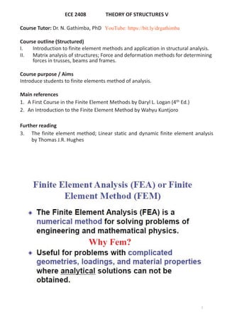
- 1. ECE 2408 THEORY OF STRUCTURES V Course Tutor: Dr. N. Gathimba, PhD Course outline (Structured) I. Introduction to finite element methods and application in structural analysis. II. Matrix analysis of structures; Force and deformation methods for determining forces in trusses, beams and frames. Course purpose / Aims Introduce students to finite elements method of analysis. Main references 1. A First Course in the Finite Element Methods by Daryl L. Logan (4th Ed.) 2. An Introduction to the Finite Element Method by Wahyu Kuntjoro Further reading 3. The finite element method; Linear static and dynamic finite element analysis by Thomas J.R. Hughes Why Fem? 2 YouTube: https://bit.ly/drgathimba
- 2. Analytical methods FEA methods (a numerical method) x Analytical solutions are those given by a mathematical expression that yields the values of the desired unknown quantities at any location in a body and are thus valid for an infinite number of locations in the body x Analytical methods involve solving for entire system in one operation. (solution of set(s) of ODE’s or PDE’s x Stress analysis for trusses, beams, and other simple structures are carried out based on dramatic simplification and idealization: – Mass concentrated at the center of gravity – Beam simplified as a line segment (same cross-section) x Design is based on the calculation results of the idealized structure & a large safety factor (1.5-3) given by experience. x FEA involving defining equations for each element and combining to obtain system solution. (simultaneous algebraic equations ) x FEM yields approximate values of the unknowns at discrete numbers of points in the continuum x Design geometry is a lot more complex; and the accuracy requirement is a lot higher. We need – To understand the physical behaviours of a complex object (strength, heat transfer capability, fluid flow, etc.) – To predict the performance and behaviour of the design; to calculate the safety margin; and to identify the weakness of the design accurately; and – To identify the optimal design with confidence FEA is therefore an approximation technique FEM Vs. Analytical Methods 3 This course will limit discussion to structural problems. 4
- 3. Role of Computers in FEM • FEM describes a complicated structures, resulting into large number of algebraic equations making the method extremely difficult to use. • However, with the advent of the computer, the solution of thousands of equations in a matter of minutes became possible. • The development of the computer resulted in the writing of computational programs. • Examples of special-purpose and general-purpose programs which can handle various complicated structural (and non structural) problems include Algor, Abaqus, ADINA, ANSYS, COSMOS/M, DIANA, SAP2000 etc. • To use the computer, the analyst, having defined the finite element model, inputs the information into the computer. • This information may include the position of the element nodal coordinates, the manner in which elements are connected, the material properties of the elements, the applied loads, boundary conditions, or constraints, and the kind of analysis to be performed. • The computer then uses this information to generate and solve the equations necessary to carry out the analysis. 5 Advantages of the Finite Element Method This method has a number of advantages that have made it very popular. • Model irregularly shaped bodies quite easily • Handle general load conditions without difficulty • Model bodies composed of several different materials because the element equations are evaluated individually • Handle unlimited numbers and kinds of boundary conditions • Vary the size of the elements to make it possible to use small elements where necessary • Alter the finite element model relatively easily and cheaply • Include dynamic effects • Handle nonlinear behaviour existing with large deformations and nonlinear materials The finite element method of structural analysis enables the designer to detect stress, vibration, and thermal problems during the design process and to evaluate design changes before the construction of a possible prototype. Thus confidence in the acceptability of the prototype is enhanced. Moreover, if used properly, the method can reduce the number of prototypes that d t b b ilt 6
- 4. 7 8
- 5. 9 FEM: EQUATIONS GENERATION I. Direct approaches a) Force, or flexibility, method, uses internal forces as the unknowns of the problem. First the equilibrium equations are used. Then necessary additional equations are found by introducing compatibility equations. The result is a set of algebraic equations for determining the redundant or unknown forces. b) Displacement, or stiffness, method, assumes the displacements of the nodes as the unknowns of the problem. For instance, compatibility conditions requiring that elements connected at a common node, along a common edge, or on a common surface before loading remain connected at that node, edge, or surface after deformation takes place are initially satisfied. Then the governing equations are expressed in terms of nodal displacements using the equations of equilibrium and an applicable law relating forces to displacements. • These two direct approaches result in different unknowns (forces or displacements) in the analysis and different matrices associated with their formulations (flexibilities or stiffnesses). It has been shown that, for computational purposes, the displacement (or stiffness) method is more desirable because its formulation is simpler for most structural analysis problems. Furthermore, a vast majority of general-purpose finite element programs have incorporated the displacement formulation for solving structural problems. Consequently, only the displacement method will be used throughout this course. 10
- 6. II. Variational Methods • These methods apply to both structural and non structural problems. The variational method includes a number of principles. a) Minimum potential energy principle is relatively easy to comprehend and is often introduced in basic mechanics courses and is the one that applies to materials behaving in a linear-elastic manner. b) Principle of virtual work is another variational principle often used to derive the governing equations. This principle applies more generally to materials that behave in a linear-elastic fashion, as well as those that behave in a nonlinear fashion. 11 FEM General Steps – Direct Stiffness (displacement) Method • Step 1 Discretization and Selection of the Element Types 9 dividing the body into an equivalent system of finite elements with associated nodes and choosing the most appropriate element type to model most closely the actual physical behaviour. • Step 2 Select a Displacement Function 9 The functions are expressed in terms of the nodal unknowns (in the two-dimensional problem, in terms of an x and a y component). • Step 3 Define the Strain= Displacement and Stress=Strain Relationships 9 In the case of one-dimensional deformation, say, in the x direction, we have strain related to displacement by 9 Stresses must be related to the strains through the stress/strain law— generally called the constitutive law e.g Hookes law • Step 4 Derive the Element Stiffness Matrix and Equations 9 Various methods for developing elemental stiffness matrices are: • Direct Equilibrium Method (Most widely used in this course) • Work or Energy Methods • Method of weighted residuals 12
- 7. 9 These equations are written conveniently in matrix form as 9 Or in a more compact form as • Step 5 Assemble the Element Equations to Obtain the Global and Introduce Boundary Conditions • Direct stiffness method employs the concept of continuity, or compatibility, which requires that the structure remain together and that no tears occur anywhere within the structure. The final assembled or global equation written in matrix form is ese equations are written conveniently in m m as Where ሼ݂ሽ is the vector of element nodal forces, ሾ݇ሿ is the element stiffness matrix (normally square and symmetric), and ሼ݀ሽ is the vector of unknown element nodal degrees of freedom or generalized displacements, n. Here generalized displacements may include such quantities as actual displacements, slopes, or even curvatures. 13 • Step 6 Solve for the Unknown Degrees of Freedom (or Generalized Displacements) 9 Equation (5), modified to account for the boundary conditions, is a set of simultaneous algebraic equations that can be written in expanded matrix form as where ሼܨሽ is the vector of global nodal forces, ሾܭሿ is the structure global or total stiffness matrix, (for most problems, the global stiffness matrix is square and symmetric) and ሼ݀ሽ is now the vector of known and unknown structure nodal degrees of freedom or generalized displacements. It can be shown that at this stage, the global stiffness matrix ሾܭሿ is a singular matrix because its determinant is equal to zero. To remove this singularity problem, we must invoke certain boundary conditions (or constraints or supports) so that the structure remains in place instead of moving as a rigid body. It is important to note that invoking boundary or support conditions results in a modification of the global Eq. (5). Also applied known loads have been accounted for in the global force matrix ሼܨሽ 5), modified to account for the boundary cond ous algebraic equations that can be written in Where now n is the structure total number of unknown nodal degrees of freedom. These equations can be solved for the ݀ܵ by using an elimination method (such as Gauss’s method) or any other method. The ݀ܵ are called the primary unknowns, because they are the first quantities determined using the stiffness (or displacement) finite element method. 14
- 8. • Step 7 Solve for the Element Strains and Stresses 9 For the structural stress-analysis problem, important secondary quantities of strain and stress (or moment and shear force) can be obtained because they can be directly expressed in terms of the displacements determined in step 6. Typical relationships between strain and displacement and between stress and strain— such as Eqs. (1) and (2) for one-dimensional stress given in step 3— can be used. • Step 8 Interpret the Results 9 The final goal is to interpret and analyze the results for use in the design/analysis process. Determination of locations in the structure where large deformations and large stresses occur is generally important in making design/analysis decisions. Postprocessor computer programs help the user to interpret the results by displaying them in graphical form. Practice: Students to revisit their notes on Matrices in preparation for the next lesson! ¾ Types of matrices (Null, unit, identity, singular, etc), matrix operation (addition/subtraction/division/multiplication), determinant of matrices, Transpose, inverse, solution of simultaneous equation by matrix method, etc 15