SlideShare uma empresa Scribd logo
1 de 21
Baixar para ler offline
Lecture slides by Kevin Wayne

Copyright © 2005 Pearson-Addison Wesley

http://www.cs.princeton.edu/~wayne/kleinberg-tardos
Last updated on 2/25/20 4:16 PM
4. GREEDY ALGORITHMS II
‣ Dijkstra′s algorithm
‣ minimum spanning trees
‣ Prim, Kruskal, Boruvka
‣ single-link clustering
‣ min-cost arborescences
4. GREEDY ALGORITHMS II
‣ Dijkstra′s algorithm
‣ minimum spanning trees
‣ Prim, Kruskal, Boruvka
‣ single-link clustering
‣ min-cost arborescences
SECTION 4.4
Single-pair shortest path problem
Problem. Given a digraph G = (V, E), edge lengths ℓe ≥ 0, source s ∈ V,
and destination t ∈ V, find a shortest directed path from s to t.
3
7
1 3
source s
6
8
5
7
5
4
15
3
12
20
13
9
destination t
length of path = 9 + 4 + 1 + 11 = 25
0
4
5
2
6
9
4
1
11
Single-source shortest paths problem
Problem. Given a digraph G = (V, E), edge lengths ℓe ≥ 0, source s ∈ V,
find a shortest directed path from s to every node.
4
7
1 3
source s
6
8
5
7
5
4
15
3
12
20
13
9
shortest-paths tree
4
5
2
6
4
1
11
9
0
Suppose that you change the length of every edge of G as follows.

For which is every shortest path in G a shortest path in G′? 

A. Add 17.
B. Multiply by 17.
C. Either A or B.
D. Neither A nor B.
5
Shortest paths: quiz 1
s t
1 2 3
7
24
—
19
—
18
—
20
—
Shortest paths: quiz 2
Which variant in car GPS?
A. Single source: from one node s to every other node.
B. Single sink: from every node to one node t.
C. Source–sink: from one node s to another node t.
D. All pairs: between all pairs of nodes.
6
Shortest path applications
・PERT/CPM.
・Map routing.
・Seam carving.
・Robot navigation.
・Texture mapping.
・Typesetting in LaTeX.
・Urban traffic planning.
・Telemarketer operator scheduling.
・Routing of telecommunications messages.
・Network routing protocols (OSPF, BGP, RIP).
・Optimal truck routing through given traffic congestion pattern.
7
Network Flows: Theory, Algorithms, and Applications,
by Ahuja, Magnanti, and Orlin, Prentice Hall, 1993.
Dijkstra′s algorithm (for single-source shortest paths problem)
Greedy approach. Maintain a set of explored nodes S for which
algorithm has determined d[u] = length of a shortest s↝u path.
・Initialize S ← { s }, d[s] ← 0.
・Repeatedly choose unexplored node v ∉ S which minimizes
8
s
v
u
S
d[u]
the length of a shortest path from s
to some node u in explored part S,
followed by a single edge e = (u, v)
(v) = min
e = (u,v) : u S
d[u] + e
ℓe
Greedy approach. Maintain a set of explored nodes S for which
algorithm has determined d[u] = length of a shortest s↝u path.
・Initialize S ← { s }, d[s] ← 0.
・Repeatedly choose unexplored node v ∉ S which minimizes
add v to S, and set d[v] ← π(v).
・To recover path, set pred[v] ← e that achieves min.
Dijkstra′s algorithm (for single-source shortest paths problem)
9
s
v
u
S
d[u]
d[v]
(v) = min
e = (u,v) : u S
d[u] + e
the length of a shortest path from s
to some node u in explored part S,
followed by a single edge e = (u, v)
ℓe
Invariant. For each node u ∈ S : d[u] = length of a shortest s↝u path.
Pf. [ by induction on ⎜S⎟ ]
Base case: ⎜S⎟ = 1 is easy since S = { s } and d[s] = 0.
Inductive hypothesis: Assume true for ⎜S⎟ ≥ 1.
・Let v be next node added to S, and let (u, v) be the final edge.
・A shortest s↝u path plus (u, v) is an s↝v path of length π(v).
・Consider any other s↝v path P. We show that it is no shorter than π(v).
・Let e = (x, y) be the first edge in P that leaves S,
and let Pʹ be the subpath from s to x.
・The length of P is already ≥ π (v) as soon
as it reaches y:
S
s
Dijkstra′s algorithm: proof of correctness
10
ℓ(P) ≥ ℓ(Pʹ) + ℓe
non-negative
lengths
v
u
y
P
x
Dijkstra chose v
instead of y
≥ π (v)
definition
of π(y)
≥ π (y)
inductive
hypothesis
≥ d[x] + ℓe ▪
Pʹ e
Dijkstra′s algorithm: efficient implementation
Critical optimization 1. For each unexplored node v ∉ S :
explicitly maintain π[v] instead of computing directly from definition
・For each v ∉ S : π(v) can only decrease (because set S increases).
・More specifically, suppose u is added to S and there is an edge e = (u, v)
leaving u. Then, it suffices to update:
Critical optimization 2. Use a min-oriented priority queue (PQ)
to choose an unexplored node that minimizes π[v].
11
π[v] ← min { π[v], π[u] + ℓe) }
(v) = min
e = (u,v) : u S
d[u] + e
recall: for each u ∈ S,
π[u] = d[u] = length of shortest s↝u path
Dijkstra’s algorithm: efficient implementation
Implementation.
・Algorithm maintains π[v] for each node v.
・Priority queue stores unexplored nodes, using π[⋅] as priorities.
・Once u is deleted from the PQ, π[u] = length of a shortest s↝u path.
12
DIJKSTRA (V, E, ℓ, s)
_________________________________________________________________________________________________________________________________________________________________________________________________________________________________________________________________________________________________________________________________________________________________________________________________________________________________________________________________________________________________________________________________________________________________________________________________________________________________________________________________________________________________________________________________________________________________________________________________________________________________________________________________________________________________________________________________________________________________________________________________________________________________________________________________________________________________________________________________________________________________________________________________________________________________________________________
FOREACH v ≠ s : π[v] ← ∞, pred[v] ← null; π[s] ← 0.
Create an empty priority queue pq.
FOREACH v ∈ V : INSERT(pq, v, π[v]).
WHILE (IS-NOT-EMPTY(pq))
u ← DEL-MIN(pq).
FOREACH edge e = (u, v) ∈ E leaving u:
IF (π[v] > π[u] + ℓe)
DECREASE-KEY(pq, v, π[u] + ℓe).
π[v] ← π[u] + ℓe ; pred[v] ← e.
Dijkstra′s algorithm: which priority queue?
Performance. Depends on PQ: n INSERT, n DELETE-MIN, ≤ m DECREASE-KEY.
・Array implementation optimal for dense graphs.
・Binary heap much faster for sparse graphs.
・4-way heap worth the trouble in performance-critical situations.
13
priority queue INSERT DELETE-MIN DECREASE-KEY total
node-indexed array
(A[i] = priority of i)
O(1) O(n) O(1) O(n2
)
binary heap O(log n) O(log n) O(log n) O(m log n)
d-way heap

(Johnson 1975)
O(d logd n) O(d logd n) O(logd n) O(m logm/n n)
Fibonacci heap

(Fredman–Tarjan 1984)
O(1) O(log n) † O(1) † O(m + n log n)
integer priority queue

(Thorup 2004)
O(1) O(log log n) O(1) O(m + n log log n)
† amortized
Θ(n2
) edges
Θ(n) edges
assumes m ≥ n
How to solve the the single-source shortest paths problem in
undirected graphs with positive edge lengths? 

A. Replace each undirected edge with two antiparallel edges of same
length. Run Dijkstra’s algorithm in the resulting digraph.
B. Modify Dijkstra’s algorithms so that when it processes node u,

it consider all edges incident to u (instead of edges leaving u).
C. Either A or B.
D. Neither A nor B.
14
Shortest paths: quiz 3
Theorem. [Thorup 1999] Can solve single-source shortest paths problem
in undirected graphs with positive integer edge lengths in O(m) time.
Remark. Does not explore nodes in increasing order of distance from s.
15
Shortest paths: quiz 3 Extensions of Dijkstra’s algorithm
Dijkstra’s algorithm and proof extend to several related problems:
・Shortest paths in undirected graphs: π[v] ≤ π[u] + ℓ(u, v).
・Maximum capacity paths: π[v] ≥ min { π[u], c(u, v) }.
・Maximum reliability paths: π[v] ≥ π[u] 𐄂 γ(u, v) .
・…
Key algebraic structure. Closed semiring (min-plus, bottleneck, Viterbi, …).
16
s
v
u
S
π[u]
ℓe
Fun with Semirings
A functional pearl on the abuse of linear algebra
Stephen Dolan
Computer Laboratory, University of Cambridge
stephen.dolan@cl.cam.ac.uk
Abstract
Describing a problem using classical linear algebra is a very well-
known problem-solving technique. If your question can be formu-
lated as a question about real or complex matrices, then the answer
can often be found by standard techniques.
It’s less well-known that very similar techniques still apply
where instead of real or complex numbers we have a closed semir-
ing, which is a structure with some analogue of addition and multi-
plication that need not support subtraction or division.
We define a typeclass in Haskell for describing closed semir-
ings, and implement a few functions for manipulating matrices and
polynomials over them. We then show how these functions can
be used to calculate transitive closures, find shortest or longest
or widest paths in a graph, analyse the data flow of imperative
programs, optimally pack knapsacks, and perform discrete event
simulations, all by just providing an appropriate underlying closed
semiring.
Categories and Subject Descriptors D.1.1 [Programming Tech-
niques]: Applicative (Functional) Programming; G.2.2 [Discrete
Mathematics]: Graph Theory—graph algorithms
Keywords closed semirings; transitive closure; linear systems;
shortest paths
1. Introduction
Linear algebra provides an incredibly powerful problem-solving
toolbox. A great many problems in computer graphics and vision,
machine learning, signal processing and many other areas can be
solved by simply expressing the problem as a system of linear
equations and solving using standard techniques.
Linear algebra is defined abstractly in terms of fields, of which
the real and complex numbers are the most familiar examples.
Fields are sets equipped with some notion of addition and multi-
plication as well as negation and reciprocals.
Many discrete mathematical structures commonly encountered
in computer science do not have sensible notions of negation.
Booleans, sets, graphs, regular expressions, imperative programs,
datatypes and various other structures can all be given natural no-
tions of product (interpreted variously as intersection, sequencing
or conjunction) and sum (union, choice or disjunction), but gener-
ally lack negation or reciprocals.
Such structures, having addition and multiplication (which dis-
tribute in the usual way) but not in general negation or reciprocals,
are called semirings. Many structures specifying sequential actions
can be thought of as semirings, with multiplication as sequencing
and addition as choice. The distributive law then states, intuitively,
a followed by a choice between b and c is the same as a choice
between a followed by b and a followed by c.
Plain semirings are a very weak structure. We can find many
examples of them in the wild, but unlike fields which provide
the toolbox of linear algebra, there isn’t much we can do with
something knowing only that it is a semiring.
However, we can build some useful tools by introducing the
closed semiring, which is a semiring equipped with an extra opera-
tion called closure. With the intuition of multiplication as sequenc-
ing and addition as choice, closure can be interpreted as iteration.
As we see in the following sections, it is possible to use something
akin to Gaussian elimination on an arbitrary closed semiring, giv-
ing us a means of solving certain “linear” equations over any struc-
ture with suitable notions of sequencing, choice and iteration. First,
though, we need to define the notion of semiring more precisely.
2. Semirings
We define a semiring formally as consisting of a set R, two distin-
guished elements of R named 0 and 1, and two binary operations
+ and ·, satisfying the following relations for any a, b, c 2 R:
a + b = b + a
a + (b + c) = (a + b) + c
a + 0 = a
a · (b · c) = (a · b) · c
a · 0 = 0 · a = 0
a · 1 = 1 · a = a
a · (b + c) = a · b + a · c
(a + b) · c = a · c + b · c
We often write a · b as ab, and a · a · a as a3
.
Our focus will be on closed semirings [12], which are semir-
ings with an additional operation called closure (denoted ⇤
) which
satisfies the axiom:
a⇤
= 1 + a · a⇤
= 1 + a⇤
· a
If we have an affine map x 7! ax + b in some closed semiring,
then x = a⇤
b is a fixpoint, since a⇤
b = (aa⇤
+ 1)b = a(a⇤
b) + b.
So, a closed semiring can also be thought of as a semiring where
affine maps have fixpoints.
Fun with Semirings
A functional pearl on the abuse of linear algebra
Stephen Dolan
Computer Laboratory, University of Cambridge
stephen.dolan@cl.cam.ac.uk
Abstract
Describing a problem using classical linear algebra is a very well-
known problem-solving technique. If your question can be formu-
lated as a question about real or complex matrices, then the answer
can often be found by standard techniques.
It’s less well-known that very similar techniques still apply
where instead of real or complex numbers we have a closed semir-
ing, which is a structure with some analogue of addition and multi-
plication that need not support subtraction or division.
We define a typeclass in Haskell for describing closed semir-
ings, and implement a few functions for manipulating matrices and
polynomials over them. We then show how these functions can
be used to calculate transitive closures, find shortest or longest
or widest paths in a graph, analyse the data flow of imperative
programs, optimally pack knapsacks, and perform discrete event
simulations, all by just providing an appropriate underlying closed
semiring.
Categories and Subject Descriptors D.1.1 [Programming Tech-
niques]: Applicative (Functional) Programming; G.2.2 [Discrete
Mathematics]: Graph Theory—graph algorithms
Keywords closed semirings; transitive closure; linear systems;
shortest paths
1. Introduction
Linear algebra provides an incredibly powerful problem-solving
toolbox. A great many problems in computer graphics and vision,
machine learning, signal processing and many other areas can be
solved by simply expressing the problem as a system of linear
equations and solving using standard techniques.
Linear algebra is defined abstractly in terms of fields, of which
the real and complex numbers are the most familiar examples.
Fields are sets equipped with some notion of addition and multi-
plication as well as negation and reciprocals.
Many discrete mathematical structures commonly encountered
in computer science do not have sensible notions of negation.
Booleans, sets, graphs, regular expressions, imperative programs,
datatypes and various other structures can all be given natural no-
tions of product (interpreted variously as intersection, sequencing
[Copyright notice will appear here once ’preprint’ option is removed.]
or conjunction) and sum (union, choice or disjunction), but gener-
ally lack negation or reciprocals.
Such structures, having addition and multiplication (which dis-
tribute in the usual way) but not in general negation or reciprocals,
are called semirings. Many structures specifying sequential actions
can be thought of as semirings, with multiplication as sequencing
and addition as choice. The distributive law then states, intuitively,
a followed by a choice between b and c is the same as a choice
between a followed by b and a followed by c.
Plain semirings are a very weak structure. We can find many
examples of them in the wild, but unlike fields which provide
the toolbox of linear algebra, there isn’t much we can do with
something knowing only that it is a semiring.
However, we can build some useful tools by introducing the
closed semiring, which is a semiring equipped with an extra opera-
tion called closure. With the intuition of multiplication as sequenc-
ing and addition as choice, closure can be interpreted as iteration.
As we see in the following sections, it is possible to use something
akin to Gaussian elimination on an arbitrary closed semiring, giv-
ing us a means of solving certain “linear” equations over any struc-
ture with suitable notions of sequencing, choice and iteration. First,
though, we need to define the notion of semiring more precisely.
2. Semirings
We define a semiring formally as consisting of a set R, two distin-
guished elements of R named 0 and 1, and two binary operations
+ and ·, satisfying the following relations for any a, b, c 2 R:
a + b = b + a
a + (b + c) = (a + b) + c
a + 0 = a
a · (b · c) = (a · b) · c
a · 0 = 0 · a = 0
a · 1 = 1 · a = a
a · (b + c) = a · b + a · c
(a + b) · c = a · c + b · c
We often write a · b as ab, and a · a · a as a3
.
Our focus will be on closed semirings [12], which are semir-
ings with an additional operation called closure (denoted ⇤
) which
satisfies the axiom:
a⇤
= 1 + a · a⇤
= 1 + a⇤
· a
If we have an affine map x 7! ax + b in some closed semiring,
then x = a⇤
b is a fixpoint, since a⇤
b = (aa⇤
+ 1)b = a(a⇤
b) + b.
So, a closed semiring can also be thought of as a semiring where
affine maps have fixpoints.
The definition of a semiring translates neatly to Haskell:
1 2013/7/17
17
GOOGLE’S FOO.BAR CHALLENGE
You have maps of parts of the space station, each starting at a prison exit
and ending at the door to an escape pod. The map is represented as a
matrix of 0s and 1s, where 0s are passable space and 1s are impassable
walls. The door out of the prison is at the top left (0, 0) and the door into
an escape pod is at the bottom right (w−1, h−1).
Write a function that generates the length of a shortest path from the
prison door to the escape pod, where you are allowed to remove one wall
as part of your remodeling plans.
s
t
Edsger Dijkstra
19
“ What’s the shortest way to travel from Rotterdam to Groningen?
It is the algorithm for the shortest path, which I designed in
about 20 minutes. One morning I was shopping in Amsterdam
with my young fiancée, and tired, we sat down on the café
terrace to drink a cup of coffee and I was just thinking about
whether I could do this, and I then designed the algorithm for
the shortest path. ” — Edsger Dijsktra
The moral implications of implementing shortest-path algorithms
20
https://www.facebook.com/pg/npcompleteteens
4. GREEDY ALGORITHMS II
‣ Dijkstra′s algorithm
‣ minimum spanning trees
‣ Prim, Kruskal, Boruvka
‣ single-link clustering
‣ min-cost arborescences
SECTION 6.1
Def. A path is a sequence of edges which connects a sequence of nodes.
Def. A cycle is a path with no repeated nodes or edges other than the
starting and ending nodes.
Cycles
22
1
2 3
4
8
5
6
7
cycle C = { (1, 2), (2, 3), (3, 4), (4, 5), (5, 6), (6, 1) }
1 6
2 3
4
5
path P = { (1, 2), (2, 3), (3, 4), (4, 5), (5, 6) }
4
8
5
Cuts
Def. A cut is a partition of the nodes into two nonempty subsets S and V – S.
Def. The cutset of a cut S is the set of edges with exactly one endpoint in S.
23
1
2 3
4
8
5
6
7
cutset D = { (3, 4), (3, 5), (5, 6), (5, 7), (8, 7) }
1
2 3
6
7
cut S = { 4, 5, 8 }
Minimum spanning trees: quiz 1
Consider the cut S = { 1, 4, 6, 7 }. Which edge is in the cutset of S?
A. S is not a cut (not connected)
B. 1–7
C. 5–7
D. 2–3
24
5
4
7
1
3
8
2
6
Minimum spanning trees: quiz 2
Let C be a cycle and let D be a cutset. How many edges do C and D
have in common? Choose the best answer.
A. 0
B. 2
C. not 1
D. an even number
25
Cycle–cut intersection
Proposition. A cycle and a cutset intersect in an even number of edges.
26
1
2 3
4
8
5
6
7
cutset D = { (3, 4), (3, 5), (5, 6), (5, 7), (8, 7) }
intersection C ∩ D = { (3, 4), (5, 6) }
cycle C = { (1, 2), (2, 3), (3, 4), (4, 5), (5, 6), (6, 1) }
Cycle–cut intersection
Proposition. A cycle and a cutset intersect in an even number of edges.
Pf. [by picture]
27
cycle C
S
Def. Let H = (V, T) be a subgraph of an undirected graph G = (V, E).
H is a spanning tree of G if H is both acyclic and connected.
Spanning tree definition
28
graph G = (V, E)
spanning tree H = (V, T)
Minimum spanning trees: quiz 3
Which of the following properties are true for all spanning trees H?
A. Contains exactly ⎜V⎟ – 1 edges.
B. The removal of any edge disconnects it.
C. The addition of any edge creates a cycle.
D. All of the above.
29
graph G = (V, E)
spanning tree H = (V, T)
Spanning tree properties
Proposition. Let H = (V, T) be a subgraph of an undirected graph G = (V, E).
Then, the following are equivalent:
・H is a spanning tree of G.
・H is acyclic and connected.
・H is connected and has ⎜V⎟ – 1 edges.
・H is acyclic and has ⎜V⎟ – 1 edges.
・H is minimally connected: removal of any edge disconnects it.
・H is maximally acyclic: addition of any edge creates a cycle.
30
graph G = (V, E)
spanning tree H = (V, T) 31
https://maps.roadtrippers.com/places/46955/photos/374771356
A tree containing a cycle
Minimum spanning tree (MST)
Def. Given a connected, undirected graph G = (V, E) with edge costs ce,
a minimum spanning tree (V, T) is a spanning tree of G such that the sum
of the edge costs in T is minimized.
Cayley’s theorem. The complete graph on n nodes has nn–2 spanning trees.
32
can’t solve by brute force
MST cost = 50 = 4 + 6 + 8 + 5 + 11 + 9 + 7
16
4
6 23
10
21
14
24
18
9
7
11
5
8
Suppose that you change the cost of every edge in G as follows.

For which is every MST in G an MST in G′ (and vice versa)?

Assume c(e) > 0 for each e.

A. cʹ(e) = c(e) + 17.
B. cʹ(e) = 17 𐄂 c(e).
C. cʹ(e) = log17 c(e).
D. All of the above.
33
Minimum spanning trees: quiz 4
Applications
MST is fundamental problem with diverse applications.
・Dithering.
・Cluster analysis.
・Max bottleneck paths.
・Real-time face verification.
・LDPC codes for error correction.
・Image registration with Renyi entropy.
・Find road networks in satellite and aerial imagery.
・Model locality of particle interactions in turbulent fluid flows.
・Reducing data storage in sequencing amino acids in a protein.
・Autoconfig protocol for Ethernet bridging to avoid cycles in a network.
・Approximation algorithms for NP-hard problems (e.g., TSP, Steiner tree).
・Network design (communication, electrical, hydraulic, computer, road).
34
Network Flows: Theory, Algorithms, and Applications,
by Ahuja, Magnanti, and Orlin, Prentice Hall, 1993.
Fundamental cycle. Let H = (V, T) be a spanning tree of G = (V, E).
・For any non tree-edge e ∈ E : T ∪ { e } contains a unique cycle, say C.
・For any edge f ∈ C : (V, T ∪ { e } – { f }) is a spanning tree.
Observation. If ce < cf, then (V, T) is not an MST.
Fundamental cycle
35
e
f
graph G = (V, E)
spanning tree H = (V, T)
Fundamental cutset
Fundamental cutset. Let H = (V, T) be a spanning tree of G = (V, E).
・For any tree edge f ∈ T : (V, T – { f }) has two connected components.
・Let D denote corresponding cutset.
・For any edge e ∈ D : (V, T – { f } ∪ { e }) is a spanning tree.
Observation. If ce < cf, then (V, T) is not an MST. 36
e
f
graph G = (V, E)
spanning tree H = (V, T)
The greedy algorithm
Red rule.
・Let C be a cycle with no red edges.
・Select an uncolored edge of C of max cost and color it red.
Blue rule.
・Let D be a cutset with no blue edges.
・Select an uncolored edge in D of min cost and color it blue.
Greedy algorithm.
・Apply the red and blue rules (nondeterministically!) until all edges
are colored. The blue edges form an MST.
・Note: can stop once n – 1 edges colored blue.
37
Greedy algorithm: proof of correctness
Color invariant. There exists an MST (V, T*) containing every blue edge
and no red edge.
Pf. [ by induction on number of iterations ]
Base case. No edges colored ⇒ every MST satisfies invariant.
38
Greedy algorithm: proof of correctness
Color invariant. There exists an MST (V, T*) containing every blue edge
and no red edge.
Pf. [ by induction on number of iterations ]
Induction step (blue rule). Suppose color invariant true before blue rule.
・let D be chosen cutset, and let f be edge colored blue.
・if f ∈ T*, then T* still satisfies invariant.
・Otherwise, consider fundamental cycle C by adding f to T*.
・let e ∈ C be another edge in D.
・e is uncolored and ce ≥ cf since
- e ∈ T* ⇒ e not red
- blue rule ⇒ e not blue and ce ≥ cf
・Thus, T* ∪ { f } – { e } satisfies invariant.
39
f
T*
e
cut
Greedy algorithm: proof of correctness
Color invariant. There exists an MST (V, T*) containing every blue edge
and no red edge.
Pf. [ by induction on number of iterations ]
Induction step (red rule). Suppose color invariant true before red rule.
・let C be chosen cycle, and let e be edge colored red.
・if e ∉ T*, then T* still satisfies invariant.
・Otherwise, consider fundamental cutset D by deleting e from T*.
・let f ∈ D be another edge in C.
・f is uncolored and ce ≥ cf since
- f ∉ T* ⇒ f not blue
- red rule ⇒ f not red and ce ≥ cf
・Thus, T* ∪ { f } – { e } satisfies invariant. ▪
40
f
T*
e
cut
Greedy algorithm: proof of correctness
Theorem. The greedy algorithm terminates. Blue edges form an MST.
Pf. We need to show that either the red or blue rule (or both) applies.
・Suppose edge e is left uncolored.
・Blue edges form a forest.
・Case 1: both endpoints of e are in same blue tree.
⇒ apply red rule to cycle formed by adding e to blue forest.
41
Case 1
e
Greedy algorithm: proof of correctness
Theorem. The greedy algorithm terminates. Blue edges form an MST.
Pf. We need to show that either the red or blue rule (or both) applies.
・Suppose edge e is left uncolored.
・Blue edges form a forest.
・Case 1: both endpoints of e are in same blue tree.
⇒ apply red rule to cycle formed by adding e to blue forest.
・Case 2: both endpoints of e are in different blue trees.
⇒ apply blue rule to cutset induced by either of two blue trees. ▪
42
Case 2
e
4. GREEDY ALGORITHMS II
‣ Dijkstra′s algorithm
‣ minimum spanning trees
‣ Prim, Kruskal, Boruvka
‣ single-link clustering
‣ min-cost arborescences
SECTION 6.2
Prim′s algorithm
Initialize S = { s } for any node s, T = ∅.
Repeat n – 1 times:
・Add to T a min-cost edge with exactly one endpoint in S.
・Add the other endpoint to S.
Theorem. Prim’s algorithm computes an MST.
Pf. Special case of greedy algorithm (blue rule repeatedly applied to S). ▪
44
S
by construction, edges in
cutset are uncolored
Prim′s algorithm: implementation
Theorem. Prim’s algorithm can be implemented to run in O(m log n) time.
Pf. Implementation almost identical to Dijkstra’s algorithm.
45
PRIM (V, E, c)
_________________________________________________________________________________________________________________________________________________________________________________________________________________________________________________________________________________________________________________________________________________________________________________________________________________________________________________________________________________________________________________________________________________________________________________________________________________________________________________________________________________________________________________________________________________________________________________________________________________________________________________________________________________________________________________________________________________________________________________________________________________________________________________________________________________________________________________________________________________________________________________________________________________________________________________________
S ← ∅, T ← ∅.
s ← any node in V.
FOREACH v ≠ s : π[v] ← ∞, pred[v] ← null; π[s] ← 0.
Create an empty priority queue pq.
FOREACH v ∈ V : INSERT(pq, v, π[v]).
WHILE (IS-NOT-EMPTY(pq))
u ← DEL-MIN(pq).
S ← S ∪ { u }, T ← T ∪ { pred[u] }.
FOREACH edge e = (u, v) ∈ E with v ∉ S :
IF (ce < π[v])
DECREASE-KEY(pq, v, ce).
π[v] ← ce; pred[v] ← e.
π[v] = cost of cheapest
known edge between v and S
Kruskal′s algorithm
Consider edges in ascending order of cost:
・Add to tree unless it would create a cycle.
Theorem. Kruskal’s algorithm computes an MST.
Pf. Special case of greedy algorithm.
・Case 1: both endpoints of e in same blue tree.
⇒ color e red by applying red rule to unique cycle.
・Case 2: both endpoints of e in different blue trees.
⇒ color e blue by applying blue rule to cutset defined by either tree. ▪
46
e
all other edges in cycle are blue
no edge in cutset has smaller cost
(since Kruskal chose it first)
Kruskal′s algorithm: implementation
Theorem. Kruskal’s algorithm can be implemented to run in O(m log m) time.
・Sort edges by cost.
・Use union–find data structure to dynamically maintain connected
components.
47
KRUSKAL (V, E, c)
________________________________________________________________________________________________________________________________________________________________________________________________________________________________________________________________________________________________________________________________________________________________________________________________________________________________________________________________________________________________________________________________________________________________________________________________________________________________________________________________________________________________________________________________________________________________________________________________________________________________________________________________________________________________________________________________________________________________________________________________________________________________________________________________________________________________________________________________________________________________________________________________________________________________
SORT m edges by cost and renumber so that c(e1) ≤ c(e2) ≤ … ≤ c(em).
T ← ∅.
FOREACH v ∈ V : MAKE-SET(v).
FOR i = 1 TO m
(u, v) ← ei.
IF (FIND-SET(u) ≠ FIND-SET(v))
T ← T ∪ { ei }.
UNION(u, v).
RETURN T.
are u and v in
same component?
make u and v in
same component
Reverse-delete algorithm
Start with all edges in T and consider them in descending order of cost:
・Delete edge from T unless it would disconnect T.
Theorem. The reverse-delete algorithm computes an MST.
Pf. Special case of greedy algorithm.
・Case 1. [ deleting edge e does not disconnect T ]
⇒ apply red rule to cycle C formed by adding e to another path
in T between its two endpoints
・Case 2. [ deleting edge e disconnects T ]
⇒ apply blue rule to cutset D induced by either component ▪


Fact. [Thorup 2000] Can be implemented to run in O(m log n (log log n)3) time.
48
no edge in C is more expensive
(it would have already been considered and deleted)
e is the only remaining edge in the cutset
(all other edges in D must have been colored red / deleted)
Review: the greedy MST algorithm
Red rule.
・Let C be a cycle with no red edges.
・Select an uncolored edge of C of max cost and color it red.
Blue rule.
・Let D be a cutset with no blue edges.
・Select an uncolored edge in D of min cost and color it blue.
Greedy algorithm.
・Apply the red and blue rules (nondeterministically!) until all edges
are colored. The blue edges form an MST.
・Note: can stop once n – 1 edges colored blue.
Theorem. The greedy algorithm is correct.
Special cases. Prim, Kruskal, reverse-delete, …
49
Borůvka′s algorithm
Repeat until only one tree.
・Apply blue rule to cutset corresponding to each blue tree.
・Color all selected edges blue.
Theorem. Borůvka’s algorithm computes the MST.
Pf. Special case of greedy algorithm (repeatedly apply blue rule). ▪
50
7 11
5
8 12
13
assume edge
costs are distinct
Borůvka′s algorithm: implementation
Theorem. Borůvka’s algorithm can be implemented to run in O(m log n) time.
Pf.
・To implement a phase in O(m) time:
- compute connected components of blue edges
- for each edge (u, v) ∈ E, check if u and v are in different components;
if so, update each component’s best edge in cutset
・≤ log2 n phases since each phase (at least) halves total # components. ▪
51
7 11
5
8 12
13
Borůvka′s algorithm: implementation
Contraction version.
・After each phase, contract each blue tree to a single supernode.
・Delete self-loops and parallel edges (keeping only cheapest one).
・Borůvka phase becomes: take cheapest edge incident to each node.
Q. How to contract a set of edges? 52
2 3
5
4 6
1 8
3 4 2
9
7
5
6 3
4 6
1
8
3 2
9
7
5
6
2, 5
3
4 6
1
8
3 2
9
7
5
2, 5
graph G contract edge 2-5
delete self-loops and parallel edges
1 1
1
Problem. Given a graph G = (V, E) and a set of edges F, contract all edges
in F, removing any self-loops or parallel edges.
Goal. O(m + n) time.
CONTRACT A SET OF EDGES
53
graph G
contracted graph G′
CONTRACT A SET OF EDGES
Problem. Given a graph G = (V, E) and a set of edges F, contract all edges
in F, removing any self-loops or parallel edges.
Solution.
・Compute the nʹ connected components in (V, F).
・Suppose id[u] = i means node u is in connected component i.
・The contracted graph Gʹ has nʹ nodes.
・For each edge u–v ∈ E, add an edge i–j to Gʹ, where i = id[u] and j = id[v].
Removing self loops. Easy.
Removing parallel edges.
・Create a list of edges i–j with the convention that i < j.
・Sort the edges lexicographically via LSD radix sort.
・Add the edges to the graph Gʹ, removing parallel edges.
54
Theorem. Borůvka’s algorithm (contraction version) can be implemented to
run in O(n) time on planar graphs.
Pf.
・Each Borůvka phase takes O(n) time:
- Fact 1: m ≤ 3n for simple planar graphs.
- Fact 2: planar graphs remains planar after edge contractions/deletions.
・Number of nodes (at least) halves in each phase.
・Thus, overall running time ≤ cn + cn / 2 + cn / 4 + cn / 8 + … = O(n). ▪
Borůvka′s algorithm on planar graphs
55
planar K3,3 not planar
A hybrid algorithm
Borůvka–Prim algorithm.
・Run Borůvka (contraction version) for log2 log2 n phases.
・Run Prim on resulting, contracted graph.
Theorem. Borůvka–Prim computes an MST.
Pf. Special case of the greedy algorithm.
Theorem. Borůvka–Prim can be implemented to run in O(m log log n) time.
Pf.
・The log2 log2 n phases of Borůvka’s algorithm take O(m log log n) time;
resulting graph has ≤ n / log2 n nodes and ≤ m edges.
・Prim’s algorithm (using Fibonacci heaps) takes O(m + n) time on a
graph with n / log2 n nodes and m edges. ▪
56
O m +
n
log n
log
n
log n
Does a linear-time compare-based MST algorithm exist?
Theorem. [Fredman–Willard 1990] O(m) in word RAM model.
Theorem. [Dixon–Rauch–Tarjan 1992] O(m) MST verification algorithm.
Theorem. [Karger–Klein–Tarjan 1995] O(m) randomized MST algorithm. 57
deterministic compare-based MST algorithms
year worst case discovered by
1975 O(m log log n) Yao
1976 O(m log log n) Cheriton–Tarjan
1984 O(m log*n), O(m + n log n) Fredman–Tarjan
1986 O(m log (log* n)) Gabow–Galil–Spencer–Tarjan
1997 O(m α(n) log α(n)) Chazelle
2000 O(m α(n)) Chazelle
2002 asymptotically optimal Pettie–Ramachandran
20xx O(m)
n lg* n
(−∞, 1] 0
(1, 2] 1
(2, 4] 2
(4, 16] 3
(16, 216] 4
(216, 265536] 5
lg n =
0 n 1
1 + lg (lg n) n > 1
<latexit sha1_base64="HJFYyV8ahuzHjW6Ka99U33ko4ac=">AAACkXicbVFdaxNBFJ1s/ajrV1p98+ViUKpC2BWhraAEfRF8qWBsIRPD7OzdZOjs7DJztyQs+Yu++z/6WnGy2QeTeGGGw7nnfsyZpNTKURT97gR7t27fubt/L7z/4OGjx92Dwx+uqKzEoSx0YS8S4VArg0NSpPGitCjyRON5cvl5lT+/QutUYb7TosRxLqZGZUoK8tSkO+N6+vM1GPgQ8gSnytTSd3PLMIKXwAnnBDWoDJZewjVCDJyHMbyBpu7I32Be7Uo/roUcTdo2nHR7UT9qAnZB3IIea+NsctA55GkhqxwNSS2cG8VRSeNaWFJS4zLklcNSyEsxxZGHRuToxnVjyRJeeCaFrLD+GIKG/beiFrlzizzxylzQzG3nVuT/cqOKspNxrUxZERq5HpRVGqiAlb+QKouS9MIDIa3yu4KcCSsk+V/YmNL0LlFuvKSeV0bJIsUtVtOcrFi5GG97tguGb/un/ejbu97gpLVznz1jz9kRi9kxG7Av7IwNmWS/2DW7YX+Cp8H7YBB8WkuDTlvzhG1E8PUvXjrGCA==</latexit>
iterated logarithm function
MINIMUM BOTTLENECK SPANNING TREE
Problem. Given a connected graph G with positive edge costs, find a
spanning tree that minimizes the most expensive edge.
Goal. O(m log m) time or better.
58
minimum bottleneck spanning tree T (bottleneck = 9)
6 5
9
7
8 7 14
21
3
24
4 10 11
Note: not necessarily a MST
9
4. GREEDY ALGORITHMS II
‣ Dijkstra′s algorithm
‣ minimum spanning trees
‣ Prim, Kruskal, Boruvka
‣ single-link clustering
‣ min-cost arborescences
SECTION 4.7
Goal. Given a set U of n objects labeled p1, …, pn, partition into clusters so
that objects in different clusters are far apart.
Applications.
・Routing in mobile ad-hoc networks.
・Document categorization for web search.
・Similarity searching in medical image databases
・Cluster celestial objects into stars, quasars, galaxies.
・...
Clustering
outbreak of cholera deaths in London in 1850s (Nina Mishra)
62 4-clustering
k-clustering. Divide objects into k non-empty groups.
Distance function. Numeric value specifying “closeness” of two objects.
・d(pi, pj) = 0 iff pi = pj [ identity of indiscernibles ]
・d(pi, pj) ≥ 0 [ non-negativity ]
・d(pi, pj) = d(pj, pi) [ symmetry ]
Spacing. Min distance between any pair of points in different clusters.
Goal. Given an integer k, find a k-clustering of maximum spacing.
Clustering of maximum spacing
63
distance between
two clusters
min distance between
two closest clusters
Greedy clustering algorithm
“Well-known” algorithm in science literature for single-linkage k-clustering:
・Form a graph on the node set U, corresponding to n clusters.
・Find the closest pair of objects such that each object is in a different
cluster, and add an edge between them.
・Repeat n – k times (until there are exactly k clusters).
Key observation. This procedure is precisely Kruskal’s algorithm
(except we stop when there are k connected components).
Alternative. Find an MST and delete the k – 1 longest edges. 64
Greedy clustering algorithm: analysis
Theorem. Let C* denote the clustering C*
1, …, C*
k formed by deleting the
k – 1 longest edges of an MST. Then, C* is a k-clustering of max spacing.
Pf.
・Let C denote any other clustering C1, …, Ck.
・Let pi and pj be in the same cluster in C*, say C*
r , but different clusters
in C, say Cs and Ct.
・Some edge (p, q) on pi – pj path in C*
r spans two different clusters in C.
・Spacing of C* = length d* of the (k – 1)st longest edge in MST.
・Edge (p, q) has length ≤ d* since it was added by Kruskal.
・Spacing of C is ≤ d* since p and q are in different clusters. ▪
65
p q
pi
pj
Cs Ct
C*
r
edges left after deleting
k – 1 longest edges
from a MST
this is the edge
Kruskal would have
added next had
we not stopped it
Dendrogram of cancers in human
Tumors in similar tissues cluster together.
Reference: Botstein & Brown group
gene 1
gene n
gene expressed
gene not expressed
66
Which MST algorithm should you use for single-link clustering?

A. Kruskal (stop when there are k components).
B. Prim (delete k – 1 longest edges).
C. Either A or B.
D. Neither A nor B.
67
Minimum spanning trees: quiz 5
number of objects n
can be very large
4. GREEDY ALGORITHMS II
‣ Dijkstra′s algorithm
‣ minimum spanning trees
‣ Prim, Kruskal, Boruvka
‣ single-link clustering
‣ min-cost arborescences
SECTION 4.9
Arborescences
Def. Given a digraph G = (V, E) and a root r ∈ V, an arborescence (rooted at r)
is a subgraph T = (V, F) such that
・T is a spanning tree of G if we ignore the direction of edges.
・There is a (unique) directed path in T from r to each other node v ∈ V.
69
r
Which of the following are properties of arborescences rooted at r?

A. No directed cycles.
B. Exactly n − 1 edges.
C. For each v ≠ r : indegree(v) = 1.
D. All of the above.
70
Minimum spanning arborescence: quiz 1
r
Arborescences
Proposition. A subgraph T = (V, F) of G is an arborescence rooted at r iff
T has no directed cycles and each node v ≠ r has exactly one entering edge.
Pf.
⇒ If T is an arborescence, then no (directed) cycles and every node v ≠ r
has exactly one entering edge—the last edge on the unique r↝v path.
⇐ Suppose T has no cycles and each node v ≠ r has one entering edge.
・To construct an r↝v path, start at v and repeatedly follow edges in the
backward direction.
・Since T has no directed cycles, the process must terminate.
・It must terminate at r since r is the only node with no entering edge. ▪

71
Given a digraph G, how to find an arborescence rooted at r?

A. Breadth-first search from r.
B. Depth-first search from r.
C. Either A or B.
D. Neither A nor B.
72
Minimum spanning arborescence: quiz 2
r
Min-cost arborescence problem
Problem. Given a digraph G with a root node r and edge costs ce ≥ 0,
find an arborescence rooted at r of minimum cost.
Assumption 1. All nodes reachable from r.
Assumption 2. No edge enters r (safe to delete since they won’t help).
73
r
4
1
2
3
5
6
9
7
8
A min-cost arborescence must…

A. Include the cheapest edge.
B. Exclude the most expensive edge.
C. Be a shortest-paths tree from r.
D. None of the above.
74
Minimum spanning arborescence: quiz 3
r
8
3
4
6
10
12
A sufficient optimality condition
Property. For each node v ≠ r, choose a cheapest edge entering v
and let F* denote this set of n – 1 edges. If (V, F*) is an arborescence,
then it is a min-cost arborescence.
Pf. An arborescence needs exactly one edge entering each node v ≠ r
and (V, F*) is the cheapest way to make each of these choices. ▪
75
r
4
2
1
3
5
6
9
7
8
F* = thick black edges
A sufficient optimality condition
Property. For each node v ≠ r, choose a cheapest edge entering v
and let F* denote this set of n – 1 edges. If (V, F*) is an arborescence,
then it is a min-cost arborescence.
Note. F* may not be an arborescence (since it may have directed cycles).
76
r
4
1
2
3
5
6
9
7
8
F* = thick black edges
Reduced costs
Def. For each v ≠ r, let y(v) denote the min cost of any edge entering v.
Define the reduced cost of an edge (u, v) as cʹ(u, v) = c(u, v) – y(v) ≥ 0.
Observation. T is a min-cost arborescence in G using costs c iff
T is a min-cost arborescence in G using reduced costs cʹ.
Pf. For each v ≠ r : each arborescence has exactly one edge entering v. ▪
77
r
4
1
2
3
7
9 r
0
0
1
0
3
0
costs c reduced costs c′
1 9
4 3 y(v)
Intuition. Recall F* = set of cheapest edges entering v for each v ≠ r.
・Now, all edges in F* have 0 cost with respect to reduced costs cʹ(u, v).
・If F* does not contain a cycle, then it is a min-cost arborescence.
・If F* contains a cycle C, can afford to use as many edges in C as desired.
・Contract edges in C to a supernode (removing any self-loops).
・Recursively solve problem in contracted network Gʹ with costs cʹ(u, v).
Edmonds branching algorithm: intuition
78
r
0
3
4
1
0
0
0
4 0
0
7
1
0
F* = thick edges
Edmonds branching algorithm: intuition
Intuition. Recall F* = set of cheapest edges entering v for each v ≠ r.
・Now, all edges in F* have 0 cost with respect to reduced costs cʹ(u, v).
・If F* does not contain a cycle, then it is a min-cost arborescence.
・If F* contains a cycle C, can afford to use as many edges in C as desired.
・Contract edges in C to a supernode (removing any self-loops).
・Recursively solve problem in contracted network Gʹ with costs cʹ(u, v).
79
r
3
4
0
0
7
1
1 0
Edmonds branching algorithm
80
EDMONDS-BRANCHING (G, r , c)
_________________________________________________________________________________________________________________________________________________________________________________________________________________________________________________________________________________________________________________________________________________________________________________________________________________________________________________________________________________________________________________________________________________________________________________________________________________________________________________________________________________________________________________________________________________________________________________________________________________________________________________________________________________________________________________________________________________________________________________________________________________________________________________________________________________________________________________________________________________________________________________________________________________________________________________________________________________________________________________________________________________________________________________________________________________________________________________
FOREACH v ≠ r :
y(v) ← min cost of any edge entering v.
cʹ(u, v) ← cʹ(u, v) – y(v) for each edge (u, v) entering v.
FOREACH v ≠ r : choose one 0-cost edge entering v and let F*
be the resulting set of edges.
IF (F* forms an arborescence) RETURN T = (V, F*).
ELSE
C ← directed cycle in F*.
Contract C to a single supernode, yielding Gʹ = (Vʹ, Eʹ).
T ʹ ← EDMONDS-BRANCHING(Gʹ, r , cʹ).
Extend T ʹ to an arborescence T in G by adding all but one edge of C.
RETURN T.
_________________________________________________________________________________________________________________________________________________________________________________________________________________________________________________________________________________________________________________________________________________________________________________________________________________________________________________________________________________________________________________________________________________________________________________________________________________________________________________________________________________________________________________________________________________________________________________________________________________________________________________________________________________________________________________________________________________________________________________________________________________________________________________________________________________________________________________________________________________________________________________________________________________________________________________________________________________________________________________________________________________________________________________________________________________________________________________
Edmonds branching algorithm
Q. What could go wrong?
A. Contracting cycle C places extra constraint on arborescence.
・Min-cost arborescence in Gʹ must have exactly one edge entering
a node in C (since C is contracted to a single node)
・But min-cost arborescence in G might have several edges entering C.
81
b
a
r
cycle C
min-cost arborescence in G
Edmonds branching algorithm: key lemma
Lemma. Let C be a cycle in G containing only 0-cost edges. There exists a
min-cost arborescence T rooted at r that has exactly one edge entering C.
Pf.
Case 0. T has no edges entering C.
Since T is an arborescence, there is an r↝v path for each node v ⇒
at least one edge enters C. ※
Case 1. T has exactly one edge entering C.
T satisfies the lemma.
Case 2. T has two (or more) edges entering C.
We construct another min-cost arborescence T * that has exactly one edge
entering C.
82
Edmonds branching algorithm: key lemma
Case 2 construction of T *.
・Let (a, b) be an edge in T entering C that lies on a shortest path from r.
・We delete all edges of T that enter a node in C except (a, b).
・We add in all edges of C except the one that enters b.
b
83
a
r
cycle C
T
this path from r to C
uses only one node in C
T
Edmonds branching algorithm: key lemma
Case 2 construction of T *.
・Let (a, b) be an edge in T entering C that lies on a shortest path from r.
・We delete all edges of T that enter a node in C except (a, b).
・We add in all edges of C except the one that enters b.
Claim. T * is a min-cost arborescence.
・The cost of T * is at most that of T since we add only 0-cost edges.
・T * has exactly one edge entering each node v ≠ r.
・T * has no directed cycles.
(T had no cycles before; no cycles within C; now only (a, b) enters C)
b
84
b
a
T is an arborescence rooted at r
r
cycle C
T*
and the only path in T * to a
is the path from r to a
(since any path must follow
unique entering edge back to r)
this path from r to C
uses only one node in C
Edmonds branching algorithm: analysis
Theorem. [Chu–Liu 1965, Edmonds 1967] The greedy algorithm finds a
min-cost arborescence.
Pf. [ by strong induction on number of nodes ]
・If the edges of F* form an arborescence, then min-cost arborescence.
・Otherwise, we use reduced costs, which is equivalent.
・After contracting a 0-cost cycle C to obtain a smaller graph Gʹ,
the algorithm finds a min-cost arborescence T ʹ in Gʹ (by induction).
・Key lemma: there exists a min-cost arborescence T in G that
corresponds to T ʹ. ▪


Theorem. The greedy algorithm can be implemented to run in O(m n) time.
Pf.
・At most n contractions (since each reduces the number of nodes).
・Finding and contracting the cycle C takes O(m) time.
・Transforming T ʹ into T takes O(m) time. ▪
85
un-contracting cycle C,
remove all but one edge entering C,
taking all but one edge in C
Min-cost arborescence
Theorem. [Gabow–Galil–Spencer–Tarjan 1985] There exists an O(m + n log n)
time algorithm to compute a min-cost arborescence.
86

Mais conteúdo relacionado

Mais procurados

Algorithm Design and Complexity - Course 9
Algorithm Design and Complexity - Course 9Algorithm Design and Complexity - Course 9
Algorithm Design and Complexity - Course 9Traian Rebedea
 
Treewidth and Applications
Treewidth and ApplicationsTreewidth and Applications
Treewidth and ApplicationsASPAK2014
 
Bidimensionality
BidimensionalityBidimensionality
BidimensionalityASPAK2014
 
Algorithm Design and Complexity - Course 11
Algorithm Design and Complexity - Course 11Algorithm Design and Complexity - Course 11
Algorithm Design and Complexity - Course 11Traian Rebedea
 
Algorithm Design and Complexity - Course 7
Algorithm Design and Complexity - Course 7Algorithm Design and Complexity - Course 7
Algorithm Design and Complexity - Course 7Traian Rebedea
 
Important Cuts
Important CutsImportant Cuts
Important CutsASPAK2014
 
Hierarchical matrices for approximating large covariance matries and computin...
Hierarchical matrices for approximating large covariance matries and computin...Hierarchical matrices for approximating large covariance matries and computin...
Hierarchical matrices for approximating large covariance matries and computin...Alexander Litvinenko
 
Dijkstra's Algorithm
Dijkstra's AlgorithmDijkstra's Algorithm
Dijkstra's Algorithmguest862df4e
 
Tutorial of topological_data_analysis_part_1(basic)
Tutorial of topological_data_analysis_part_1(basic)Tutorial of topological_data_analysis_part_1(basic)
Tutorial of topological_data_analysis_part_1(basic)Ha Phuong
 

Mais procurados (19)

Chapter 24 aoa
Chapter 24 aoaChapter 24 aoa
Chapter 24 aoa
 
Algorithm Design and Complexity - Course 9
Algorithm Design and Complexity - Course 9Algorithm Design and Complexity - Course 9
Algorithm Design and Complexity - Course 9
 
Dijksatra
DijksatraDijksatra
Dijksatra
 
QMC Program: Trends and Advances in Monte Carlo Sampling Algorithms Workshop,...
QMC Program: Trends and Advances in Monte Carlo Sampling Algorithms Workshop,...QMC Program: Trends and Advances in Monte Carlo Sampling Algorithms Workshop,...
QMC Program: Trends and Advances in Monte Carlo Sampling Algorithms Workshop,...
 
Program on Quasi-Monte Carlo and High-Dimensional Sampling Methods for Appli...
 Program on Quasi-Monte Carlo and High-Dimensional Sampling Methods for Appli... Program on Quasi-Monte Carlo and High-Dimensional Sampling Methods for Appli...
Program on Quasi-Monte Carlo and High-Dimensional Sampling Methods for Appli...
 
QMC Program: Trends and Advances in Monte Carlo Sampling Algorithms Workshop,...
QMC Program: Trends and Advances in Monte Carlo Sampling Algorithms Workshop,...QMC Program: Trends and Advances in Monte Carlo Sampling Algorithms Workshop,...
QMC Program: Trends and Advances in Monte Carlo Sampling Algorithms Workshop,...
 
Treewidth and Applications
Treewidth and ApplicationsTreewidth and Applications
Treewidth and Applications
 
Chapter 23 aoa
Chapter 23 aoaChapter 23 aoa
Chapter 23 aoa
 
QMC Program: Trends and Advances in Monte Carlo Sampling Algorithms Workshop,...
QMC Program: Trends and Advances in Monte Carlo Sampling Algorithms Workshop,...QMC Program: Trends and Advances in Monte Carlo Sampling Algorithms Workshop,...
QMC Program: Trends and Advances in Monte Carlo Sampling Algorithms Workshop,...
 
Bidimensionality
BidimensionalityBidimensionality
Bidimensionality
 
Chapter 25 aoa
Chapter 25 aoaChapter 25 aoa
Chapter 25 aoa
 
Algorithm Design and Complexity - Course 11
Algorithm Design and Complexity - Course 11Algorithm Design and Complexity - Course 11
Algorithm Design and Complexity - Course 11
 
Algorithm Design and Complexity - Course 7
Algorithm Design and Complexity - Course 7Algorithm Design and Complexity - Course 7
Algorithm Design and Complexity - Course 7
 
Chapter 26 aoa
Chapter 26 aoaChapter 26 aoa
Chapter 26 aoa
 
Important Cuts
Important CutsImportant Cuts
Important Cuts
 
Hierarchical matrices for approximating large covariance matries and computin...
Hierarchical matrices for approximating large covariance matries and computin...Hierarchical matrices for approximating large covariance matries and computin...
Hierarchical matrices for approximating large covariance matries and computin...
 
Dijkstra's Algorithm
Dijkstra's AlgorithmDijkstra's Algorithm
Dijkstra's Algorithm
 
Tutorial of topological_data_analysis_part_1(basic)
Tutorial of topological_data_analysis_part_1(basic)Tutorial of topological_data_analysis_part_1(basic)
Tutorial of topological_data_analysis_part_1(basic)
 
Muchtadi
MuchtadiMuchtadi
Muchtadi
 

Semelhante a 04 greedyalgorithmsii 2x2

Shortest Path Problem.docx
Shortest Path Problem.docxShortest Path Problem.docx
Shortest Path Problem.docxSeethaDinesh
 
Single source shortes path in dag
Single source shortes path in dagSingle source shortes path in dag
Single source shortes path in dagKiran K
 
Single source stortest path bellman ford and dijkstra
Single source stortest path bellman ford and dijkstraSingle source stortest path bellman ford and dijkstra
Single source stortest path bellman ford and dijkstraRoshan Tailor
 
Lecture_10_Parallel_Algorithms_Part_II.ppt
Lecture_10_Parallel_Algorithms_Part_II.pptLecture_10_Parallel_Algorithms_Part_II.ppt
Lecture_10_Parallel_Algorithms_Part_II.pptWahyuAde4
 
Unit 3 - Greedy Method
Unit 3  - Greedy MethodUnit 3  - Greedy Method
Unit 3 - Greedy MethodMaryJacob24
 
Inroduction_To_Algorithms_Lect14
Inroduction_To_Algorithms_Lect14Inroduction_To_Algorithms_Lect14
Inroduction_To_Algorithms_Lect14Naor Ami
 
Dijkstra’s algorithm
Dijkstra’s algorithmDijkstra’s algorithm
Dijkstra’s algorithmfaisal2204
 
Algorithm chapter 9
Algorithm chapter 9Algorithm chapter 9
Algorithm chapter 9chidabdu
 
module4_dynamic programming_2022.pdf
module4_dynamic programming_2022.pdfmodule4_dynamic programming_2022.pdf
module4_dynamic programming_2022.pdfShiwani Gupta
 
All pairs shortest path algorithm
All pairs shortest path algorithmAll pairs shortest path algorithm
All pairs shortest path algorithmSrikrishnan Suresh
 
Unit 3- Greedy Method.pptx
Unit 3- Greedy Method.pptxUnit 3- Greedy Method.pptx
Unit 3- Greedy Method.pptxMaryJacob24
 
Design and Analysis of Algorithms Assignment Help
Design and Analysis of Algorithms Assignment HelpDesign and Analysis of Algorithms Assignment Help
Design and Analysis of Algorithms Assignment HelpProgramming Homework Help
 
single source shorest path
single source shorest pathsingle source shorest path
single source shorest pathsowfi
 
Bellman ford algorithm
Bellman ford algorithmBellman ford algorithm
Bellman ford algorithmRuchika Sinha
 
Secure Domination in graphs
Secure Domination in graphsSecure Domination in graphs
Secure Domination in graphsMahesh Gadhwal
 

Semelhante a 04 greedyalgorithmsii 2x2 (20)

Shortest Path Problem.docx
Shortest Path Problem.docxShortest Path Problem.docx
Shortest Path Problem.docx
 
Unit ii-ppt
Unit ii-pptUnit ii-ppt
Unit ii-ppt
 
Single source shortes path in dag
Single source shortes path in dagSingle source shortes path in dag
Single source shortes path in dag
 
Single source stortest path bellman ford and dijkstra
Single source stortest path bellman ford and dijkstraSingle source stortest path bellman ford and dijkstra
Single source stortest path bellman ford and dijkstra
 
DAA_Presentation - Copy.pptx
DAA_Presentation - Copy.pptxDAA_Presentation - Copy.pptx
DAA_Presentation - Copy.pptx
 
Lecture_10_Parallel_Algorithms_Part_II.ppt
Lecture_10_Parallel_Algorithms_Part_II.pptLecture_10_Parallel_Algorithms_Part_II.ppt
Lecture_10_Parallel_Algorithms_Part_II.ppt
 
Unit 3 - Greedy Method
Unit 3  - Greedy MethodUnit 3  - Greedy Method
Unit 3 - Greedy Method
 
Inroduction_To_Algorithms_Lect14
Inroduction_To_Algorithms_Lect14Inroduction_To_Algorithms_Lect14
Inroduction_To_Algorithms_Lect14
 
NP-Completeness - II
NP-Completeness - IINP-Completeness - II
NP-Completeness - II
 
Dijkstra’s algorithm
Dijkstra’s algorithmDijkstra’s algorithm
Dijkstra’s algorithm
 
Algorithm chapter 9
Algorithm chapter 9Algorithm chapter 9
Algorithm chapter 9
 
Weighted graphs
Weighted graphsWeighted graphs
Weighted graphs
 
module4_dynamic programming_2022.pdf
module4_dynamic programming_2022.pdfmodule4_dynamic programming_2022.pdf
module4_dynamic programming_2022.pdf
 
All pairs shortest path algorithm
All pairs shortest path algorithmAll pairs shortest path algorithm
All pairs shortest path algorithm
 
Unit 3- Greedy Method.pptx
Unit 3- Greedy Method.pptxUnit 3- Greedy Method.pptx
Unit 3- Greedy Method.pptx
 
Design and Analysis of Algorithms Assignment Help
Design and Analysis of Algorithms Assignment HelpDesign and Analysis of Algorithms Assignment Help
Design and Analysis of Algorithms Assignment Help
 
single source shorest path
single source shorest pathsingle source shorest path
single source shorest path
 
Chap8 new
Chap8 newChap8 new
Chap8 new
 
Bellman ford algorithm
Bellman ford algorithmBellman ford algorithm
Bellman ford algorithm
 
Secure Domination in graphs
Secure Domination in graphsSecure Domination in graphs
Secure Domination in graphs
 

Último

call girls in Vaishali (Ghaziabad) 🔝 >༒8448380779 🔝 genuine Escort Service 🔝✔️✔️
call girls in Vaishali (Ghaziabad) 🔝 >༒8448380779 🔝 genuine Escort Service 🔝✔️✔️call girls in Vaishali (Ghaziabad) 🔝 >༒8448380779 🔝 genuine Escort Service 🔝✔️✔️
call girls in Vaishali (Ghaziabad) 🔝 >༒8448380779 🔝 genuine Escort Service 🔝✔️✔️Delhi Call girls
 
Direct Style Effect Systems - The Print[A] Example - A Comprehension Aid
Direct Style Effect Systems -The Print[A] Example- A Comprehension AidDirect Style Effect Systems -The Print[A] Example- A Comprehension Aid
Direct Style Effect Systems - The Print[A] Example - A Comprehension AidPhilip Schwarz
 
Exploring the Best Video Editing App.pdf
Exploring the Best Video Editing App.pdfExploring the Best Video Editing App.pdf
Exploring the Best Video Editing App.pdfproinshot.com
 
The title is not connected to what is inside
The title is not connected to what is insideThe title is not connected to what is inside
The title is not connected to what is insideshinachiaurasa2
 
Pharm-D Biostatistics and Research methodology
Pharm-D Biostatistics and Research methodologyPharm-D Biostatistics and Research methodology
Pharm-D Biostatistics and Research methodologyAnusha Are
 
AI Mastery 201: Elevating Your Workflow with Advanced LLM Techniques
AI Mastery 201: Elevating Your Workflow with Advanced LLM TechniquesAI Mastery 201: Elevating Your Workflow with Advanced LLM Techniques
AI Mastery 201: Elevating Your Workflow with Advanced LLM TechniquesVictorSzoltysek
 
%in ivory park+277-882-255-28 abortion pills for sale in ivory park
%in ivory park+277-882-255-28 abortion pills for sale in ivory park %in ivory park+277-882-255-28 abortion pills for sale in ivory park
%in ivory park+277-882-255-28 abortion pills for sale in ivory park masabamasaba
 
The Top App Development Trends Shaping the Industry in 2024-25 .pdf
The Top App Development Trends Shaping the Industry in 2024-25 .pdfThe Top App Development Trends Shaping the Industry in 2024-25 .pdf
The Top App Development Trends Shaping the Industry in 2024-25 .pdfayushiqss
 
The Ultimate Test Automation Guide_ Best Practices and Tips.pdf
The Ultimate Test Automation Guide_ Best Practices and Tips.pdfThe Ultimate Test Automation Guide_ Best Practices and Tips.pdf
The Ultimate Test Automation Guide_ Best Practices and Tips.pdfkalichargn70th171
 
MarTech Trend 2024 Book : Marketing Technology Trends (2024 Edition) How Data...
MarTech Trend 2024 Book : Marketing Technology Trends (2024 Edition) How Data...MarTech Trend 2024 Book : Marketing Technology Trends (2024 Edition) How Data...
MarTech Trend 2024 Book : Marketing Technology Trends (2024 Edition) How Data...Jittipong Loespradit
 
Crypto Cloud Review - How To Earn Up To $500 Per DAY Of Bitcoin 100% On AutoP...
Crypto Cloud Review - How To Earn Up To $500 Per DAY Of Bitcoin 100% On AutoP...Crypto Cloud Review - How To Earn Up To $500 Per DAY Of Bitcoin 100% On AutoP...
Crypto Cloud Review - How To Earn Up To $500 Per DAY Of Bitcoin 100% On AutoP...SelfMade bd
 
The Guide to Integrating Generative AI into Unified Continuous Testing Platfo...
The Guide to Integrating Generative AI into Unified Continuous Testing Platfo...The Guide to Integrating Generative AI into Unified Continuous Testing Platfo...
The Guide to Integrating Generative AI into Unified Continuous Testing Platfo...kalichargn70th171
 
A Secure and Reliable Document Management System is Essential.docx
A Secure and Reliable Document Management System is Essential.docxA Secure and Reliable Document Management System is Essential.docx
A Secure and Reliable Document Management System is Essential.docxComplianceQuest1
 
Optimizing AI for immediate response in Smart CCTV
Optimizing AI for immediate response in Smart CCTVOptimizing AI for immediate response in Smart CCTV
Optimizing AI for immediate response in Smart CCTVshikhaohhpro
 
Azure_Native_Qumulo_High_Performance_Compute_Benchmarks.pdf
Azure_Native_Qumulo_High_Performance_Compute_Benchmarks.pdfAzure_Native_Qumulo_High_Performance_Compute_Benchmarks.pdf
Azure_Native_Qumulo_High_Performance_Compute_Benchmarks.pdfryanfarris8
 
Define the academic and professional writing..pdf
Define the academic and professional writing..pdfDefine the academic and professional writing..pdf
Define the academic and professional writing..pdfPearlKirahMaeRagusta1
 
%in Stilfontein+277-882-255-28 abortion pills for sale in Stilfontein
%in Stilfontein+277-882-255-28 abortion pills for sale in Stilfontein%in Stilfontein+277-882-255-28 abortion pills for sale in Stilfontein
%in Stilfontein+277-882-255-28 abortion pills for sale in Stilfonteinmasabamasaba
 
%in tembisa+277-882-255-28 abortion pills for sale in tembisa
%in tembisa+277-882-255-28 abortion pills for sale in tembisa%in tembisa+277-882-255-28 abortion pills for sale in tembisa
%in tembisa+277-882-255-28 abortion pills for sale in tembisamasabamasaba
 
+971565801893>>SAFE AND ORIGINAL ABORTION PILLS FOR SALE IN DUBAI AND ABUDHAB...
+971565801893>>SAFE AND ORIGINAL ABORTION PILLS FOR SALE IN DUBAI AND ABUDHAB...+971565801893>>SAFE AND ORIGINAL ABORTION PILLS FOR SALE IN DUBAI AND ABUDHAB...
+971565801893>>SAFE AND ORIGINAL ABORTION PILLS FOR SALE IN DUBAI AND ABUDHAB...Health
 

Último (20)

call girls in Vaishali (Ghaziabad) 🔝 >༒8448380779 🔝 genuine Escort Service 🔝✔️✔️
call girls in Vaishali (Ghaziabad) 🔝 >༒8448380779 🔝 genuine Escort Service 🔝✔️✔️call girls in Vaishali (Ghaziabad) 🔝 >༒8448380779 🔝 genuine Escort Service 🔝✔️✔️
call girls in Vaishali (Ghaziabad) 🔝 >༒8448380779 🔝 genuine Escort Service 🔝✔️✔️
 
CHEAP Call Girls in Pushp Vihar (-DELHI )🔝 9953056974🔝(=)/CALL GIRLS SERVICE
CHEAP Call Girls in Pushp Vihar (-DELHI )🔝 9953056974🔝(=)/CALL GIRLS SERVICECHEAP Call Girls in Pushp Vihar (-DELHI )🔝 9953056974🔝(=)/CALL GIRLS SERVICE
CHEAP Call Girls in Pushp Vihar (-DELHI )🔝 9953056974🔝(=)/CALL GIRLS SERVICE
 
Direct Style Effect Systems - The Print[A] Example - A Comprehension Aid
Direct Style Effect Systems -The Print[A] Example- A Comprehension AidDirect Style Effect Systems -The Print[A] Example- A Comprehension Aid
Direct Style Effect Systems - The Print[A] Example - A Comprehension Aid
 
Exploring the Best Video Editing App.pdf
Exploring the Best Video Editing App.pdfExploring the Best Video Editing App.pdf
Exploring the Best Video Editing App.pdf
 
The title is not connected to what is inside
The title is not connected to what is insideThe title is not connected to what is inside
The title is not connected to what is inside
 
Pharm-D Biostatistics and Research methodology
Pharm-D Biostatistics and Research methodologyPharm-D Biostatistics and Research methodology
Pharm-D Biostatistics and Research methodology
 
AI Mastery 201: Elevating Your Workflow with Advanced LLM Techniques
AI Mastery 201: Elevating Your Workflow with Advanced LLM TechniquesAI Mastery 201: Elevating Your Workflow with Advanced LLM Techniques
AI Mastery 201: Elevating Your Workflow with Advanced LLM Techniques
 
%in ivory park+277-882-255-28 abortion pills for sale in ivory park
%in ivory park+277-882-255-28 abortion pills for sale in ivory park %in ivory park+277-882-255-28 abortion pills for sale in ivory park
%in ivory park+277-882-255-28 abortion pills for sale in ivory park
 
The Top App Development Trends Shaping the Industry in 2024-25 .pdf
The Top App Development Trends Shaping the Industry in 2024-25 .pdfThe Top App Development Trends Shaping the Industry in 2024-25 .pdf
The Top App Development Trends Shaping the Industry in 2024-25 .pdf
 
The Ultimate Test Automation Guide_ Best Practices and Tips.pdf
The Ultimate Test Automation Guide_ Best Practices and Tips.pdfThe Ultimate Test Automation Guide_ Best Practices and Tips.pdf
The Ultimate Test Automation Guide_ Best Practices and Tips.pdf
 
MarTech Trend 2024 Book : Marketing Technology Trends (2024 Edition) How Data...
MarTech Trend 2024 Book : Marketing Technology Trends (2024 Edition) How Data...MarTech Trend 2024 Book : Marketing Technology Trends (2024 Edition) How Data...
MarTech Trend 2024 Book : Marketing Technology Trends (2024 Edition) How Data...
 
Crypto Cloud Review - How To Earn Up To $500 Per DAY Of Bitcoin 100% On AutoP...
Crypto Cloud Review - How To Earn Up To $500 Per DAY Of Bitcoin 100% On AutoP...Crypto Cloud Review - How To Earn Up To $500 Per DAY Of Bitcoin 100% On AutoP...
Crypto Cloud Review - How To Earn Up To $500 Per DAY Of Bitcoin 100% On AutoP...
 
The Guide to Integrating Generative AI into Unified Continuous Testing Platfo...
The Guide to Integrating Generative AI into Unified Continuous Testing Platfo...The Guide to Integrating Generative AI into Unified Continuous Testing Platfo...
The Guide to Integrating Generative AI into Unified Continuous Testing Platfo...
 
A Secure and Reliable Document Management System is Essential.docx
A Secure and Reliable Document Management System is Essential.docxA Secure and Reliable Document Management System is Essential.docx
A Secure and Reliable Document Management System is Essential.docx
 
Optimizing AI for immediate response in Smart CCTV
Optimizing AI for immediate response in Smart CCTVOptimizing AI for immediate response in Smart CCTV
Optimizing AI for immediate response in Smart CCTV
 
Azure_Native_Qumulo_High_Performance_Compute_Benchmarks.pdf
Azure_Native_Qumulo_High_Performance_Compute_Benchmarks.pdfAzure_Native_Qumulo_High_Performance_Compute_Benchmarks.pdf
Azure_Native_Qumulo_High_Performance_Compute_Benchmarks.pdf
 
Define the academic and professional writing..pdf
Define the academic and professional writing..pdfDefine the academic and professional writing..pdf
Define the academic and professional writing..pdf
 
%in Stilfontein+277-882-255-28 abortion pills for sale in Stilfontein
%in Stilfontein+277-882-255-28 abortion pills for sale in Stilfontein%in Stilfontein+277-882-255-28 abortion pills for sale in Stilfontein
%in Stilfontein+277-882-255-28 abortion pills for sale in Stilfontein
 
%in tembisa+277-882-255-28 abortion pills for sale in tembisa
%in tembisa+277-882-255-28 abortion pills for sale in tembisa%in tembisa+277-882-255-28 abortion pills for sale in tembisa
%in tembisa+277-882-255-28 abortion pills for sale in tembisa
 
+971565801893>>SAFE AND ORIGINAL ABORTION PILLS FOR SALE IN DUBAI AND ABUDHAB...
+971565801893>>SAFE AND ORIGINAL ABORTION PILLS FOR SALE IN DUBAI AND ABUDHAB...+971565801893>>SAFE AND ORIGINAL ABORTION PILLS FOR SALE IN DUBAI AND ABUDHAB...
+971565801893>>SAFE AND ORIGINAL ABORTION PILLS FOR SALE IN DUBAI AND ABUDHAB...
 

04 greedyalgorithmsii 2x2

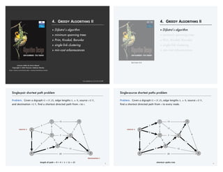
  • 1. Lecture slides by Kevin Wayne
 Copyright © 2005 Pearson-Addison Wesley
 http://www.cs.princeton.edu/~wayne/kleinberg-tardos Last updated on 2/25/20 4:16 PM 4. GREEDY ALGORITHMS II ‣ Dijkstra′s algorithm ‣ minimum spanning trees ‣ Prim, Kruskal, Boruvka ‣ single-link clustering ‣ min-cost arborescences 4. GREEDY ALGORITHMS II ‣ Dijkstra′s algorithm ‣ minimum spanning trees ‣ Prim, Kruskal, Boruvka ‣ single-link clustering ‣ min-cost arborescences SECTION 4.4 Single-pair shortest path problem Problem. Given a digraph G = (V, E), edge lengths ℓe ≥ 0, source s ∈ V, and destination t ∈ V, find a shortest directed path from s to t. 3 7 1 3 source s 6 8 5 7 5 4 15 3 12 20 13 9 destination t length of path = 9 + 4 + 1 + 11 = 25 0 4 5 2 6 9 4 1 11 Single-source shortest paths problem Problem. Given a digraph G = (V, E), edge lengths ℓe ≥ 0, source s ∈ V, find a shortest directed path from s to every node. 4 7 1 3 source s 6 8 5 7 5 4 15 3 12 20 13 9 shortest-paths tree 4 5 2 6 4 1 11 9 0
  • 2. Suppose that you change the length of every edge of G as follows.
 For which is every shortest path in G a shortest path in G′? 
 A. Add 17. B. Multiply by 17. C. Either A or B. D. Neither A nor B. 5 Shortest paths: quiz 1 s t 1 2 3 7 24 — 19 — 18 — 20 — Shortest paths: quiz 2 Which variant in car GPS? A. Single source: from one node s to every other node. B. Single sink: from every node to one node t. C. Source–sink: from one node s to another node t. D. All pairs: between all pairs of nodes. 6 Shortest path applications ・PERT/CPM. ・Map routing. ・Seam carving. ・Robot navigation. ・Texture mapping. ・Typesetting in LaTeX. ・Urban traffic planning. ・Telemarketer operator scheduling. ・Routing of telecommunications messages. ・Network routing protocols (OSPF, BGP, RIP). ・Optimal truck routing through given traffic congestion pattern. 7 Network Flows: Theory, Algorithms, and Applications, by Ahuja, Magnanti, and Orlin, Prentice Hall, 1993. Dijkstra′s algorithm (for single-source shortest paths problem) Greedy approach. Maintain a set of explored nodes S for which algorithm has determined d[u] = length of a shortest s↝u path. ・Initialize S ← { s }, d[s] ← 0. ・Repeatedly choose unexplored node v ∉ S which minimizes 8 s v u S d[u] the length of a shortest path from s to some node u in explored part S, followed by a single edge e = (u, v) (v) = min e = (u,v) : u S d[u] + e ℓe
  • 3. Greedy approach. Maintain a set of explored nodes S for which algorithm has determined d[u] = length of a shortest s↝u path. ・Initialize S ← { s }, d[s] ← 0. ・Repeatedly choose unexplored node v ∉ S which minimizes add v to S, and set d[v] ← π(v). ・To recover path, set pred[v] ← e that achieves min. Dijkstra′s algorithm (for single-source shortest paths problem) 9 s v u S d[u] d[v] (v) = min e = (u,v) : u S d[u] + e the length of a shortest path from s to some node u in explored part S, followed by a single edge e = (u, v) ℓe Invariant. For each node u ∈ S : d[u] = length of a shortest s↝u path. Pf. [ by induction on ⎜S⎟ ] Base case: ⎜S⎟ = 1 is easy since S = { s } and d[s] = 0. Inductive hypothesis: Assume true for ⎜S⎟ ≥ 1. ・Let v be next node added to S, and let (u, v) be the final edge. ・A shortest s↝u path plus (u, v) is an s↝v path of length π(v). ・Consider any other s↝v path P. We show that it is no shorter than π(v). ・Let e = (x, y) be the first edge in P that leaves S, and let Pʹ be the subpath from s to x. ・The length of P is already ≥ π (v) as soon as it reaches y: S s Dijkstra′s algorithm: proof of correctness 10 ℓ(P) ≥ ℓ(Pʹ) + ℓe non-negative lengths v u y P x Dijkstra chose v instead of y ≥ π (v) definition of π(y) ≥ π (y) inductive hypothesis ≥ d[x] + ℓe ▪ Pʹ e Dijkstra′s algorithm: efficient implementation Critical optimization 1. For each unexplored node v ∉ S : explicitly maintain π[v] instead of computing directly from definition ・For each v ∉ S : π(v) can only decrease (because set S increases). ・More specifically, suppose u is added to S and there is an edge e = (u, v) leaving u. Then, it suffices to update: Critical optimization 2. Use a min-oriented priority queue (PQ) to choose an unexplored node that minimizes π[v]. 11 π[v] ← min { π[v], π[u] + ℓe) } (v) = min e = (u,v) : u S d[u] + e recall: for each u ∈ S, π[u] = d[u] = length of shortest s↝u path Dijkstra’s algorithm: efficient implementation Implementation. ・Algorithm maintains π[v] for each node v. ・Priority queue stores unexplored nodes, using π[⋅] as priorities. ・Once u is deleted from the PQ, π[u] = length of a shortest s↝u path. 12 DIJKSTRA (V, E, ℓ, s) _________________________________________________________________________________________________________________________________________________________________________________________________________________________________________________________________________________________________________________________________________________________________________________________________________________________________________________________________________________________________________________________________________________________________________________________________________________________________________________________________________________________________________________________________________________________________________________________________________________________________________________________________________________________________________________________________________________________________________________________________________________________________________________________________________________________________________________________________________________________________________________________________________________________________________________________ FOREACH v ≠ s : π[v] ← ∞, pred[v] ← null; π[s] ← 0. Create an empty priority queue pq. FOREACH v ∈ V : INSERT(pq, v, π[v]). WHILE (IS-NOT-EMPTY(pq)) u ← DEL-MIN(pq). FOREACH edge e = (u, v) ∈ E leaving u: IF (π[v] > π[u] + ℓe) DECREASE-KEY(pq, v, π[u] + ℓe). π[v] ← π[u] + ℓe ; pred[v] ← e.
  • 4. Dijkstra′s algorithm: which priority queue? Performance. Depends on PQ: n INSERT, n DELETE-MIN, ≤ m DECREASE-KEY. ・Array implementation optimal for dense graphs. ・Binary heap much faster for sparse graphs. ・4-way heap worth the trouble in performance-critical situations. 13 priority queue INSERT DELETE-MIN DECREASE-KEY total node-indexed array (A[i] = priority of i) O(1) O(n) O(1) O(n2 ) binary heap O(log n) O(log n) O(log n) O(m log n) d-way heap
 (Johnson 1975) O(d logd n) O(d logd n) O(logd n) O(m logm/n n) Fibonacci heap
 (Fredman–Tarjan 1984) O(1) O(log n) † O(1) † O(m + n log n) integer priority queue
 (Thorup 2004) O(1) O(log log n) O(1) O(m + n log log n) † amortized Θ(n2 ) edges Θ(n) edges assumes m ≥ n How to solve the the single-source shortest paths problem in undirected graphs with positive edge lengths? 
 A. Replace each undirected edge with two antiparallel edges of same length. Run Dijkstra’s algorithm in the resulting digraph. B. Modify Dijkstra’s algorithms so that when it processes node u,
 it consider all edges incident to u (instead of edges leaving u). C. Either A or B. D. Neither A nor B. 14 Shortest paths: quiz 3 Theorem. [Thorup 1999] Can solve single-source shortest paths problem in undirected graphs with positive integer edge lengths in O(m) time. Remark. Does not explore nodes in increasing order of distance from s. 15 Shortest paths: quiz 3 Extensions of Dijkstra’s algorithm Dijkstra’s algorithm and proof extend to several related problems: ・Shortest paths in undirected graphs: π[v] ≤ π[u] + ℓ(u, v). ・Maximum capacity paths: π[v] ≥ min { π[u], c(u, v) }. ・Maximum reliability paths: π[v] ≥ π[u] 𐄂 γ(u, v) . ・… Key algebraic structure. Closed semiring (min-plus, bottleneck, Viterbi, …). 16 s v u S π[u] ℓe Fun with Semirings A functional pearl on the abuse of linear algebra Stephen Dolan Computer Laboratory, University of Cambridge stephen.dolan@cl.cam.ac.uk Abstract Describing a problem using classical linear algebra is a very well- known problem-solving technique. If your question can be formu- lated as a question about real or complex matrices, then the answer can often be found by standard techniques. It’s less well-known that very similar techniques still apply where instead of real or complex numbers we have a closed semir- ing, which is a structure with some analogue of addition and multi- plication that need not support subtraction or division. We define a typeclass in Haskell for describing closed semir- ings, and implement a few functions for manipulating matrices and polynomials over them. We then show how these functions can be used to calculate transitive closures, find shortest or longest or widest paths in a graph, analyse the data flow of imperative programs, optimally pack knapsacks, and perform discrete event simulations, all by just providing an appropriate underlying closed semiring. Categories and Subject Descriptors D.1.1 [Programming Tech- niques]: Applicative (Functional) Programming; G.2.2 [Discrete Mathematics]: Graph Theory—graph algorithms Keywords closed semirings; transitive closure; linear systems; shortest paths 1. Introduction Linear algebra provides an incredibly powerful problem-solving toolbox. A great many problems in computer graphics and vision, machine learning, signal processing and many other areas can be solved by simply expressing the problem as a system of linear equations and solving using standard techniques. Linear algebra is defined abstractly in terms of fields, of which the real and complex numbers are the most familiar examples. Fields are sets equipped with some notion of addition and multi- plication as well as negation and reciprocals. Many discrete mathematical structures commonly encountered in computer science do not have sensible notions of negation. Booleans, sets, graphs, regular expressions, imperative programs, datatypes and various other structures can all be given natural no- tions of product (interpreted variously as intersection, sequencing or conjunction) and sum (union, choice or disjunction), but gener- ally lack negation or reciprocals. Such structures, having addition and multiplication (which dis- tribute in the usual way) but not in general negation or reciprocals, are called semirings. Many structures specifying sequential actions can be thought of as semirings, with multiplication as sequencing and addition as choice. The distributive law then states, intuitively, a followed by a choice between b and c is the same as a choice between a followed by b and a followed by c. Plain semirings are a very weak structure. We can find many examples of them in the wild, but unlike fields which provide the toolbox of linear algebra, there isn’t much we can do with something knowing only that it is a semiring. However, we can build some useful tools by introducing the closed semiring, which is a semiring equipped with an extra opera- tion called closure. With the intuition of multiplication as sequenc- ing and addition as choice, closure can be interpreted as iteration. As we see in the following sections, it is possible to use something akin to Gaussian elimination on an arbitrary closed semiring, giv- ing us a means of solving certain “linear” equations over any struc- ture with suitable notions of sequencing, choice and iteration. First, though, we need to define the notion of semiring more precisely. 2. Semirings We define a semiring formally as consisting of a set R, two distin- guished elements of R named 0 and 1, and two binary operations + and ·, satisfying the following relations for any a, b, c 2 R: a + b = b + a a + (b + c) = (a + b) + c a + 0 = a a · (b · c) = (a · b) · c a · 0 = 0 · a = 0 a · 1 = 1 · a = a a · (b + c) = a · b + a · c (a + b) · c = a · c + b · c We often write a · b as ab, and a · a · a as a3 . Our focus will be on closed semirings [12], which are semir- ings with an additional operation called closure (denoted ⇤ ) which satisfies the axiom: a⇤ = 1 + a · a⇤ = 1 + a⇤ · a If we have an affine map x 7! ax + b in some closed semiring, then x = a⇤ b is a fixpoint, since a⇤ b = (aa⇤ + 1)b = a(a⇤ b) + b. So, a closed semiring can also be thought of as a semiring where affine maps have fixpoints. Fun with Semirings A functional pearl on the abuse of linear algebra Stephen Dolan Computer Laboratory, University of Cambridge stephen.dolan@cl.cam.ac.uk Abstract Describing a problem using classical linear algebra is a very well- known problem-solving technique. If your question can be formu- lated as a question about real or complex matrices, then the answer can often be found by standard techniques. It’s less well-known that very similar techniques still apply where instead of real or complex numbers we have a closed semir- ing, which is a structure with some analogue of addition and multi- plication that need not support subtraction or division. We define a typeclass in Haskell for describing closed semir- ings, and implement a few functions for manipulating matrices and polynomials over them. We then show how these functions can be used to calculate transitive closures, find shortest or longest or widest paths in a graph, analyse the data flow of imperative programs, optimally pack knapsacks, and perform discrete event simulations, all by just providing an appropriate underlying closed semiring. Categories and Subject Descriptors D.1.1 [Programming Tech- niques]: Applicative (Functional) Programming; G.2.2 [Discrete Mathematics]: Graph Theory—graph algorithms Keywords closed semirings; transitive closure; linear systems; shortest paths 1. Introduction Linear algebra provides an incredibly powerful problem-solving toolbox. A great many problems in computer graphics and vision, machine learning, signal processing and many other areas can be solved by simply expressing the problem as a system of linear equations and solving using standard techniques. Linear algebra is defined abstractly in terms of fields, of which the real and complex numbers are the most familiar examples. Fields are sets equipped with some notion of addition and multi- plication as well as negation and reciprocals. Many discrete mathematical structures commonly encountered in computer science do not have sensible notions of negation. Booleans, sets, graphs, regular expressions, imperative programs, datatypes and various other structures can all be given natural no- tions of product (interpreted variously as intersection, sequencing [Copyright notice will appear here once ’preprint’ option is removed.] or conjunction) and sum (union, choice or disjunction), but gener- ally lack negation or reciprocals. Such structures, having addition and multiplication (which dis- tribute in the usual way) but not in general negation or reciprocals, are called semirings. Many structures specifying sequential actions can be thought of as semirings, with multiplication as sequencing and addition as choice. The distributive law then states, intuitively, a followed by a choice between b and c is the same as a choice between a followed by b and a followed by c. Plain semirings are a very weak structure. We can find many examples of them in the wild, but unlike fields which provide the toolbox of linear algebra, there isn’t much we can do with something knowing only that it is a semiring. However, we can build some useful tools by introducing the closed semiring, which is a semiring equipped with an extra opera- tion called closure. With the intuition of multiplication as sequenc- ing and addition as choice, closure can be interpreted as iteration. As we see in the following sections, it is possible to use something akin to Gaussian elimination on an arbitrary closed semiring, giv- ing us a means of solving certain “linear” equations over any struc- ture with suitable notions of sequencing, choice and iteration. First, though, we need to define the notion of semiring more precisely. 2. Semirings We define a semiring formally as consisting of a set R, two distin- guished elements of R named 0 and 1, and two binary operations + and ·, satisfying the following relations for any a, b, c 2 R: a + b = b + a a + (b + c) = (a + b) + c a + 0 = a a · (b · c) = (a · b) · c a · 0 = 0 · a = 0 a · 1 = 1 · a = a a · (b + c) = a · b + a · c (a + b) · c = a · c + b · c We often write a · b as ab, and a · a · a as a3 . Our focus will be on closed semirings [12], which are semir- ings with an additional operation called closure (denoted ⇤ ) which satisfies the axiom: a⇤ = 1 + a · a⇤ = 1 + a⇤ · a If we have an affine map x 7! ax + b in some closed semiring, then x = a⇤ b is a fixpoint, since a⇤ b = (aa⇤ + 1)b = a(a⇤ b) + b. So, a closed semiring can also be thought of as a semiring where affine maps have fixpoints. The definition of a semiring translates neatly to Haskell: 1 2013/7/17
  • 5. 17 GOOGLE’S FOO.BAR CHALLENGE You have maps of parts of the space station, each starting at a prison exit and ending at the door to an escape pod. The map is represented as a matrix of 0s and 1s, where 0s are passable space and 1s are impassable walls. The door out of the prison is at the top left (0, 0) and the door into an escape pod is at the bottom right (w−1, h−1). Write a function that generates the length of a shortest path from the prison door to the escape pod, where you are allowed to remove one wall as part of your remodeling plans. s t Edsger Dijkstra 19 “ What’s the shortest way to travel from Rotterdam to Groningen? It is the algorithm for the shortest path, which I designed in about 20 minutes. One morning I was shopping in Amsterdam with my young fiancée, and tired, we sat down on the café terrace to drink a cup of coffee and I was just thinking about whether I could do this, and I then designed the algorithm for the shortest path. ” — Edsger Dijsktra The moral implications of implementing shortest-path algorithms 20 https://www.facebook.com/pg/npcompleteteens 4. GREEDY ALGORITHMS II ‣ Dijkstra′s algorithm ‣ minimum spanning trees ‣ Prim, Kruskal, Boruvka ‣ single-link clustering ‣ min-cost arborescences SECTION 6.1
  • 6. Def. A path is a sequence of edges which connects a sequence of nodes. Def. A cycle is a path with no repeated nodes or edges other than the starting and ending nodes. Cycles 22 1 2 3 4 8 5 6 7 cycle C = { (1, 2), (2, 3), (3, 4), (4, 5), (5, 6), (6, 1) } 1 6 2 3 4 5 path P = { (1, 2), (2, 3), (3, 4), (4, 5), (5, 6) } 4 8 5 Cuts Def. A cut is a partition of the nodes into two nonempty subsets S and V – S. Def. The cutset of a cut S is the set of edges with exactly one endpoint in S. 23 1 2 3 4 8 5 6 7 cutset D = { (3, 4), (3, 5), (5, 6), (5, 7), (8, 7) } 1 2 3 6 7 cut S = { 4, 5, 8 } Minimum spanning trees: quiz 1 Consider the cut S = { 1, 4, 6, 7 }. Which edge is in the cutset of S? A. S is not a cut (not connected) B. 1–7 C. 5–7 D. 2–3 24 5 4 7 1 3 8 2 6 Minimum spanning trees: quiz 2 Let C be a cycle and let D be a cutset. How many edges do C and D have in common? Choose the best answer. A. 0 B. 2 C. not 1 D. an even number 25
  • 7. Cycle–cut intersection Proposition. A cycle and a cutset intersect in an even number of edges. 26 1 2 3 4 8 5 6 7 cutset D = { (3, 4), (3, 5), (5, 6), (5, 7), (8, 7) } intersection C ∩ D = { (3, 4), (5, 6) } cycle C = { (1, 2), (2, 3), (3, 4), (4, 5), (5, 6), (6, 1) } Cycle–cut intersection Proposition. A cycle and a cutset intersect in an even number of edges. Pf. [by picture] 27 cycle C S Def. Let H = (V, T) be a subgraph of an undirected graph G = (V, E). H is a spanning tree of G if H is both acyclic and connected. Spanning tree definition 28 graph G = (V, E) spanning tree H = (V, T) Minimum spanning trees: quiz 3 Which of the following properties are true for all spanning trees H? A. Contains exactly ⎜V⎟ – 1 edges. B. The removal of any edge disconnects it. C. The addition of any edge creates a cycle. D. All of the above. 29 graph G = (V, E) spanning tree H = (V, T)
  • 8. Spanning tree properties Proposition. Let H = (V, T) be a subgraph of an undirected graph G = (V, E). Then, the following are equivalent: ・H is a spanning tree of G. ・H is acyclic and connected. ・H is connected and has ⎜V⎟ – 1 edges. ・H is acyclic and has ⎜V⎟ – 1 edges. ・H is minimally connected: removal of any edge disconnects it. ・H is maximally acyclic: addition of any edge creates a cycle. 30 graph G = (V, E) spanning tree H = (V, T) 31 https://maps.roadtrippers.com/places/46955/photos/374771356 A tree containing a cycle Minimum spanning tree (MST) Def. Given a connected, undirected graph G = (V, E) with edge costs ce, a minimum spanning tree (V, T) is a spanning tree of G such that the sum of the edge costs in T is minimized. Cayley’s theorem. The complete graph on n nodes has nn–2 spanning trees. 32 can’t solve by brute force MST cost = 50 = 4 + 6 + 8 + 5 + 11 + 9 + 7 16 4 6 23 10 21 14 24 18 9 7 11 5 8 Suppose that you change the cost of every edge in G as follows.
 For which is every MST in G an MST in G′ (and vice versa)?
 Assume c(e) > 0 for each e.
 A. cʹ(e) = c(e) + 17. B. cʹ(e) = 17 𐄂 c(e). C. cʹ(e) = log17 c(e). D. All of the above. 33 Minimum spanning trees: quiz 4
  • 9. Applications MST is fundamental problem with diverse applications. ・Dithering. ・Cluster analysis. ・Max bottleneck paths. ・Real-time face verification. ・LDPC codes for error correction. ・Image registration with Renyi entropy. ・Find road networks in satellite and aerial imagery. ・Model locality of particle interactions in turbulent fluid flows. ・Reducing data storage in sequencing amino acids in a protein. ・Autoconfig protocol for Ethernet bridging to avoid cycles in a network. ・Approximation algorithms for NP-hard problems (e.g., TSP, Steiner tree). ・Network design (communication, electrical, hydraulic, computer, road). 34 Network Flows: Theory, Algorithms, and Applications, by Ahuja, Magnanti, and Orlin, Prentice Hall, 1993. Fundamental cycle. Let H = (V, T) be a spanning tree of G = (V, E). ・For any non tree-edge e ∈ E : T ∪ { e } contains a unique cycle, say C. ・For any edge f ∈ C : (V, T ∪ { e } – { f }) is a spanning tree. Observation. If ce < cf, then (V, T) is not an MST. Fundamental cycle 35 e f graph G = (V, E) spanning tree H = (V, T) Fundamental cutset Fundamental cutset. Let H = (V, T) be a spanning tree of G = (V, E). ・For any tree edge f ∈ T : (V, T – { f }) has two connected components. ・Let D denote corresponding cutset. ・For any edge e ∈ D : (V, T – { f } ∪ { e }) is a spanning tree. Observation. If ce < cf, then (V, T) is not an MST. 36 e f graph G = (V, E) spanning tree H = (V, T) The greedy algorithm Red rule. ・Let C be a cycle with no red edges. ・Select an uncolored edge of C of max cost and color it red. Blue rule. ・Let D be a cutset with no blue edges. ・Select an uncolored edge in D of min cost and color it blue. Greedy algorithm. ・Apply the red and blue rules (nondeterministically!) until all edges are colored. The blue edges form an MST. ・Note: can stop once n – 1 edges colored blue. 37
  • 10. Greedy algorithm: proof of correctness Color invariant. There exists an MST (V, T*) containing every blue edge and no red edge. Pf. [ by induction on number of iterations ] Base case. No edges colored ⇒ every MST satisfies invariant. 38 Greedy algorithm: proof of correctness Color invariant. There exists an MST (V, T*) containing every blue edge and no red edge. Pf. [ by induction on number of iterations ] Induction step (blue rule). Suppose color invariant true before blue rule. ・let D be chosen cutset, and let f be edge colored blue. ・if f ∈ T*, then T* still satisfies invariant. ・Otherwise, consider fundamental cycle C by adding f to T*. ・let e ∈ C be another edge in D. ・e is uncolored and ce ≥ cf since - e ∈ T* ⇒ e not red - blue rule ⇒ e not blue and ce ≥ cf ・Thus, T* ∪ { f } – { e } satisfies invariant. 39 f T* e cut Greedy algorithm: proof of correctness Color invariant. There exists an MST (V, T*) containing every blue edge and no red edge. Pf. [ by induction on number of iterations ] Induction step (red rule). Suppose color invariant true before red rule. ・let C be chosen cycle, and let e be edge colored red. ・if e ∉ T*, then T* still satisfies invariant. ・Otherwise, consider fundamental cutset D by deleting e from T*. ・let f ∈ D be another edge in C. ・f is uncolored and ce ≥ cf since - f ∉ T* ⇒ f not blue - red rule ⇒ f not red and ce ≥ cf ・Thus, T* ∪ { f } – { e } satisfies invariant. ▪ 40 f T* e cut Greedy algorithm: proof of correctness Theorem. The greedy algorithm terminates. Blue edges form an MST. Pf. We need to show that either the red or blue rule (or both) applies. ・Suppose edge e is left uncolored. ・Blue edges form a forest. ・Case 1: both endpoints of e are in same blue tree. ⇒ apply red rule to cycle formed by adding e to blue forest. 41 Case 1 e
  • 11. Greedy algorithm: proof of correctness Theorem. The greedy algorithm terminates. Blue edges form an MST. Pf. We need to show that either the red or blue rule (or both) applies. ・Suppose edge e is left uncolored. ・Blue edges form a forest. ・Case 1: both endpoints of e are in same blue tree. ⇒ apply red rule to cycle formed by adding e to blue forest. ・Case 2: both endpoints of e are in different blue trees. ⇒ apply blue rule to cutset induced by either of two blue trees. ▪ 42 Case 2 e 4. GREEDY ALGORITHMS II ‣ Dijkstra′s algorithm ‣ minimum spanning trees ‣ Prim, Kruskal, Boruvka ‣ single-link clustering ‣ min-cost arborescences SECTION 6.2 Prim′s algorithm Initialize S = { s } for any node s, T = ∅. Repeat n – 1 times: ・Add to T a min-cost edge with exactly one endpoint in S. ・Add the other endpoint to S. Theorem. Prim’s algorithm computes an MST. Pf. Special case of greedy algorithm (blue rule repeatedly applied to S). ▪ 44 S by construction, edges in cutset are uncolored Prim′s algorithm: implementation Theorem. Prim’s algorithm can be implemented to run in O(m log n) time. Pf. Implementation almost identical to Dijkstra’s algorithm. 45 PRIM (V, E, c) _________________________________________________________________________________________________________________________________________________________________________________________________________________________________________________________________________________________________________________________________________________________________________________________________________________________________________________________________________________________________________________________________________________________________________________________________________________________________________________________________________________________________________________________________________________________________________________________________________________________________________________________________________________________________________________________________________________________________________________________________________________________________________________________________________________________________________________________________________________________________________________________________________________________________________________________ S ← ∅, T ← ∅. s ← any node in V. FOREACH v ≠ s : π[v] ← ∞, pred[v] ← null; π[s] ← 0. Create an empty priority queue pq. FOREACH v ∈ V : INSERT(pq, v, π[v]). WHILE (IS-NOT-EMPTY(pq)) u ← DEL-MIN(pq). S ← S ∪ { u }, T ← T ∪ { pred[u] }. FOREACH edge e = (u, v) ∈ E with v ∉ S : IF (ce < π[v]) DECREASE-KEY(pq, v, ce). π[v] ← ce; pred[v] ← e. π[v] = cost of cheapest known edge between v and S
  • 12. Kruskal′s algorithm Consider edges in ascending order of cost: ・Add to tree unless it would create a cycle. Theorem. Kruskal’s algorithm computes an MST. Pf. Special case of greedy algorithm. ・Case 1: both endpoints of e in same blue tree. ⇒ color e red by applying red rule to unique cycle. ・Case 2: both endpoints of e in different blue trees. ⇒ color e blue by applying blue rule to cutset defined by either tree. ▪ 46 e all other edges in cycle are blue no edge in cutset has smaller cost (since Kruskal chose it first) Kruskal′s algorithm: implementation Theorem. Kruskal’s algorithm can be implemented to run in O(m log m) time. ・Sort edges by cost. ・Use union–find data structure to dynamically maintain connected components. 47 KRUSKAL (V, E, c) ________________________________________________________________________________________________________________________________________________________________________________________________________________________________________________________________________________________________________________________________________________________________________________________________________________________________________________________________________________________________________________________________________________________________________________________________________________________________________________________________________________________________________________________________________________________________________________________________________________________________________________________________________________________________________________________________________________________________________________________________________________________________________________________________________________________________________________________________________________________________________________________________________________________________ SORT m edges by cost and renumber so that c(e1) ≤ c(e2) ≤ … ≤ c(em). T ← ∅. FOREACH v ∈ V : MAKE-SET(v). FOR i = 1 TO m (u, v) ← ei. IF (FIND-SET(u) ≠ FIND-SET(v)) T ← T ∪ { ei }. UNION(u, v). RETURN T. are u and v in same component? make u and v in same component Reverse-delete algorithm Start with all edges in T and consider them in descending order of cost: ・Delete edge from T unless it would disconnect T. Theorem. The reverse-delete algorithm computes an MST. Pf. Special case of greedy algorithm. ・Case 1. [ deleting edge e does not disconnect T ] ⇒ apply red rule to cycle C formed by adding e to another path in T between its two endpoints ・Case 2. [ deleting edge e disconnects T ] ⇒ apply blue rule to cutset D induced by either component ▪ 
 Fact. [Thorup 2000] Can be implemented to run in O(m log n (log log n)3) time. 48 no edge in C is more expensive (it would have already been considered and deleted) e is the only remaining edge in the cutset (all other edges in D must have been colored red / deleted) Review: the greedy MST algorithm Red rule. ・Let C be a cycle with no red edges. ・Select an uncolored edge of C of max cost and color it red. Blue rule. ・Let D be a cutset with no blue edges. ・Select an uncolored edge in D of min cost and color it blue. Greedy algorithm. ・Apply the red and blue rules (nondeterministically!) until all edges are colored. The blue edges form an MST. ・Note: can stop once n – 1 edges colored blue. Theorem. The greedy algorithm is correct. Special cases. Prim, Kruskal, reverse-delete, … 49
  • 13. Borůvka′s algorithm Repeat until only one tree. ・Apply blue rule to cutset corresponding to each blue tree. ・Color all selected edges blue. Theorem. Borůvka’s algorithm computes the MST. Pf. Special case of greedy algorithm (repeatedly apply blue rule). ▪ 50 7 11 5 8 12 13 assume edge costs are distinct Borůvka′s algorithm: implementation Theorem. Borůvka’s algorithm can be implemented to run in O(m log n) time. Pf. ・To implement a phase in O(m) time: - compute connected components of blue edges - for each edge (u, v) ∈ E, check if u and v are in different components; if so, update each component’s best edge in cutset ・≤ log2 n phases since each phase (at least) halves total # components. ▪ 51 7 11 5 8 12 13 Borůvka′s algorithm: implementation Contraction version. ・After each phase, contract each blue tree to a single supernode. ・Delete self-loops and parallel edges (keeping only cheapest one). ・Borůvka phase becomes: take cheapest edge incident to each node. Q. How to contract a set of edges? 52 2 3 5 4 6 1 8 3 4 2 9 7 5 6 3 4 6 1 8 3 2 9 7 5 6 2, 5 3 4 6 1 8 3 2 9 7 5 2, 5 graph G contract edge 2-5 delete self-loops and parallel edges 1 1 1 Problem. Given a graph G = (V, E) and a set of edges F, contract all edges in F, removing any self-loops or parallel edges. Goal. O(m + n) time. CONTRACT A SET OF EDGES 53 graph G contracted graph G′
  • 14. CONTRACT A SET OF EDGES Problem. Given a graph G = (V, E) and a set of edges F, contract all edges in F, removing any self-loops or parallel edges. Solution. ・Compute the nʹ connected components in (V, F). ・Suppose id[u] = i means node u is in connected component i. ・The contracted graph Gʹ has nʹ nodes. ・For each edge u–v ∈ E, add an edge i–j to Gʹ, where i = id[u] and j = id[v]. Removing self loops. Easy. Removing parallel edges. ・Create a list of edges i–j with the convention that i < j. ・Sort the edges lexicographically via LSD radix sort. ・Add the edges to the graph Gʹ, removing parallel edges. 54 Theorem. Borůvka’s algorithm (contraction version) can be implemented to run in O(n) time on planar graphs. Pf. ・Each Borůvka phase takes O(n) time: - Fact 1: m ≤ 3n for simple planar graphs. - Fact 2: planar graphs remains planar after edge contractions/deletions. ・Number of nodes (at least) halves in each phase. ・Thus, overall running time ≤ cn + cn / 2 + cn / 4 + cn / 8 + … = O(n). ▪ Borůvka′s algorithm on planar graphs 55 planar K3,3 not planar A hybrid algorithm Borůvka–Prim algorithm. ・Run Borůvka (contraction version) for log2 log2 n phases. ・Run Prim on resulting, contracted graph. Theorem. Borůvka–Prim computes an MST. Pf. Special case of the greedy algorithm. Theorem. Borůvka–Prim can be implemented to run in O(m log log n) time. Pf. ・The log2 log2 n phases of Borůvka’s algorithm take O(m log log n) time; resulting graph has ≤ n / log2 n nodes and ≤ m edges. ・Prim’s algorithm (using Fibonacci heaps) takes O(m + n) time on a graph with n / log2 n nodes and m edges. ▪ 56 O m + n log n log n log n Does a linear-time compare-based MST algorithm exist? Theorem. [Fredman–Willard 1990] O(m) in word RAM model. Theorem. [Dixon–Rauch–Tarjan 1992] O(m) MST verification algorithm. Theorem. [Karger–Klein–Tarjan 1995] O(m) randomized MST algorithm. 57 deterministic compare-based MST algorithms year worst case discovered by 1975 O(m log log n) Yao 1976 O(m log log n) Cheriton–Tarjan 1984 O(m log*n), O(m + n log n) Fredman–Tarjan 1986 O(m log (log* n)) Gabow–Galil–Spencer–Tarjan 1997 O(m α(n) log α(n)) Chazelle 2000 O(m α(n)) Chazelle 2002 asymptotically optimal Pettie–Ramachandran 20xx O(m) n lg* n (−∞, 1] 0 (1, 2] 1 (2, 4] 2 (4, 16] 3 (16, 216] 4 (216, 265536] 5 lg n = 0 n 1 1 + lg (lg n) n > 1 <latexit sha1_base64="HJFYyV8ahuzHjW6Ka99U33ko4ac=">AAACkXicbVFdaxNBFJ1s/ajrV1p98+ViUKpC2BWhraAEfRF8qWBsIRPD7OzdZOjs7DJztyQs+Yu++z/6WnGy2QeTeGGGw7nnfsyZpNTKURT97gR7t27fubt/L7z/4OGjx92Dwx+uqKzEoSx0YS8S4VArg0NSpPGitCjyRON5cvl5lT+/QutUYb7TosRxLqZGZUoK8tSkO+N6+vM1GPgQ8gSnytTSd3PLMIKXwAnnBDWoDJZewjVCDJyHMbyBpu7I32Be7Uo/roUcTdo2nHR7UT9qAnZB3IIea+NsctA55GkhqxwNSS2cG8VRSeNaWFJS4zLklcNSyEsxxZGHRuToxnVjyRJeeCaFrLD+GIKG/beiFrlzizzxylzQzG3nVuT/cqOKspNxrUxZERq5HpRVGqiAlb+QKouS9MIDIa3yu4KcCSsk+V/YmNL0LlFuvKSeV0bJIsUtVtOcrFi5GG97tguGb/un/ejbu97gpLVznz1jz9kRi9kxG7Av7IwNmWS/2DW7YX+Cp8H7YBB8WkuDTlvzhG1E8PUvXjrGCA==</latexit> <latexit sha1_base64="HJFYyV8ahuzHjW6Ka99U33ko4ac=">AAACkXicbVFdaxNBFJ1s/ajrV1p98+ViUKpC2BWhraAEfRF8qWBsIRPD7OzdZOjs7DJztyQs+Yu++z/6WnGy2QeTeGGGw7nnfsyZpNTKURT97gR7t27fubt/L7z/4OGjx92Dwx+uqKzEoSx0YS8S4VArg0NSpPGitCjyRON5cvl5lT+/QutUYb7TosRxLqZGZUoK8tSkO+N6+vM1GPgQ8gSnytTSd3PLMIKXwAnnBDWoDJZewjVCDJyHMbyBpu7I32Be7Uo/roUcTdo2nHR7UT9qAnZB3IIea+NsctA55GkhqxwNSS2cG8VRSeNaWFJS4zLklcNSyEsxxZGHRuToxnVjyRJeeCaFrLD+GIKG/beiFrlzizzxylzQzG3nVuT/cqOKspNxrUxZERq5HpRVGqiAlb+QKouS9MIDIa3yu4KcCSsk+V/YmNL0LlFuvKSeV0bJIsUtVtOcrFi5GG97tguGb/un/ejbu97gpLVznz1jz9kRi9kxG7Av7IwNmWS/2DW7YX+Cp8H7YBB8WkuDTlvzhG1E8PUvXjrGCA==</latexit> <latexit sha1_base64="HJFYyV8ahuzHjW6Ka99U33ko4ac=">AAACkXicbVFdaxNBFJ1s/ajrV1p98+ViUKpC2BWhraAEfRF8qWBsIRPD7OzdZOjs7DJztyQs+Yu++z/6WnGy2QeTeGGGw7nnfsyZpNTKURT97gR7t27fubt/L7z/4OGjx92Dwx+uqKzEoSx0YS8S4VArg0NSpPGitCjyRON5cvl5lT+/QutUYb7TosRxLqZGZUoK8tSkO+N6+vM1GPgQ8gSnytTSd3PLMIKXwAnnBDWoDJZewjVCDJyHMbyBpu7I32Be7Uo/roUcTdo2nHR7UT9qAnZB3IIea+NsctA55GkhqxwNSS2cG8VRSeNaWFJS4zLklcNSyEsxxZGHRuToxnVjyRJeeCaFrLD+GIKG/beiFrlzizzxylzQzG3nVuT/cqOKspNxrUxZERq5HpRVGqiAlb+QKouS9MIDIa3yu4KcCSsk+V/YmNL0LlFuvKSeV0bJIsUtVtOcrFi5GG97tguGb/un/ejbu97gpLVznz1jz9kRi9kxG7Av7IwNmWS/2DW7YX+Cp8H7YBB8WkuDTlvzhG1E8PUvXjrGCA==</latexit> iterated logarithm function
  • 15. MINIMUM BOTTLENECK SPANNING TREE Problem. Given a connected graph G with positive edge costs, find a spanning tree that minimizes the most expensive edge. Goal. O(m log m) time or better. 58 minimum bottleneck spanning tree T (bottleneck = 9) 6 5 9 7 8 7 14 21 3 24 4 10 11 Note: not necessarily a MST 9 4. GREEDY ALGORITHMS II ‣ Dijkstra′s algorithm ‣ minimum spanning trees ‣ Prim, Kruskal, Boruvka ‣ single-link clustering ‣ min-cost arborescences SECTION 4.7 Goal. Given a set U of n objects labeled p1, …, pn, partition into clusters so that objects in different clusters are far apart. Applications. ・Routing in mobile ad-hoc networks. ・Document categorization for web search. ・Similarity searching in medical image databases ・Cluster celestial objects into stars, quasars, galaxies. ・... Clustering outbreak of cholera deaths in London in 1850s (Nina Mishra) 62 4-clustering k-clustering. Divide objects into k non-empty groups. Distance function. Numeric value specifying “closeness” of two objects. ・d(pi, pj) = 0 iff pi = pj [ identity of indiscernibles ] ・d(pi, pj) ≥ 0 [ non-negativity ] ・d(pi, pj) = d(pj, pi) [ symmetry ] Spacing. Min distance between any pair of points in different clusters. Goal. Given an integer k, find a k-clustering of maximum spacing. Clustering of maximum spacing 63 distance between two clusters min distance between two closest clusters
  • 16. Greedy clustering algorithm “Well-known” algorithm in science literature for single-linkage k-clustering: ・Form a graph on the node set U, corresponding to n clusters. ・Find the closest pair of objects such that each object is in a different cluster, and add an edge between them. ・Repeat n – k times (until there are exactly k clusters). Key observation. This procedure is precisely Kruskal’s algorithm (except we stop when there are k connected components). Alternative. Find an MST and delete the k – 1 longest edges. 64 Greedy clustering algorithm: analysis Theorem. Let C* denote the clustering C* 1, …, C* k formed by deleting the k – 1 longest edges of an MST. Then, C* is a k-clustering of max spacing. Pf. ・Let C denote any other clustering C1, …, Ck. ・Let pi and pj be in the same cluster in C*, say C* r , but different clusters in C, say Cs and Ct. ・Some edge (p, q) on pi – pj path in C* r spans two different clusters in C. ・Spacing of C* = length d* of the (k – 1)st longest edge in MST. ・Edge (p, q) has length ≤ d* since it was added by Kruskal. ・Spacing of C is ≤ d* since p and q are in different clusters. ▪ 65 p q pi pj Cs Ct C* r edges left after deleting k – 1 longest edges from a MST this is the edge Kruskal would have added next had we not stopped it Dendrogram of cancers in human Tumors in similar tissues cluster together. Reference: Botstein & Brown group gene 1 gene n gene expressed gene not expressed 66 Which MST algorithm should you use for single-link clustering?
 A. Kruskal (stop when there are k components). B. Prim (delete k – 1 longest edges). C. Either A or B. D. Neither A nor B. 67 Minimum spanning trees: quiz 5 number of objects n can be very large
  • 17. 4. GREEDY ALGORITHMS II ‣ Dijkstra′s algorithm ‣ minimum spanning trees ‣ Prim, Kruskal, Boruvka ‣ single-link clustering ‣ min-cost arborescences SECTION 4.9 Arborescences Def. Given a digraph G = (V, E) and a root r ∈ V, an arborescence (rooted at r) is a subgraph T = (V, F) such that ・T is a spanning tree of G if we ignore the direction of edges. ・There is a (unique) directed path in T from r to each other node v ∈ V. 69 r Which of the following are properties of arborescences rooted at r?
 A. No directed cycles. B. Exactly n − 1 edges. C. For each v ≠ r : indegree(v) = 1. D. All of the above. 70 Minimum spanning arborescence: quiz 1 r Arborescences Proposition. A subgraph T = (V, F) of G is an arborescence rooted at r iff T has no directed cycles and each node v ≠ r has exactly one entering edge. Pf. ⇒ If T is an arborescence, then no (directed) cycles and every node v ≠ r has exactly one entering edge—the last edge on the unique r↝v path. ⇐ Suppose T has no cycles and each node v ≠ r has one entering edge. ・To construct an r↝v path, start at v and repeatedly follow edges in the backward direction. ・Since T has no directed cycles, the process must terminate. ・It must terminate at r since r is the only node with no entering edge. ▪
 71
  • 18. Given a digraph G, how to find an arborescence rooted at r?
 A. Breadth-first search from r. B. Depth-first search from r. C. Either A or B. D. Neither A nor B. 72 Minimum spanning arborescence: quiz 2 r Min-cost arborescence problem Problem. Given a digraph G with a root node r and edge costs ce ≥ 0, find an arborescence rooted at r of minimum cost. Assumption 1. All nodes reachable from r. Assumption 2. No edge enters r (safe to delete since they won’t help). 73 r 4 1 2 3 5 6 9 7 8 A min-cost arborescence must…
 A. Include the cheapest edge. B. Exclude the most expensive edge. C. Be a shortest-paths tree from r. D. None of the above. 74 Minimum spanning arborescence: quiz 3 r 8 3 4 6 10 12 A sufficient optimality condition Property. For each node v ≠ r, choose a cheapest edge entering v and let F* denote this set of n – 1 edges. If (V, F*) is an arborescence, then it is a min-cost arborescence. Pf. An arborescence needs exactly one edge entering each node v ≠ r and (V, F*) is the cheapest way to make each of these choices. ▪ 75 r 4 2 1 3 5 6 9 7 8 F* = thick black edges
  • 19. A sufficient optimality condition Property. For each node v ≠ r, choose a cheapest edge entering v and let F* denote this set of n – 1 edges. If (V, F*) is an arborescence, then it is a min-cost arborescence. Note. F* may not be an arborescence (since it may have directed cycles). 76 r 4 1 2 3 5 6 9 7 8 F* = thick black edges Reduced costs Def. For each v ≠ r, let y(v) denote the min cost of any edge entering v. Define the reduced cost of an edge (u, v) as cʹ(u, v) = c(u, v) – y(v) ≥ 0. Observation. T is a min-cost arborescence in G using costs c iff T is a min-cost arborescence in G using reduced costs cʹ. Pf. For each v ≠ r : each arborescence has exactly one edge entering v. ▪ 77 r 4 1 2 3 7 9 r 0 0 1 0 3 0 costs c reduced costs c′ 1 9 4 3 y(v) Intuition. Recall F* = set of cheapest edges entering v for each v ≠ r. ・Now, all edges in F* have 0 cost with respect to reduced costs cʹ(u, v). ・If F* does not contain a cycle, then it is a min-cost arborescence. ・If F* contains a cycle C, can afford to use as many edges in C as desired. ・Contract edges in C to a supernode (removing any self-loops). ・Recursively solve problem in contracted network Gʹ with costs cʹ(u, v). Edmonds branching algorithm: intuition 78 r 0 3 4 1 0 0 0 4 0 0 7 1 0 F* = thick edges Edmonds branching algorithm: intuition Intuition. Recall F* = set of cheapest edges entering v for each v ≠ r. ・Now, all edges in F* have 0 cost with respect to reduced costs cʹ(u, v). ・If F* does not contain a cycle, then it is a min-cost arborescence. ・If F* contains a cycle C, can afford to use as many edges in C as desired. ・Contract edges in C to a supernode (removing any self-loops). ・Recursively solve problem in contracted network Gʹ with costs cʹ(u, v). 79 r 3 4 0 0 7 1 1 0
  • 20. Edmonds branching algorithm 80 EDMONDS-BRANCHING (G, r , c) _________________________________________________________________________________________________________________________________________________________________________________________________________________________________________________________________________________________________________________________________________________________________________________________________________________________________________________________________________________________________________________________________________________________________________________________________________________________________________________________________________________________________________________________________________________________________________________________________________________________________________________________________________________________________________________________________________________________________________________________________________________________________________________________________________________________________________________________________________________________________________________________________________________________________________________________________________________________________________________________________________________________________________________________________________________________________________________ FOREACH v ≠ r : y(v) ← min cost of any edge entering v. cʹ(u, v) ← cʹ(u, v) – y(v) for each edge (u, v) entering v. FOREACH v ≠ r : choose one 0-cost edge entering v and let F* be the resulting set of edges. IF (F* forms an arborescence) RETURN T = (V, F*). ELSE C ← directed cycle in F*. Contract C to a single supernode, yielding Gʹ = (Vʹ, Eʹ). T ʹ ← EDMONDS-BRANCHING(Gʹ, r , cʹ). Extend T ʹ to an arborescence T in G by adding all but one edge of C. RETURN T. _________________________________________________________________________________________________________________________________________________________________________________________________________________________________________________________________________________________________________________________________________________________________________________________________________________________________________________________________________________________________________________________________________________________________________________________________________________________________________________________________________________________________________________________________________________________________________________________________________________________________________________________________________________________________________________________________________________________________________________________________________________________________________________________________________________________________________________________________________________________________________________________________________________________________________________________________________________________________________________________________________________________________________________________________________________________________________________ Edmonds branching algorithm Q. What could go wrong? A. Contracting cycle C places extra constraint on arborescence. ・Min-cost arborescence in Gʹ must have exactly one edge entering a node in C (since C is contracted to a single node) ・But min-cost arborescence in G might have several edges entering C. 81 b a r cycle C min-cost arborescence in G Edmonds branching algorithm: key lemma Lemma. Let C be a cycle in G containing only 0-cost edges. There exists a min-cost arborescence T rooted at r that has exactly one edge entering C. Pf. Case 0. T has no edges entering C. Since T is an arborescence, there is an r↝v path for each node v ⇒ at least one edge enters C. ※ Case 1. T has exactly one edge entering C. T satisfies the lemma. Case 2. T has two (or more) edges entering C. We construct another min-cost arborescence T * that has exactly one edge entering C. 82 Edmonds branching algorithm: key lemma Case 2 construction of T *. ・Let (a, b) be an edge in T entering C that lies on a shortest path from r. ・We delete all edges of T that enter a node in C except (a, b). ・We add in all edges of C except the one that enters b. b 83 a r cycle C T this path from r to C uses only one node in C
  • 21. T Edmonds branching algorithm: key lemma Case 2 construction of T *. ・Let (a, b) be an edge in T entering C that lies on a shortest path from r. ・We delete all edges of T that enter a node in C except (a, b). ・We add in all edges of C except the one that enters b. Claim. T * is a min-cost arborescence. ・The cost of T * is at most that of T since we add only 0-cost edges. ・T * has exactly one edge entering each node v ≠ r. ・T * has no directed cycles. (T had no cycles before; no cycles within C; now only (a, b) enters C) b 84 b a T is an arborescence rooted at r r cycle C T* and the only path in T * to a is the path from r to a (since any path must follow unique entering edge back to r) this path from r to C uses only one node in C Edmonds branching algorithm: analysis Theorem. [Chu–Liu 1965, Edmonds 1967] The greedy algorithm finds a min-cost arborescence. Pf. [ by strong induction on number of nodes ] ・If the edges of F* form an arborescence, then min-cost arborescence. ・Otherwise, we use reduced costs, which is equivalent. ・After contracting a 0-cost cycle C to obtain a smaller graph Gʹ, the algorithm finds a min-cost arborescence T ʹ in Gʹ (by induction). ・Key lemma: there exists a min-cost arborescence T in G that corresponds to T ʹ. ▪ 
 Theorem. The greedy algorithm can be implemented to run in O(m n) time. Pf. ・At most n contractions (since each reduces the number of nodes). ・Finding and contracting the cycle C takes O(m) time. ・Transforming T ʹ into T takes O(m) time. ▪ 85 un-contracting cycle C, remove all but one edge entering C, taking all but one edge in C Min-cost arborescence Theorem. [Gabow–Galil–Spencer–Tarjan 1985] There exists an O(m + n log n) time algorithm to compute a min-cost arborescence. 86