SlideShare uma empresa Scribd logo
1 de 29
Variational AutoEncoder
Kang, Min-Guk
1
Z 𝑝 𝜃(. ) X
Decoder
X 𝑞∅(. )
Encoder
𝜇
𝜎
𝑍 = 𝜇 + 𝜎𝜀
Where 𝜀 ~ N(0,1)
Reparameterization trick
𝑞∅ 𝑍 𝑋
Variational Inference
𝑝 𝜃(𝑋|𝑍)
1. 들어가기 앞서 알고 있으면 좋은 지식
2
1. Manifold
Manifold란 두 점 사이의 거리 혹은 유사도가 근거리에서는 Euclidean metric을 따르지만 원거리에서는
그렇지 않은 공간을 의미한다.
2. Manifold Hypothesis
1. 고차원의 data 밀도는 낮지만, 이들의 집합을 포함하는 저차원의 Manifold가 있다.
2. 이 저차원의 Manifold를 벗어나는 순간 급격히 밀도는 낮아진다.
→ 우리의 고차원 데이터(Mnist의 경우 784차원)를 저차원 Manifold로 차원감소를 시키면, 데이터의 분포가
조밀해지고 데이터를 서로 비교할 수 있는 Boundary가 생긴다.
1. 들어가기 앞서 알고 있으면 좋은 지식
3
고차원의 MNIST 데이터
VAE를 이용해 차원감소를 시킨
2D- MNIST 데이터
1. 들어가기 앞서 알고 있으면 좋은 지식
4
첫 번째 사진과 세 번째 사진의 중간을 찾고 싶을 때는 유클리디안 거리를 이용하면 안된다!
자료 출처: https://www.facebook.com/groups/TensorFlowKR/permalink/496009234073473/?hc_location=ufi
다운로드: https://mega.nz/#!tBo3zAKR!yE6tZ0g-GyUyizDf7uglDk2_ahP-zj5trVZSLW3GAjw
(Hwalsuk Lee님 슬라이드 자료에서 따왔습니다.)
1. 들어가기 앞서 알고 있으면 좋은 지식
5
Manifold 공간 상 중간에 있는 값을 사용해야 좋은 예측을 할 수 있다!
자료 출처: https://www.facebook.com/groups/TensorFlowKR/permalink/496009234073473/?hc_location=ufi
다운로드: https://mega.nz/#!tBo3zAKR!yE6tZ0g-GyUyizDf7uglDk2_ahP-zj5trVZSLW3GAjw
(Hwalsuk Lee님 슬라이드 자료에서 따왔습니다.)
1. 들어가기 앞서 알고 있으면 좋은 지식
6
3. Bayes Rule
𝑃 𝑋 𝑌 =
𝑃(𝑌|𝑋)𝑃(𝑋)
𝑃(𝑌)
4. KL-Divergence
𝐷 𝐾𝐿 𝑃 𝑄 =
𝑖
𝑝 𝑖 𝑙𝑜𝑔
𝑃 𝑖
𝑄 𝑖
두 확률 분포 P, Q사이의 유사도를 측정하는 방법으로, 값이 작을 수록 두 확률분포가 유사하며,
항상 0보다 큰 특징을 가지고 있다.
likelihood
prior
Normalize term
posterior
2. Variational AutoEncoder
우리의 목표는 Normal distribution N(0,1) 에서 Z를 샘플링을 한 후 이를 이용하여 X라는 데이터를 생성하는 것이다.
즉 그림으로 표현을 하면 아래와 같다.
N(0,1) ~ Z 𝑝 𝜃(𝑋|𝑍) X
Decoder
𝑝 𝜃(𝑋|𝑍)를 Gaussian distribution으로 가정하게 되면
이 문제는 p x = 𝑝 𝑥 𝑔 𝜃 𝑧 𝑝(𝑧)𝑑𝑧를 최대화 해주는 MLE문제가 된다.
하지만,
7
2. Variational AutoEncoder
위의 논문에도 나와있듯 P(X|Z)를 Gaussian distribution으로 가정하고, -log(P(X))를 Minimize 할 시 데이터 사이의
Euclidian distance가 작아지도록 학습이 일어나 학습이 정확한 방향으로 되지 않는다.
Figure 3의 (a)라는 데이터를 이용해 학습을 했다고 하면 (c)라는 결과가 나와야 좋은데, Euclidian distance가 가까운
(b)가 생성된다.
Tutorial on Variational Autoencoders : https://arxiv.org/pdf/1606.05908 8
2. Variational AutoEncoder
이를 해결하기 위해 Z를 무작정 N(0,1)에서 샘플링 하는 것이 아닌, 내가 가지고 있는 Input data X를 이용하여
Sampling을 한 것이 Variational AutoEncoder 이다.
Z 𝑝 𝜃(. ) X
Decoder
X 𝑞 𝜃(. )
Encoder
9
2. Variational AutoEncoder
문제점
① 𝑞 𝜃(𝑍|𝑋)를 계산 할 수 없음. Intractable함.
→ 𝑞∅(𝑍|𝑋)라는 확률분포를 정의해주고 KL-Divergence를 이용해 근사 시켜준다(Variational Inference).
② Backpropagation을 하려면 모델이 미분가능 해야 하는데 𝑞∅(𝑍|𝑋)는 미분 불가능하다.
→ Reparameterization Trick을 이용해 해결, 논문의 first contribution.
Z 𝑝 𝜃(𝑋|𝑍) X
Decoder
X 𝑞 𝜃(𝑍|𝑋)
Encoder
10
2. Variational AutoEncoder
11
문제점
① 𝑞 𝜃(𝑍|𝑋)를 계산 할 수 없음. Intractable함. 아래의 cs231n slide 참조.
출처: http://cs231n.stanford.edu/
2. Variational AutoEncoder
12
문제점
① 𝑞 𝜃(𝑍|𝑋)를 계산 할 수 없음. Intractable함. 아래의 cs231n slide 참조.
→ 𝑞∅(𝑋|𝑍)라는 확률분포를 정의해주고 KL-Divergence를 이용해 근사 시켜준다(Variational Inference).
𝑞∅(𝑍|𝑋)를 Gaussian distribution으로 가정하면, 우리의 네트워크는 아래와 같이 된다.
Z 𝑝 𝜃(. ) X
Decoder
X 𝑞∅(. )
Encoder
𝜇
𝜎
N(𝜇,𝜎) ~
2. Variational AutoEncoder
13
이 부분이 문제!
문제점
② Backpropagation을 하려면 모델이 미분가능 해야 하는데 𝑞∅(𝑍|𝑋)는 미분 불가능하다.
→ Reparameterization Trick을 이용해 해결, 논문의 first contribution.
Z 𝑝 𝜃(. ) X
Decoder
X 𝑞∅(. )
Encoder
𝜇
𝜎
N(𝜇,𝜎) ~
2. Variational AutoEncoder
14
문제점
② Backpropagation을 하려면 모델이 미분가능 해야 하는데 𝑞∅(𝑋|𝑍)는 미분 불가능하다.
→ Reparameterization Trick을 이용해 해결, 논문의 first contribution.
Z 𝑝 𝜃(. ) X
Decoder
X 𝑞∅(. )
Encoder
𝜇
𝜎
𝑍 = 𝜇 + 𝜎𝜀
Where 𝜀 ~ N(0,1)
Reparameterization trick
3. 수학(Maximum Marginal loglikelihood Estimation)
15
log 𝑃 𝜃 𝑋 = 1 × log 𝑃 𝜃 𝑋
=
𝑧
𝑃 𝜃 𝑍 𝑋 × log 𝑃 𝜃 𝑋
≈
𝑧
𝑞∅ 𝑍 𝑋 × log 𝑃 𝜃 𝑋 =
𝑧
𝑞∅ 𝑍 𝑋 × log
𝑃 𝜃 𝑋, 𝑍
𝑃 𝜃 𝑍 𝑋
=
𝑧
𝑞∅ 𝑍 𝑋 × log
𝑃 𝜃 𝑋, 𝑍
𝑞∅ 𝑍 𝑋
×
𝑞∅ 𝑍 𝑋
𝑃 𝜃 𝑍 𝑋
=
𝑍
𝑞∅ 𝑍 𝑋 × log
𝑃 𝜃 𝑋, 𝑍
𝑞∅ 𝑍 𝑋
+
𝑍
𝑞∅(𝑍|𝑋) × log(
𝑞∅ 𝑍 𝑋
𝑃 𝜃 𝑍 𝑋
)
𝐾𝐿 − 𝐷𝑖𝑣𝑒𝑟𝑔𝑒𝑛𝑐𝑒의 정의에 의해 준 식은 다음과 같이 바뀐다.
=
𝑍
𝑞∅ 𝑍 𝑋 × log
𝑃 𝜃 𝑋, 𝑍
𝑞∅ 𝑍 𝑋
+ 𝐷 𝐾𝐿(𝑞∅(𝑍|𝑋)| 𝑃 𝜃 𝑍 𝑋 = 𝐿(𝑎) 𝜃, ∅; 𝑋 + 𝐷 𝐾𝐿(𝑞∅(𝑍|𝑋)| 𝑃 𝜃 𝑍 𝑋 … (1)
3. 수학(Maximum Marginal loglikelihood Estimation)
16
log 𝑃 𝜃 𝑋 =
𝑍
𝑞∅ 𝑍 𝑋 × log
𝑃 𝜃 𝑋, 𝑍
𝑞∅ 𝑍 𝑋
+ 𝐷 𝐾𝐿(𝑞∅(𝑍|𝑋)| 𝑃 𝜃 𝑍 𝑋 = 𝐿(𝑎)
𝜃, ∅; 𝑋 + 𝐷 𝐾𝐿(𝑞∅(𝑍|𝑋)| 𝑃 𝜃 𝑍 𝑋 … (1)
위의 식의 𝐿(𝑎)
𝜃, ∅; 𝑋 부분을 조금만 더 전개해보자.
𝑍
𝑞∅ 𝑍 𝑋 × log
𝑃 𝜃 𝑋, 𝑍
𝑞∅ 𝑍 𝑋
=
𝑍
𝑞∅(𝑍|𝑋) × log(
𝑃 𝜃 𝑋, 𝑍 × 𝑃 𝜃 𝑍
𝑃 𝜃 𝑍 × 𝑞∅ 𝑍 𝑋
)
=
𝑍
𝑞∅(𝑍|𝑋) × log
𝑃 𝜃 𝑋, 𝑍
𝑃 𝜃 𝑍
−
𝑍
𝑞∅(𝑍|𝑋) × log
𝑞∅ 𝑍 𝑋
𝑃 𝜃 𝑍
= 𝑍
𝑞∅(𝑍|𝑋) × log 𝑃 𝜃 𝑋|𝑍 − 𝐷 𝐾𝐿(𝑞∅(𝑍|𝑋)| 𝑃 𝜃 𝑍 = 𝐿(𝑏)
𝜃, ∅; 𝑋 − 𝐷 𝐾𝐿(𝑞∅(𝑍|𝑋)| 𝑃 𝜃 𝑍 …(2)
∴ log 𝑃 𝜃 𝑋 = 𝐿(𝑎)
𝜃, ∅; 𝑋 + 𝐷 𝐾𝐿(𝑞∅(𝑍|𝑋)| 𝑃 𝜃 𝑍 𝑋 ≥ 𝐿(𝑎)
𝜃, ∅; 𝑋 이므로 Lower bound인 𝐿(𝑎)
𝜃, ∅; 𝑋 를 최대화 하면
log 𝑃 𝜃 𝑋 값도 최대가 된다고 생각할 수 있다.
3. 수학(Maximum Marginal loglikelihood Estimation)
17
log 𝑃 𝜃 𝑋 = 𝐿(𝑎)
𝜃, ∅; 𝑋 + 𝐷 𝐾𝐿(𝑞∅(𝑍|𝑋)| 𝑃 𝜃 𝑍 𝑋 ≥ 𝐿(𝑎)
𝜃, ∅; 𝑋 이므로 Lower bound인 𝐿(𝑎)
𝜃, ∅; 𝑋 를 최대화 하면
log 𝑃 𝜃 𝑋 값도 최대가 된다고 생각할 수 있다. 따라서 우리의 목표는 다음과 같이 다시 작성될 수 있다.
𝐴𝑟𝑔𝑚𝑎𝑥 𝜃 log 𝑃 𝜃 𝑋 ↔ 𝐴𝑟𝑔𝑚𝑎𝑥 𝜃,∅(𝐿 𝑎
𝜃, ∅; 𝑋 )
𝐴𝑟𝑔𝑚𝑎𝑥 𝜃,∅ 𝐿 𝑎
𝜃, ∅; 𝑋 = 𝐴𝑟𝑔𝑚𝑎𝑥 𝜃,∅(
𝑍
𝑞∅ 𝑍 𝑋 × log 𝑃 𝜃 𝑋|𝑍 − 𝐷 𝐾𝐿(𝑞∅(𝑍|𝑋)| 𝑃 𝜃 𝑍 )
위의 식에서 (b)는 𝑞∅(𝑍|𝑋)가 Gaussian distribution, 𝑃 𝜃 𝑍 가 Normal distribution이라고 할 때
다음과 같이 계산 가능하다. 𝐷 𝐾𝐿(𝑞∅(𝑍|𝑋)| 𝑃 𝜃 𝑍 =
1
𝑀 𝑖=1
𝑀
[
1
2 𝑗=1
𝐷
{1 − log 𝜎𝑖,𝑗
2
+ 𝜇𝑖,𝑗
2
+ 𝜎𝑖,𝑗
2
}]
Where D는 Data의 Dimension(MNIST의 경우 784), M은 데이터의 갯수
(a) (b)
3. 수학(Maximum Marginal loglikelihood Estimation)
18
𝐴𝑟𝑔𝑚𝑎𝑥 𝜃,∅ 𝐿 𝑎
𝜃, ∅; 𝑋 = 𝐴𝑟𝑔𝑚𝑎𝑥 𝜃,∅(
𝑍
𝑞∅ 𝑍 𝑋 × log 𝑃 𝜃 𝑋|𝑍 − 𝐷 𝐾𝐿(𝑞∅(𝑍|𝑋)| 𝑃 𝜃 𝑍 )
(a)의 경우, 아래와 같은 방법으로 계산하면 결론적으로 Cross_entropy와 같은 결과를 얻게 된다.
𝑍
𝑞∅ 𝑍 𝑋 × log 𝑃 𝜃 𝑋|𝑍 ≈
1
𝐿
𝑍 𝑙= 𝑍1
𝑧 𝐿
log( 𝑃 𝜃 𝑋|𝑍𝑙 … 𝑏𝑦 𝑀𝑜𝑛𝑡𝑒 𝑐𝑎𝑟𝑙𝑜 𝑡𝑒𝑐ℎ𝑛𝑖𝑞𝑢𝑒
편의를 위해 L =1이라고 가정하면
준식 = log(𝑃 𝜃 𝑋 𝑍1 가 된다. X의 Dimension을 D라고 가정하고, data의 수를 M이라 가정했을 시 아래와 같이 전개할 수 있다.
log(𝑃 𝜃 𝑋 𝑍1 =
1
𝑀
𝑖=1
𝑀
log
𝑗=1
𝐷
𝑃 𝜃 𝑋𝑖,𝑗 𝑍1 =
1
𝑀
𝑖=1
𝑀
𝑗=1
𝐷
log 𝑃 𝜃 𝑋𝑖,𝑗 𝑍1
𝑃 𝜃 𝑋𝑖,𝑗 𝑍1 를 Bernoulli distribution이라 가정했을 시 위 식은 아래와 같이 전개 가능하다.
=
1
𝑀
𝑖=1
𝑀
𝑗=1
𝐷
log 𝑃𝑖,𝑗
𝑋 𝑖,𝑗
(1 − 𝑃𝑖,𝑗)(1−𝑋 𝑖,𝑗)
=
1
𝑀
𝑖=1
𝑀
𝑗=1
𝐷
{𝑋𝑖,𝑗log 𝑃𝑖,𝑗 + 1 − 𝑋𝑖,𝑗 𝑙𝑜𝑔(1 − 𝑃𝑖,𝑗)} … 𝐶𝑟𝑜𝑠𝑠 𝐸𝑛𝑡𝑟𝑜𝑝𝑦 𝐸𝑞𝑢𝑎𝑡𝑖𝑜𝑛.
(a) (b)
3. 수학(Maximum Marginal loglikelihood Estimation)
19
따라서 앞의 두 슬라이드에서 계산했듯이
𝐴𝑟𝑔𝑚𝑎𝑥 𝜃,∅ 𝐿 𝑎
𝜃, ∅; 𝑋 = 𝐴𝑟𝑔𝑚𝑎𝑥 𝜃,∅( 𝑍
𝑞∅ 𝑍 𝑋 × log 𝑃 𝜃 𝑋|𝑍 − 𝐷 𝐾𝐿(𝑞∅(𝑍|𝑋)| 𝑃 𝜃 𝑍 )
이 문제는 아래의 값의 최대 값을 구하는 문제와 동치이게 된다.
𝐿 𝑎
𝜃, ∅; 𝑋 =
1
𝑀
𝑖=1
𝑀
𝑗=1
𝐷
{𝑋𝑖,𝑗log 𝑃𝑖,𝑗 + 1 − 𝑋𝑖,𝑗 𝑙𝑜𝑔(1 − 𝑃𝑖,𝑗)} −
1
𝐿
𝑖=1
𝐷
[
1
2
𝑗=1
𝐽
{1 − log 𝜎𝑖,𝑗
2
+ 𝜇𝑖,𝑗
2
+ 𝜎𝑖,𝑗
2
}]
Fully convolutional network에서는 Gradient Descent Algorism을 사용하므로
−𝐿 𝑎
𝜃, ∅; 𝑋 = −
1
𝑀
𝑖=1
𝑀
𝑗=1
𝐷
{𝑋𝑖,𝑗log 𝑃𝑖,𝑗 + 1 − 𝑋𝑖,𝑗 𝑙𝑜𝑔(1 − 𝑃𝑖,𝑗)} +
1
𝐿
𝑖=1
𝐷
[
1
2
𝑗=1
𝐽
{1 − log 𝜎𝑖,𝑗
2
+ 𝜇𝑖,𝑗
2
+ 𝜎𝑖,𝑗
2
}]
값을 최소화 시키는 파라미터들을 학습 시켜주면 된다.
4. 코드로 보는 Gaussian_encoder
20
def gaussian_encoder(X, n_hidden, n_z, keep_prob):
w_init = tf.contrib.layers.xavier_initializer()
input_shape = X.get_shape()
with tf.variable_scope("encoder_hidden_1", reuse = tf.AUTO_REUSE):
w1 = tf.get_variable("w1", shape = [input_shape[1], n_hidden], initializer = w_init)
b1 = tf.get_variable("b1", shape = [n_hidden], initializer = tf.constant_initializer(0.))
h1 = tf.matmul(X,w1) + b1
h1 = tf.nn.elu(h1)
h1 = tf.nn.dropout(h1, keep_prob)
with tf.variable_scope("encoder_hidden_2", reuse = tf.AUTO_REUSE):
w2 = tf.get_variable("w2", shape = [n_hidden,n_hidden], initializer = w_init)
b2 = tf.get_variable("b2", shape = [n_hidden], initializer = tf.constant_initializer(0.))
h2 = tf.matmul(h1,w2) + b2
h2 = tf.nn.elu(h2)
h2 = tf.nn.dropout(h2,keep_prob)
with tf.variable_scope("encoder_z", reuse = tf.AUTO_REUSE):
w3 = tf.get_variable("w3", shape = [n_hidden, n_z*2], initializer = w_init)
b3 = tf.get_variable("b3", shape = [n_z*2], initializer = tf.constant_initializer(0.))
h3 = tf.matmul(h2,w3) + b3
mean = h3[:, : n_z]
std = tf.nn.softplus(h3[:, n_z :]) + 1e-6
return mean, std
슬라이드 17번에서 KL_Divergence계산을 위해
𝑞∅(𝑍|𝑋)가 Gaussian distribution라고 가정하였음.
4. 코드로 보는 Bernoulli_decoder
20
def Bernoulli_decoder(z, n_hidden, n_out ,keep_prob):
w_init = tf.contrib.layers.xavier_initializer()
z_shape = z.get_shape()
with tf.variable_scope("decoder_hidden_1", reuse = tf.AUTO_REUSE):
w4 = tf.get_variable("w4", shape = [z_shape[1],n_hidden], initializer = w_init)
b4 = tf.get_variable("b4", shape = [n_hidden], initializer = tf.constant_initializer(0.))
h4 = tf.matmul(z,w4) + b4
h4 = tf.nn.elu(h4)
h4 = tf.nn.dropout(h4,keep_prob)
with tf.variable_scope("decoder_hidden_2", reuse = tf.AUTO_REUSE):
w5 = tf.get_variable("w5", shape = [n_hidden, n_hidden], initializer = w_init)
b5 = tf.get_variable("b5", shape = [n_hidden], initializer = tf.constant_initializer(0.))
h5 = tf.matmul(h4,w5) + b5
h5 = tf.nn.elu(h5)
h5 = tf.nn.dropout(h5, keep_prob)
with tf.variable_scope("decoder_output", reuse = tf.AUTO_REUSE):
w6 = tf.get_variable("w6",shape = [n_hidden, n_out], initializer = w_init)
b6 = tf.get_variable("b6", shape = [n_out], initializer = tf.constant_initializer(0.))
h6 = tf.matmul(h5,w6) + b6
h6 = tf.nn.sigmoid(h6)
return h6
슬라이드 18번에서 𝑍
𝑞∅ 𝑍 𝑋 × log 𝑃 𝜃 𝑋|𝑍
계산을 위해 𝑃 𝜃 𝑋𝑖,𝑗 𝑍1 를 Bernoulli distribution
라고 가정하였음.
4. 코드로 보는 Variational autoencoder
20
def Variational_autoencoder(X,n_hidden_encoder,n_z, n_hidden_decoder, keep_prob ):
X_shape = X.get_shape()
n_output = X_shape[1]
mean, std = gaussian_encoder(X,n_hidden_encoder, n_z,keep_prob)
z = mean + std*tf.random_normal(tf.shape(mean,out_type = tf.int32), 0, 1, dtype = tf.float32)
X_out = Bernoulli_decoder(z,n_hidden_decoder,n_output,keep_prob)
X_out = tf.clip_by_value(X_out,1e-8, 1 - 1e-8)
likelihood = tf.reduce_mean(tf.reduce_sum(X*tf.log(X_out) + (1-X)*tf.log(1- X_out),1))
KL_Divergence = tf.reduce_mean(0.5*tf.reduce_sum(1 - tf.log(tf.square(std) + 1e-8) + tf.square(mean) + tf.square(std), 1))
Recon_error = -1*likelihood
Regularization_error = KL_Divergence
ELBO = Recon_error + Regularization_error
return z ,X_out, Recon_error, Regularization_error, ELBO
Encoder와 Decorder를 사용해서 Variational autoencoder를 작성하였음.
4. 코드로 보는 Optimization
20
likelihood = tf.reduce_mean(tf.reduce_sum(X*tf.log(X_out) + (1-X)*tf.log(1- X_out),1))
KL_Divergence = tf.reduce_mean(0.5*tf.reduce_sum(1 - tf.log(tf.square(std) + 1e-8) + tf.square(mean) + tf.square(std), 1))
Recon_error = -1*likelihood
Regularization_error = KL_Divergence
ELBO = Recon_error + Regularization_error
optimizer = tf.train.AdamOptimizer(learning_rate = learning_rate_decayed).minimize(ELBO)
5. ELBO함수의 의미
21
−𝐿 𝑎
𝜃, ∅; 𝑋 =
𝑍
𝑞∅ 𝑍 𝑋 × log 𝑃 𝜃 𝑋|𝑍 − 𝐷 𝐾𝐿(𝑞∅(𝑍|𝑋)| 𝑃 𝜃 𝑍
Reconstruction Error
AutoEncoder 관점에서 본 X에 대한 복원오차
Regularization
주어진 데이터로 부터 Z를 잘 샘플링 했는지를 나타내는 척도
6. 전체 모델
22
Z 𝑝 𝜃(. ) X
Decoder
X 𝑞∅(. )
Encoder
𝜇
𝜎
𝑍 = 𝜇 + 𝜎𝜀
Where 𝜀 ~ N(0,1)
Reparameterization trick
𝑞∅ 𝑍 𝑋
Variational Inference
𝑝 𝜃(𝑋|𝑍)
7. 결과
23
중간에 샘플링 하는 부분이 있기 때문에 이미지가 흐릿하게 생성된다.
7. 결과
24
Input X에 대한 𝜇와 𝜎를 각각 2개씩 Neural network를 이용하여 뽑은 후
이를 이용하여 Z를 샘플링 한다.
[None,2]의 모양을 가진 Z를 Z[:,0]를 X축, Z[:,1]를 Y축으로 하여 그래프를
그리면 옆의 사진과 같은데, 이를 보면 앞의 슬라이드 2페이지에서 말했던
Manifold Hypothesis를 눈으로 직접 확인 할 수 있다.
7. 결과
25
바로 이전 슬라이드의 그래프에서
X를 -2~2까지 균등하게
Y를 -2~2까지 균등하게 뽑은 후 이 두 값을 이용하여 2-Dimension Z
를 만들고 생성모델 P(X|Z)을 이용해 X를 생성하면 옆의 그림과 같은
2-D manifold를 직접 확인 할 수 있다.
Thank you!
26

Mais conteúdo relacionado

Mais procurados

Deep Learning from scratch 3장 : neural network
Deep Learning from scratch 3장 : neural networkDeep Learning from scratch 3장 : neural network
Deep Learning from scratch 3장 : neural networkJinSooKim80
 
Pred net使ってみた
Pred net使ってみたPred net使ってみた
Pred net使ってみたkoji ochiai
 
Neural network (perceptron)
Neural network (perceptron)Neural network (perceptron)
Neural network (perceptron)Jeonghun Yoon
 
1시간만에 GAN(Generative Adversarial Network) 완전 정복하기
1시간만에 GAN(Generative Adversarial Network) 완전 정복하기1시간만에 GAN(Generative Adversarial Network) 완전 정복하기
1시간만에 GAN(Generative Adversarial Network) 완전 정복하기NAVER Engineering
 
Replica exchange MCMC
Replica exchange MCMCReplica exchange MCMC
Replica exchange MCMC. .
 
InfoGAN: Interpretable Representation Learning by Information Maximizing Gene...
InfoGAN: Interpretable Representation Learning by Information Maximizing Gene...InfoGAN: Interpretable Representation Learning by Information Maximizing Gene...
InfoGAN: Interpretable Representation Learning by Information Maximizing Gene...홍배 김
 
강화 학습 기초 Reinforcement Learning an introduction
강화 학습 기초 Reinforcement Learning an introduction강화 학습 기초 Reinforcement Learning an introduction
강화 학습 기초 Reinforcement Learning an introductionTaehoon Kim
 
Deep generative model.pdf
Deep generative model.pdfDeep generative model.pdf
Deep generative model.pdfHyungjoo Cho
 
(DL hacks輪読) How to Train Deep Variational Autoencoders and Probabilistic Lad...
(DL hacks輪読) How to Train Deep Variational Autoencoders and Probabilistic Lad...(DL hacks輪読) How to Train Deep Variational Autoencoders and Probabilistic Lad...
(DL hacks輪読) How to Train Deep Variational Autoencoders and Probabilistic Lad...Masahiro Suzuki
 
Tutorial on convolutional neural networks
Tutorial on convolutional neural networksTutorial on convolutional neural networks
Tutorial on convolutional neural networksHojin Yang
 
파이썬으로 익히는 딥러닝 기본 (18년)
파이썬으로 익히는 딥러닝 기본 (18년)파이썬으로 익히는 딥러닝 기본 (18년)
파이썬으로 익히는 딥러닝 기본 (18년)SK(주) C&C - 강병호
 
距離まとめられませんでした
距離まとめられませんでした距離まとめられませんでした
距離まとめられませんでしたHaruka Ozaki
 
PRML読み会第一章
PRML読み会第一章PRML読み会第一章
PRML読み会第一章Takushi Miki
 
Fisher Vectorによる画像認識
Fisher Vectorによる画像認識Fisher Vectorによる画像認識
Fisher Vectorによる画像認識Takao Yamanaka
 
統計的学習の基礎 5章前半(~5.6)
統計的学習の基礎 5章前半(~5.6)統計的学習の基礎 5章前半(~5.6)
統計的学習の基礎 5章前半(~5.6)Kota Mori
 
Graph convolutional matrix completion
Graph convolutional  matrix completionGraph convolutional  matrix completion
Graph convolutional matrix completionpko89403
 
Approximate Inference (Chapter 10, PRML Reading)
Approximate Inference (Chapter 10, PRML Reading)Approximate Inference (Chapter 10, PRML Reading)
Approximate Inference (Chapter 10, PRML Reading)Ha Phuong
 

Mais procurados (20)

Deep Learning from scratch 3장 : neural network
Deep Learning from scratch 3장 : neural networkDeep Learning from scratch 3장 : neural network
Deep Learning from scratch 3장 : neural network
 
Pred net使ってみた
Pred net使ってみたPred net使ってみた
Pred net使ってみた
 
Neural network (perceptron)
Neural network (perceptron)Neural network (perceptron)
Neural network (perceptron)
 
1시간만에 GAN(Generative Adversarial Network) 완전 정복하기
1시간만에 GAN(Generative Adversarial Network) 완전 정복하기1시간만에 GAN(Generative Adversarial Network) 완전 정복하기
1시간만에 GAN(Generative Adversarial Network) 완전 정복하기
 
Replica exchange MCMC
Replica exchange MCMCReplica exchange MCMC
Replica exchange MCMC
 
InfoGAN: Interpretable Representation Learning by Information Maximizing Gene...
InfoGAN: Interpretable Representation Learning by Information Maximizing Gene...InfoGAN: Interpretable Representation Learning by Information Maximizing Gene...
InfoGAN: Interpretable Representation Learning by Information Maximizing Gene...
 
Perceptrons (D1L2 2017 UPC Deep Learning for Computer Vision)
Perceptrons (D1L2 2017 UPC Deep Learning for Computer Vision)Perceptrons (D1L2 2017 UPC Deep Learning for Computer Vision)
Perceptrons (D1L2 2017 UPC Deep Learning for Computer Vision)
 
강화 학습 기초 Reinforcement Learning an introduction
강화 학습 기초 Reinforcement Learning an introduction강화 학습 기초 Reinforcement Learning an introduction
강화 학습 기초 Reinforcement Learning an introduction
 
Deep generative model.pdf
Deep generative model.pdfDeep generative model.pdf
Deep generative model.pdf
 
Neural ODE
Neural ODENeural ODE
Neural ODE
 
(DL hacks輪読) How to Train Deep Variational Autoencoders and Probabilistic Lad...
(DL hacks輪読) How to Train Deep Variational Autoencoders and Probabilistic Lad...(DL hacks輪読) How to Train Deep Variational Autoencoders and Probabilistic Lad...
(DL hacks輪読) How to Train Deep Variational Autoencoders and Probabilistic Lad...
 
Tutorial on convolutional neural networks
Tutorial on convolutional neural networksTutorial on convolutional neural networks
Tutorial on convolutional neural networks
 
파이썬으로 익히는 딥러닝 기본 (18년)
파이썬으로 익히는 딥러닝 기본 (18년)파이썬으로 익히는 딥러닝 기본 (18년)
파이썬으로 익히는 딥러닝 기본 (18년)
 
PRML 6.4-6.5
PRML 6.4-6.5PRML 6.4-6.5
PRML 6.4-6.5
 
距離まとめられませんでした
距離まとめられませんでした距離まとめられませんでした
距離まとめられませんでした
 
PRML読み会第一章
PRML読み会第一章PRML読み会第一章
PRML読み会第一章
 
Fisher Vectorによる画像認識
Fisher Vectorによる画像認識Fisher Vectorによる画像認識
Fisher Vectorによる画像認識
 
統計的学習の基礎 5章前半(~5.6)
統計的学習の基礎 5章前半(~5.6)統計的学習の基礎 5章前半(~5.6)
統計的学習の基礎 5章前半(~5.6)
 
Graph convolutional matrix completion
Graph convolutional  matrix completionGraph convolutional  matrix completion
Graph convolutional matrix completion
 
Approximate Inference (Chapter 10, PRML Reading)
Approximate Inference (Chapter 10, PRML Reading)Approximate Inference (Chapter 10, PRML Reading)
Approximate Inference (Chapter 10, PRML Reading)
 

Semelhante a Variational AutoEncoder(VAE)

[Probability for machine learning]
[Probability for machine learning][Probability for machine learning]
[Probability for machine learning]강민국 강민국
 
Auto-Encoders and Variational Auto-Encoders
Auto-Encoders and Variational Auto-EncodersAuto-Encoders and Variational Auto-Encoders
Auto-Encoders and Variational Auto-EncodersJinho Lee
 
04. logistic regression ( 로지스틱 회귀 )
04. logistic regression ( 로지스틱 회귀 )04. logistic regression ( 로지스틱 회귀 )
04. logistic regression ( 로지스틱 회귀 )Jeonghun Yoon
 
Deep Learning from scratch 5장 : backpropagation
 Deep Learning from scratch 5장 : backpropagation Deep Learning from scratch 5장 : backpropagation
Deep Learning from scratch 5장 : backpropagationJinSooKim80
 
03. linear regression
03. linear regression03. linear regression
03. linear regressionJeonghun Yoon
 
Chapter 19 Variational Inference
Chapter 19 Variational InferenceChapter 19 Variational Inference
Chapter 19 Variational InferenceKyeongUkJang
 
2019 ppc answers
2019 ppc answers2019 ppc answers
2019 ppc answers승혁 조
 
내가 이해하는 SVM(왜, 어떻게를 중심으로)
내가 이해하는 SVM(왜, 어떻게를 중심으로)내가 이해하는 SVM(왜, 어떻게를 중심으로)
내가 이해하는 SVM(왜, 어떻게를 중심으로)SANG WON PARK
 
3.neural networks
3.neural networks3.neural networks
3.neural networksHaesun Park
 
Eigendecomposition and pca
Eigendecomposition and pcaEigendecomposition and pca
Eigendecomposition and pcaJinhwan Suk
 
선형대수 08. 선형 변환 (Linear Transformation)
선형대수 08. 선형 변환 (Linear Transformation)선형대수 08. 선형 변환 (Linear Transformation)
선형대수 08. 선형 변환 (Linear Transformation)AHRA CHO
 
Code로 이해하는 RNN
Code로 이해하는 RNNCode로 이해하는 RNN
Code로 이해하는 RNNSANG WON PARK
 
Linear regression
Linear regressionLinear regression
Linear regression전 희천
 
Dsh data sensitive hashing for high dimensional k-nn search
Dsh  data sensitive hashing for high dimensional k-nn searchDsh  data sensitive hashing for high dimensional k-nn search
Dsh data sensitive hashing for high dimensional k-nn searchWooSung Choi
 
해커에게 전해들은 머신러닝 #3
해커에게 전해들은 머신러닝 #3해커에게 전해들은 머신러닝 #3
해커에게 전해들은 머신러닝 #3Haesun Park
 

Semelhante a Variational AutoEncoder(VAE) (20)

[Probability for machine learning]
[Probability for machine learning][Probability for machine learning]
[Probability for machine learning]
 
Vae
VaeVae
Vae
 
Auto-Encoders and Variational Auto-Encoders
Auto-Encoders and Variational Auto-EncodersAuto-Encoders and Variational Auto-Encoders
Auto-Encoders and Variational Auto-Encoders
 
04. logistic regression ( 로지스틱 회귀 )
04. logistic regression ( 로지스틱 회귀 )04. logistic regression ( 로지스틱 회귀 )
04. logistic regression ( 로지스틱 회귀 )
 
Deep Learning from scratch 5장 : backpropagation
 Deep Learning from scratch 5장 : backpropagation Deep Learning from scratch 5장 : backpropagation
Deep Learning from scratch 5장 : backpropagation
 
03. linear regression
03. linear regression03. linear regression
03. linear regression
 
06. graph mining
06. graph mining06. graph mining
06. graph mining
 
Chapter 19 Variational Inference
Chapter 19 Variational InferenceChapter 19 Variational Inference
Chapter 19 Variational Inference
 
2019 ppc answers
2019 ppc answers2019 ppc answers
2019 ppc answers
 
SVM
SVMSVM
SVM
 
내가 이해하는 SVM(왜, 어떻게를 중심으로)
내가 이해하는 SVM(왜, 어떻게를 중심으로)내가 이해하는 SVM(왜, 어떻게를 중심으로)
내가 이해하는 SVM(왜, 어떻게를 중심으로)
 
3.neural networks
3.neural networks3.neural networks
3.neural networks
 
Eigendecomposition and pca
Eigendecomposition and pcaEigendecomposition and pca
Eigendecomposition and pca
 
선형대수 08. 선형 변환 (Linear Transformation)
선형대수 08. 선형 변환 (Linear Transformation)선형대수 08. 선형 변환 (Linear Transformation)
선형대수 08. 선형 변환 (Linear Transformation)
 
Code로 이해하는 RNN
Code로 이해하는 RNNCode로 이해하는 RNN
Code로 이해하는 RNN
 
Generative adversarial network
Generative adversarial networkGenerative adversarial network
Generative adversarial network
 
Linear regression
Linear regressionLinear regression
Linear regression
 
Dsh data sensitive hashing for high dimensional k-nn search
Dsh  data sensitive hashing for high dimensional k-nn searchDsh  data sensitive hashing for high dimensional k-nn search
Dsh data sensitive hashing for high dimensional k-nn search
 
Number theory
Number theoryNumber theory
Number theory
 
해커에게 전해들은 머신러닝 #3
해커에게 전해들은 머신러닝 #3해커에게 전해들은 머신러닝 #3
해커에게 전해들은 머신러닝 #3
 

Mais de 강민국 강민국

Mais de 강민국 강민국 (10)

PR-190: A Baseline For Detecting Misclassified and Out-of-Distribution Examp...
PR-190: A Baseline For Detecting Misclassified and Out-of-Distribution  Examp...PR-190: A Baseline For Detecting Misclassified and Out-of-Distribution  Examp...
PR-190: A Baseline For Detecting Misclassified and Out-of-Distribution Examp...
 
Deeppermnet
DeeppermnetDeeppermnet
Deeppermnet
 
[Pr12] deep anomaly detection using geometric transformations
[Pr12] deep anomaly detection using geometric transformations[Pr12] deep anomaly detection using geometric transformations
[Pr12] deep anomaly detection using geometric transformations
 
[Pr12] self supervised gan
[Pr12] self supervised gan[Pr12] self supervised gan
[Pr12] self supervised gan
 
Ebgan
EbganEbgan
Ebgan
 
Anomaly detection
Anomaly detectionAnomaly detection
Anomaly detection
 
Deep Feature Consistent VAE
Deep Feature Consistent VAEDeep Feature Consistent VAE
Deep Feature Consistent VAE
 
Deep learning overview
Deep learning overviewDeep learning overview
Deep learning overview
 
Restricted boltzmann machine
Restricted boltzmann machineRestricted boltzmann machine
Restricted boltzmann machine
 
Backpropagation
BackpropagationBackpropagation
Backpropagation
 

Variational AutoEncoder(VAE)

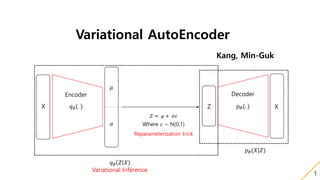
  • 1. Variational AutoEncoder Kang, Min-Guk 1 Z 𝑝 𝜃(. ) X Decoder X 𝑞∅(. ) Encoder 𝜇 𝜎 𝑍 = 𝜇 + 𝜎𝜀 Where 𝜀 ~ N(0,1) Reparameterization trick 𝑞∅ 𝑍 𝑋 Variational Inference 𝑝 𝜃(𝑋|𝑍)
  • 2. 1. 들어가기 앞서 알고 있으면 좋은 지식 2 1. Manifold Manifold란 두 점 사이의 거리 혹은 유사도가 근거리에서는 Euclidean metric을 따르지만 원거리에서는 그렇지 않은 공간을 의미한다. 2. Manifold Hypothesis 1. 고차원의 data 밀도는 낮지만, 이들의 집합을 포함하는 저차원의 Manifold가 있다. 2. 이 저차원의 Manifold를 벗어나는 순간 급격히 밀도는 낮아진다. → 우리의 고차원 데이터(Mnist의 경우 784차원)를 저차원 Manifold로 차원감소를 시키면, 데이터의 분포가 조밀해지고 데이터를 서로 비교할 수 있는 Boundary가 생긴다.
  • 3. 1. 들어가기 앞서 알고 있으면 좋은 지식 3 고차원의 MNIST 데이터 VAE를 이용해 차원감소를 시킨 2D- MNIST 데이터
  • 4. 1. 들어가기 앞서 알고 있으면 좋은 지식 4 첫 번째 사진과 세 번째 사진의 중간을 찾고 싶을 때는 유클리디안 거리를 이용하면 안된다! 자료 출처: https://www.facebook.com/groups/TensorFlowKR/permalink/496009234073473/?hc_location=ufi 다운로드: https://mega.nz/#!tBo3zAKR!yE6tZ0g-GyUyizDf7uglDk2_ahP-zj5trVZSLW3GAjw (Hwalsuk Lee님 슬라이드 자료에서 따왔습니다.)
  • 5. 1. 들어가기 앞서 알고 있으면 좋은 지식 5 Manifold 공간 상 중간에 있는 값을 사용해야 좋은 예측을 할 수 있다! 자료 출처: https://www.facebook.com/groups/TensorFlowKR/permalink/496009234073473/?hc_location=ufi 다운로드: https://mega.nz/#!tBo3zAKR!yE6tZ0g-GyUyizDf7uglDk2_ahP-zj5trVZSLW3GAjw (Hwalsuk Lee님 슬라이드 자료에서 따왔습니다.)
  • 6. 1. 들어가기 앞서 알고 있으면 좋은 지식 6 3. Bayes Rule 𝑃 𝑋 𝑌 = 𝑃(𝑌|𝑋)𝑃(𝑋) 𝑃(𝑌) 4. KL-Divergence 𝐷 𝐾𝐿 𝑃 𝑄 = 𝑖 𝑝 𝑖 𝑙𝑜𝑔 𝑃 𝑖 𝑄 𝑖 두 확률 분포 P, Q사이의 유사도를 측정하는 방법으로, 값이 작을 수록 두 확률분포가 유사하며, 항상 0보다 큰 특징을 가지고 있다. likelihood prior Normalize term posterior
  • 7. 2. Variational AutoEncoder 우리의 목표는 Normal distribution N(0,1) 에서 Z를 샘플링을 한 후 이를 이용하여 X라는 데이터를 생성하는 것이다. 즉 그림으로 표현을 하면 아래와 같다. N(0,1) ~ Z 𝑝 𝜃(𝑋|𝑍) X Decoder 𝑝 𝜃(𝑋|𝑍)를 Gaussian distribution으로 가정하게 되면 이 문제는 p x = 𝑝 𝑥 𝑔 𝜃 𝑧 𝑝(𝑧)𝑑𝑧를 최대화 해주는 MLE문제가 된다. 하지만, 7
  • 8. 2. Variational AutoEncoder 위의 논문에도 나와있듯 P(X|Z)를 Gaussian distribution으로 가정하고, -log(P(X))를 Minimize 할 시 데이터 사이의 Euclidian distance가 작아지도록 학습이 일어나 학습이 정확한 방향으로 되지 않는다. Figure 3의 (a)라는 데이터를 이용해 학습을 했다고 하면 (c)라는 결과가 나와야 좋은데, Euclidian distance가 가까운 (b)가 생성된다. Tutorial on Variational Autoencoders : https://arxiv.org/pdf/1606.05908 8
  • 9. 2. Variational AutoEncoder 이를 해결하기 위해 Z를 무작정 N(0,1)에서 샘플링 하는 것이 아닌, 내가 가지고 있는 Input data X를 이용하여 Sampling을 한 것이 Variational AutoEncoder 이다. Z 𝑝 𝜃(. ) X Decoder X 𝑞 𝜃(. ) Encoder 9
  • 10. 2. Variational AutoEncoder 문제점 ① 𝑞 𝜃(𝑍|𝑋)를 계산 할 수 없음. Intractable함. → 𝑞∅(𝑍|𝑋)라는 확률분포를 정의해주고 KL-Divergence를 이용해 근사 시켜준다(Variational Inference). ② Backpropagation을 하려면 모델이 미분가능 해야 하는데 𝑞∅(𝑍|𝑋)는 미분 불가능하다. → Reparameterization Trick을 이용해 해결, 논문의 first contribution. Z 𝑝 𝜃(𝑋|𝑍) X Decoder X 𝑞 𝜃(𝑍|𝑋) Encoder 10
  • 11. 2. Variational AutoEncoder 11 문제점 ① 𝑞 𝜃(𝑍|𝑋)를 계산 할 수 없음. Intractable함. 아래의 cs231n slide 참조. 출처: http://cs231n.stanford.edu/
  • 12. 2. Variational AutoEncoder 12 문제점 ① 𝑞 𝜃(𝑍|𝑋)를 계산 할 수 없음. Intractable함. 아래의 cs231n slide 참조. → 𝑞∅(𝑋|𝑍)라는 확률분포를 정의해주고 KL-Divergence를 이용해 근사 시켜준다(Variational Inference). 𝑞∅(𝑍|𝑋)를 Gaussian distribution으로 가정하면, 우리의 네트워크는 아래와 같이 된다. Z 𝑝 𝜃(. ) X Decoder X 𝑞∅(. ) Encoder 𝜇 𝜎 N(𝜇,𝜎) ~
  • 13. 2. Variational AutoEncoder 13 이 부분이 문제! 문제점 ② Backpropagation을 하려면 모델이 미분가능 해야 하는데 𝑞∅(𝑍|𝑋)는 미분 불가능하다. → Reparameterization Trick을 이용해 해결, 논문의 first contribution. Z 𝑝 𝜃(. ) X Decoder X 𝑞∅(. ) Encoder 𝜇 𝜎 N(𝜇,𝜎) ~
  • 14. 2. Variational AutoEncoder 14 문제점 ② Backpropagation을 하려면 모델이 미분가능 해야 하는데 𝑞∅(𝑋|𝑍)는 미분 불가능하다. → Reparameterization Trick을 이용해 해결, 논문의 first contribution. Z 𝑝 𝜃(. ) X Decoder X 𝑞∅(. ) Encoder 𝜇 𝜎 𝑍 = 𝜇 + 𝜎𝜀 Where 𝜀 ~ N(0,1) Reparameterization trick
  • 15. 3. 수학(Maximum Marginal loglikelihood Estimation) 15 log 𝑃 𝜃 𝑋 = 1 × log 𝑃 𝜃 𝑋 = 𝑧 𝑃 𝜃 𝑍 𝑋 × log 𝑃 𝜃 𝑋 ≈ 𝑧 𝑞∅ 𝑍 𝑋 × log 𝑃 𝜃 𝑋 = 𝑧 𝑞∅ 𝑍 𝑋 × log 𝑃 𝜃 𝑋, 𝑍 𝑃 𝜃 𝑍 𝑋 = 𝑧 𝑞∅ 𝑍 𝑋 × log 𝑃 𝜃 𝑋, 𝑍 𝑞∅ 𝑍 𝑋 × 𝑞∅ 𝑍 𝑋 𝑃 𝜃 𝑍 𝑋 = 𝑍 𝑞∅ 𝑍 𝑋 × log 𝑃 𝜃 𝑋, 𝑍 𝑞∅ 𝑍 𝑋 + 𝑍 𝑞∅(𝑍|𝑋) × log( 𝑞∅ 𝑍 𝑋 𝑃 𝜃 𝑍 𝑋 ) 𝐾𝐿 − 𝐷𝑖𝑣𝑒𝑟𝑔𝑒𝑛𝑐𝑒의 정의에 의해 준 식은 다음과 같이 바뀐다. = 𝑍 𝑞∅ 𝑍 𝑋 × log 𝑃 𝜃 𝑋, 𝑍 𝑞∅ 𝑍 𝑋 + 𝐷 𝐾𝐿(𝑞∅(𝑍|𝑋)| 𝑃 𝜃 𝑍 𝑋 = 𝐿(𝑎) 𝜃, ∅; 𝑋 + 𝐷 𝐾𝐿(𝑞∅(𝑍|𝑋)| 𝑃 𝜃 𝑍 𝑋 … (1)
  • 16. 3. 수학(Maximum Marginal loglikelihood Estimation) 16 log 𝑃 𝜃 𝑋 = 𝑍 𝑞∅ 𝑍 𝑋 × log 𝑃 𝜃 𝑋, 𝑍 𝑞∅ 𝑍 𝑋 + 𝐷 𝐾𝐿(𝑞∅(𝑍|𝑋)| 𝑃 𝜃 𝑍 𝑋 = 𝐿(𝑎) 𝜃, ∅; 𝑋 + 𝐷 𝐾𝐿(𝑞∅(𝑍|𝑋)| 𝑃 𝜃 𝑍 𝑋 … (1) 위의 식의 𝐿(𝑎) 𝜃, ∅; 𝑋 부분을 조금만 더 전개해보자. 𝑍 𝑞∅ 𝑍 𝑋 × log 𝑃 𝜃 𝑋, 𝑍 𝑞∅ 𝑍 𝑋 = 𝑍 𝑞∅(𝑍|𝑋) × log( 𝑃 𝜃 𝑋, 𝑍 × 𝑃 𝜃 𝑍 𝑃 𝜃 𝑍 × 𝑞∅ 𝑍 𝑋 ) = 𝑍 𝑞∅(𝑍|𝑋) × log 𝑃 𝜃 𝑋, 𝑍 𝑃 𝜃 𝑍 − 𝑍 𝑞∅(𝑍|𝑋) × log 𝑞∅ 𝑍 𝑋 𝑃 𝜃 𝑍 = 𝑍 𝑞∅(𝑍|𝑋) × log 𝑃 𝜃 𝑋|𝑍 − 𝐷 𝐾𝐿(𝑞∅(𝑍|𝑋)| 𝑃 𝜃 𝑍 = 𝐿(𝑏) 𝜃, ∅; 𝑋 − 𝐷 𝐾𝐿(𝑞∅(𝑍|𝑋)| 𝑃 𝜃 𝑍 …(2) ∴ log 𝑃 𝜃 𝑋 = 𝐿(𝑎) 𝜃, ∅; 𝑋 + 𝐷 𝐾𝐿(𝑞∅(𝑍|𝑋)| 𝑃 𝜃 𝑍 𝑋 ≥ 𝐿(𝑎) 𝜃, ∅; 𝑋 이므로 Lower bound인 𝐿(𝑎) 𝜃, ∅; 𝑋 를 최대화 하면 log 𝑃 𝜃 𝑋 값도 최대가 된다고 생각할 수 있다.
  • 17. 3. 수학(Maximum Marginal loglikelihood Estimation) 17 log 𝑃 𝜃 𝑋 = 𝐿(𝑎) 𝜃, ∅; 𝑋 + 𝐷 𝐾𝐿(𝑞∅(𝑍|𝑋)| 𝑃 𝜃 𝑍 𝑋 ≥ 𝐿(𝑎) 𝜃, ∅; 𝑋 이므로 Lower bound인 𝐿(𝑎) 𝜃, ∅; 𝑋 를 최대화 하면 log 𝑃 𝜃 𝑋 값도 최대가 된다고 생각할 수 있다. 따라서 우리의 목표는 다음과 같이 다시 작성될 수 있다. 𝐴𝑟𝑔𝑚𝑎𝑥 𝜃 log 𝑃 𝜃 𝑋 ↔ 𝐴𝑟𝑔𝑚𝑎𝑥 𝜃,∅(𝐿 𝑎 𝜃, ∅; 𝑋 ) 𝐴𝑟𝑔𝑚𝑎𝑥 𝜃,∅ 𝐿 𝑎 𝜃, ∅; 𝑋 = 𝐴𝑟𝑔𝑚𝑎𝑥 𝜃,∅( 𝑍 𝑞∅ 𝑍 𝑋 × log 𝑃 𝜃 𝑋|𝑍 − 𝐷 𝐾𝐿(𝑞∅(𝑍|𝑋)| 𝑃 𝜃 𝑍 ) 위의 식에서 (b)는 𝑞∅(𝑍|𝑋)가 Gaussian distribution, 𝑃 𝜃 𝑍 가 Normal distribution이라고 할 때 다음과 같이 계산 가능하다. 𝐷 𝐾𝐿(𝑞∅(𝑍|𝑋)| 𝑃 𝜃 𝑍 = 1 𝑀 𝑖=1 𝑀 [ 1 2 𝑗=1 𝐷 {1 − log 𝜎𝑖,𝑗 2 + 𝜇𝑖,𝑗 2 + 𝜎𝑖,𝑗 2 }] Where D는 Data의 Dimension(MNIST의 경우 784), M은 데이터의 갯수 (a) (b)
  • 18. 3. 수학(Maximum Marginal loglikelihood Estimation) 18 𝐴𝑟𝑔𝑚𝑎𝑥 𝜃,∅ 𝐿 𝑎 𝜃, ∅; 𝑋 = 𝐴𝑟𝑔𝑚𝑎𝑥 𝜃,∅( 𝑍 𝑞∅ 𝑍 𝑋 × log 𝑃 𝜃 𝑋|𝑍 − 𝐷 𝐾𝐿(𝑞∅(𝑍|𝑋)| 𝑃 𝜃 𝑍 ) (a)의 경우, 아래와 같은 방법으로 계산하면 결론적으로 Cross_entropy와 같은 결과를 얻게 된다. 𝑍 𝑞∅ 𝑍 𝑋 × log 𝑃 𝜃 𝑋|𝑍 ≈ 1 𝐿 𝑍 𝑙= 𝑍1 𝑧 𝐿 log( 𝑃 𝜃 𝑋|𝑍𝑙 … 𝑏𝑦 𝑀𝑜𝑛𝑡𝑒 𝑐𝑎𝑟𝑙𝑜 𝑡𝑒𝑐ℎ𝑛𝑖𝑞𝑢𝑒 편의를 위해 L =1이라고 가정하면 준식 = log(𝑃 𝜃 𝑋 𝑍1 가 된다. X의 Dimension을 D라고 가정하고, data의 수를 M이라 가정했을 시 아래와 같이 전개할 수 있다. log(𝑃 𝜃 𝑋 𝑍1 = 1 𝑀 𝑖=1 𝑀 log 𝑗=1 𝐷 𝑃 𝜃 𝑋𝑖,𝑗 𝑍1 = 1 𝑀 𝑖=1 𝑀 𝑗=1 𝐷 log 𝑃 𝜃 𝑋𝑖,𝑗 𝑍1 𝑃 𝜃 𝑋𝑖,𝑗 𝑍1 를 Bernoulli distribution이라 가정했을 시 위 식은 아래와 같이 전개 가능하다. = 1 𝑀 𝑖=1 𝑀 𝑗=1 𝐷 log 𝑃𝑖,𝑗 𝑋 𝑖,𝑗 (1 − 𝑃𝑖,𝑗)(1−𝑋 𝑖,𝑗) = 1 𝑀 𝑖=1 𝑀 𝑗=1 𝐷 {𝑋𝑖,𝑗log 𝑃𝑖,𝑗 + 1 − 𝑋𝑖,𝑗 𝑙𝑜𝑔(1 − 𝑃𝑖,𝑗)} … 𝐶𝑟𝑜𝑠𝑠 𝐸𝑛𝑡𝑟𝑜𝑝𝑦 𝐸𝑞𝑢𝑎𝑡𝑖𝑜𝑛. (a) (b)
  • 19. 3. 수학(Maximum Marginal loglikelihood Estimation) 19 따라서 앞의 두 슬라이드에서 계산했듯이 𝐴𝑟𝑔𝑚𝑎𝑥 𝜃,∅ 𝐿 𝑎 𝜃, ∅; 𝑋 = 𝐴𝑟𝑔𝑚𝑎𝑥 𝜃,∅( 𝑍 𝑞∅ 𝑍 𝑋 × log 𝑃 𝜃 𝑋|𝑍 − 𝐷 𝐾𝐿(𝑞∅(𝑍|𝑋)| 𝑃 𝜃 𝑍 ) 이 문제는 아래의 값의 최대 값을 구하는 문제와 동치이게 된다. 𝐿 𝑎 𝜃, ∅; 𝑋 = 1 𝑀 𝑖=1 𝑀 𝑗=1 𝐷 {𝑋𝑖,𝑗log 𝑃𝑖,𝑗 + 1 − 𝑋𝑖,𝑗 𝑙𝑜𝑔(1 − 𝑃𝑖,𝑗)} − 1 𝐿 𝑖=1 𝐷 [ 1 2 𝑗=1 𝐽 {1 − log 𝜎𝑖,𝑗 2 + 𝜇𝑖,𝑗 2 + 𝜎𝑖,𝑗 2 }] Fully convolutional network에서는 Gradient Descent Algorism을 사용하므로 −𝐿 𝑎 𝜃, ∅; 𝑋 = − 1 𝑀 𝑖=1 𝑀 𝑗=1 𝐷 {𝑋𝑖,𝑗log 𝑃𝑖,𝑗 + 1 − 𝑋𝑖,𝑗 𝑙𝑜𝑔(1 − 𝑃𝑖,𝑗)} + 1 𝐿 𝑖=1 𝐷 [ 1 2 𝑗=1 𝐽 {1 − log 𝜎𝑖,𝑗 2 + 𝜇𝑖,𝑗 2 + 𝜎𝑖,𝑗 2 }] 값을 최소화 시키는 파라미터들을 학습 시켜주면 된다.
  • 20. 4. 코드로 보는 Gaussian_encoder 20 def gaussian_encoder(X, n_hidden, n_z, keep_prob): w_init = tf.contrib.layers.xavier_initializer() input_shape = X.get_shape() with tf.variable_scope("encoder_hidden_1", reuse = tf.AUTO_REUSE): w1 = tf.get_variable("w1", shape = [input_shape[1], n_hidden], initializer = w_init) b1 = tf.get_variable("b1", shape = [n_hidden], initializer = tf.constant_initializer(0.)) h1 = tf.matmul(X,w1) + b1 h1 = tf.nn.elu(h1) h1 = tf.nn.dropout(h1, keep_prob) with tf.variable_scope("encoder_hidden_2", reuse = tf.AUTO_REUSE): w2 = tf.get_variable("w2", shape = [n_hidden,n_hidden], initializer = w_init) b2 = tf.get_variable("b2", shape = [n_hidden], initializer = tf.constant_initializer(0.)) h2 = tf.matmul(h1,w2) + b2 h2 = tf.nn.elu(h2) h2 = tf.nn.dropout(h2,keep_prob) with tf.variable_scope("encoder_z", reuse = tf.AUTO_REUSE): w3 = tf.get_variable("w3", shape = [n_hidden, n_z*2], initializer = w_init) b3 = tf.get_variable("b3", shape = [n_z*2], initializer = tf.constant_initializer(0.)) h3 = tf.matmul(h2,w3) + b3 mean = h3[:, : n_z] std = tf.nn.softplus(h3[:, n_z :]) + 1e-6 return mean, std 슬라이드 17번에서 KL_Divergence계산을 위해 𝑞∅(𝑍|𝑋)가 Gaussian distribution라고 가정하였음.
  • 21. 4. 코드로 보는 Bernoulli_decoder 20 def Bernoulli_decoder(z, n_hidden, n_out ,keep_prob): w_init = tf.contrib.layers.xavier_initializer() z_shape = z.get_shape() with tf.variable_scope("decoder_hidden_1", reuse = tf.AUTO_REUSE): w4 = tf.get_variable("w4", shape = [z_shape[1],n_hidden], initializer = w_init) b4 = tf.get_variable("b4", shape = [n_hidden], initializer = tf.constant_initializer(0.)) h4 = tf.matmul(z,w4) + b4 h4 = tf.nn.elu(h4) h4 = tf.nn.dropout(h4,keep_prob) with tf.variable_scope("decoder_hidden_2", reuse = tf.AUTO_REUSE): w5 = tf.get_variable("w5", shape = [n_hidden, n_hidden], initializer = w_init) b5 = tf.get_variable("b5", shape = [n_hidden], initializer = tf.constant_initializer(0.)) h5 = tf.matmul(h4,w5) + b5 h5 = tf.nn.elu(h5) h5 = tf.nn.dropout(h5, keep_prob) with tf.variable_scope("decoder_output", reuse = tf.AUTO_REUSE): w6 = tf.get_variable("w6",shape = [n_hidden, n_out], initializer = w_init) b6 = tf.get_variable("b6", shape = [n_out], initializer = tf.constant_initializer(0.)) h6 = tf.matmul(h5,w6) + b6 h6 = tf.nn.sigmoid(h6) return h6 슬라이드 18번에서 𝑍 𝑞∅ 𝑍 𝑋 × log 𝑃 𝜃 𝑋|𝑍 계산을 위해 𝑃 𝜃 𝑋𝑖,𝑗 𝑍1 를 Bernoulli distribution 라고 가정하였음.
  • 22. 4. 코드로 보는 Variational autoencoder 20 def Variational_autoencoder(X,n_hidden_encoder,n_z, n_hidden_decoder, keep_prob ): X_shape = X.get_shape() n_output = X_shape[1] mean, std = gaussian_encoder(X,n_hidden_encoder, n_z,keep_prob) z = mean + std*tf.random_normal(tf.shape(mean,out_type = tf.int32), 0, 1, dtype = tf.float32) X_out = Bernoulli_decoder(z,n_hidden_decoder,n_output,keep_prob) X_out = tf.clip_by_value(X_out,1e-8, 1 - 1e-8) likelihood = tf.reduce_mean(tf.reduce_sum(X*tf.log(X_out) + (1-X)*tf.log(1- X_out),1)) KL_Divergence = tf.reduce_mean(0.5*tf.reduce_sum(1 - tf.log(tf.square(std) + 1e-8) + tf.square(mean) + tf.square(std), 1)) Recon_error = -1*likelihood Regularization_error = KL_Divergence ELBO = Recon_error + Regularization_error return z ,X_out, Recon_error, Regularization_error, ELBO Encoder와 Decorder를 사용해서 Variational autoencoder를 작성하였음.
  • 23. 4. 코드로 보는 Optimization 20 likelihood = tf.reduce_mean(tf.reduce_sum(X*tf.log(X_out) + (1-X)*tf.log(1- X_out),1)) KL_Divergence = tf.reduce_mean(0.5*tf.reduce_sum(1 - tf.log(tf.square(std) + 1e-8) + tf.square(mean) + tf.square(std), 1)) Recon_error = -1*likelihood Regularization_error = KL_Divergence ELBO = Recon_error + Regularization_error optimizer = tf.train.AdamOptimizer(learning_rate = learning_rate_decayed).minimize(ELBO)
  • 24. 5. ELBO함수의 의미 21 −𝐿 𝑎 𝜃, ∅; 𝑋 = 𝑍 𝑞∅ 𝑍 𝑋 × log 𝑃 𝜃 𝑋|𝑍 − 𝐷 𝐾𝐿(𝑞∅(𝑍|𝑋)| 𝑃 𝜃 𝑍 Reconstruction Error AutoEncoder 관점에서 본 X에 대한 복원오차 Regularization 주어진 데이터로 부터 Z를 잘 샘플링 했는지를 나타내는 척도
  • 25. 6. 전체 모델 22 Z 𝑝 𝜃(. ) X Decoder X 𝑞∅(. ) Encoder 𝜇 𝜎 𝑍 = 𝜇 + 𝜎𝜀 Where 𝜀 ~ N(0,1) Reparameterization trick 𝑞∅ 𝑍 𝑋 Variational Inference 𝑝 𝜃(𝑋|𝑍)
  • 26. 7. 결과 23 중간에 샘플링 하는 부분이 있기 때문에 이미지가 흐릿하게 생성된다.
  • 27. 7. 결과 24 Input X에 대한 𝜇와 𝜎를 각각 2개씩 Neural network를 이용하여 뽑은 후 이를 이용하여 Z를 샘플링 한다. [None,2]의 모양을 가진 Z를 Z[:,0]를 X축, Z[:,1]를 Y축으로 하여 그래프를 그리면 옆의 사진과 같은데, 이를 보면 앞의 슬라이드 2페이지에서 말했던 Manifold Hypothesis를 눈으로 직접 확인 할 수 있다.
  • 28. 7. 결과 25 바로 이전 슬라이드의 그래프에서 X를 -2~2까지 균등하게 Y를 -2~2까지 균등하게 뽑은 후 이 두 값을 이용하여 2-Dimension Z 를 만들고 생성모델 P(X|Z)을 이용해 X를 생성하면 옆의 그림과 같은 2-D manifold를 직접 확인 할 수 있다.