Zwaan Eage 2004 V3
•Transferir como DOC, PDF•
0 gostou•471 visualizações

AVO friendly processing - Geophysics

Recomendados
Recomendados
Mais conteúdo relacionado
Mais procurados
Mais procurados (20)
Semelhante a Zwaan Eage 2004 V3
Semelhante a Zwaan Eage 2004 V3 (20)
Último
Último (20)
Zwaan Eage 2004 V3
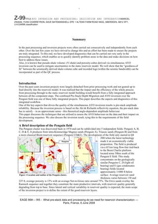
- 1. 1 Z-99 TITLE AVO INVERSION AND PROCESSING: DEDICATION AND INTEGRATIONMARCEL ZWAAN, YVAN CHARREYRON, DAVE BATEMANSHELL EPE 1 ALTENS FARM ROAD NIGG, ABERDEEN, AB12 3FY, U.K.EAR99 classification Summary In the past processing and inversion projects were often carried out consecutively and independently from each other. Over the last few years we have strived to change this and an effort has been made to ensure the projects are truly integrated. To this end, we have developed diagnostics that can be carried out very early in the processing sequence, which enables us to quickly identify problem areas in the data and make decisions on how best to address these issues. Also, it is known that pseudo-shale volume- (V-shale) and porosity-cubes derived via simultaneous AVO inversion can be used to mitigate uncertainties in the static reservoir model. We will show that the “goodness-of fit” between the seismically derived shale-volume cube and recorded logs (within the seismic bandwidth) can be incorporated as part of the QC process. Introduction Over the past years inversion projects were largely detached from prior processing work and not geared up to feed directly into the reservoir model. It was realised that the impact and the efficiency of the whole process from processing through to the static reservoir model building would benefit from a fully integrated approach between all the component steps. The combined Pre-Stack Depth Migration and AVO inversion over the Penguin field was one of these fully integrated projects. This paper describes the aspects and diagnostics of this integrated workflow. One of the key aspects that drives the quality of the simultaneous AVO inversion results is pre-stack amplitude reliability. Because the inversion process is based on the Aki & Richards reflectivity equation, the pre-stack data has to satisfy – in an approximate sense - this theoretical angle-dependent amplitude behaviour. This paper discusses the techniques that are utilised to assess the AVO behaviour on the data and their impact on the processing sequence. We also discuss the inversion result, tying this to the requirements of the field development. A Brief description of the Penguin field The Penguin cluster was discovered back in 1974 and can be subdivided into 5 independent fields: Penguin A, B, C, D & E. It produces from intra-Kimmeridge Magnus sands (Penguin A), Triassic sands (Penguin B) and from a more classical Brent reservoir sequence (Penguin CD&E). The development of the field only started in Q4 2001when the latest technology Penguins made it an economically viable proposition. The field is produced via a 65 km long flow-line tied-back to the Brent Charlie platform located some 50km south of the Penguin E field. This study concentrates on the geologically similar Penguins C, D (light oil bearing) and E (gas condensates bearing) fields located approximately 11000 ft below Figure 1 Location and outline of the Penguin cluster. surface. Average reservoir sand thickness varies between 130 and 225 ft, average porosity is 15% with an average Net-to-Gross ratio around 75%. The Etive sands overlay the Rannoch sequence and together they constitute the main productive intervals, with reservoir quality generally degrading from top to base. Since lateral and vertical variability in reservoir quality is expected, the main scope of the inversion project is to define the extent of the good reservoir layers. EAGE 66th – W5 - What pre-stack data and processing do we need for reservoir characterization — Paris, France, 6 June 2004
- 2. 2 Project planning and inversion feasibility Because of the field’s structural complexity, it was decided that a Pre-Stack Depth Migration (PreSDM) was to be carried out over the Penguin cluster. In the planning of the processing and inversion sequence, the AVO feasibility step was started at the beginning of the PreSDM velocity model updating cycle, in order to be able to impact the final migration result prior to inversion. Therefore the feasibility study and the velocity model updating were carried out in parallel. At the start of the project - in parallel to the seismic data processing - P- and S-sonic logs and density logs were edited, and corrected for borehole invasion effects. Then, Gassmann fluid substitution was performed and the resulting brine, oil and gas(-condensate) bearing logs were used to model AVO synthetic seismic from which it became apparent that no reliable hydrocarbon indicator was likely to be found. However, cross-plot analysis including reservoir-sand and overlying shale sequences showed that there was scope for lithology separation in the Ip-Is domain. Therefore the main target of the inversion workflow became facies identification and subsequently identification of high porosity sand units. Avo Diagnostics Two types of AVO diagnostics were carried out, and both methods will be described here in more detail. The first method is a diagnostic applied to pre-stack data, which are in this case the common image gathers obtained from Pre-Stack Depth Migration. The second diagnostic is a sub-stack diagnostic, applied to the near mid and far angle stacks. The first method, pertaining to pre-stack common image gathers identifies problems with the fit of the two-term Aki and Richards equation to the amplitudes of this pre-stack data: A(θ ) = L + M sin 2 θ . The above two terms are commonly known as intercept and gradient. This two-term equation is fitted to the events on common image gathers. (The velocities employed in the migration yield the time variant offset versus angle relations.) Subsequently, for each angle, a Figure 2 RMS of the Near Mid and Far error cubes Obtained by “synthetic” amplitude is computed from the above a gated measurement over the top Brent horizon equation, which can then be subtracted from the observed seismic amplitude. In this manner an “error” value can be obtained, for every time sample, at every angle (cf. “Making AVO Sections More Robust” by Andrew Walden, BP, 52nd EAGE Meeting Copenhagen, 1990). This error is squared and is then summed for each sub-stack angle range to obtain an average error pertaining to the near, mid and far angle ranges, respectively. Note that in this manner we have obtained three cubes of data (for the near, mid and far angle ranges) that contains an average error over each of the angle range for every time sample. After taking the square root, the rms-error can be viewed either as a volume, or alternatively rms-error horizons can be extracted, e.g. in time gates around key horizons. In a schematic view the error computation can work like this: Amplitude vs. error vs. angle angle Figure 2 shows the rms- Figure 3 error maps computed Image gathers Image from the near mid and far “error” cubes, respectively. These maps have been obtained from a windowed measure- ment along the top reservoir horizon (see Fig. 3, yellow marker indicates the top Brent pick) with the blue colour indicating high error. These maps provide a quick tool to Figure 3 Image Gathers (left) with indications of multiples, and residual move out Stacked image gathers (right) with X-unconformity (red), top Brent (yellow) and top Dunlin (green)
- 3. 3 locate the areas of high error, allowing the common image gathers and their corresponding stack to be inspected to identify the potential cause of these large misfits. The common image gathers and a migrated stack are displayed in Fig. 3, to illustrate the usefulness of this diagnostic. Some of the gathers indeed show problematic behaviour (arrows in Fig. 3). Residual move-out is also visible, but that is not yet important at this stage, as this first depth migration only uses an initial velocity model. By contrast, much more important are the suspected multiples over the reservoir section. This diagnostic allowed us to identify very early in the processing the requirement that a further multiple removal application on the final volume migrated output would be necessary. The products on input to the simultaneous AVO inversion are the near, mid and far angle stacks. The standard pre-inversion processing procedure comprises the alignment of Figure 4 Near Mid and Far stacks. The amplitudes become stronger the different angle stacks and a from near to mid, and then drop again from the mid to far stack. This area was spectral shaping of the near and far identified by means of the sign-flip diagnostic. stacks towards the spectral character of the mid angle stack. For this data, the spectral balancing was preceded by two multiple removal steps, a (pre-stack) tau-p decon- volution over the reservoir section, and a further post-stack multiple removal deeper down on each of the angle stacks so as not to affect the amplitude behaviour over the reservoir. After this processing stage, the second type of AVO diagnostic can be run. This is a post-stack diagnostic that consists in a repeated fit of the two-term Aki and Richards equation to the sub-stacks. Firstly, a fit to the near and mid sub-stacks delivers the first set of intercept and gradient values, followed by a fit to the near and the far, that delivers a second set of intercept and gradient values. It is generally known that the computed gradient values will display much lower signal to noise levels than the intercept (which indeed only shows small variation in both fits), but on the other hand, a high level of accuracy of the gradient term is not required for the diagnostic computed here. Actually the only aspect that we are really interested in is a change of sign of “large” gradient terms: M 2 − M1 S = 200sign( M 1 ) sign( M 2 ) . M1 + M 2 Figure 4 illustrates this gradient difference map with an arrow indicating an area where the gradient sign-flip occurs (when S is negative). The near, mid and far angle stacks are also shown, with the area of the gradient sign change indicated by the ellipses over the sections. The conclusion that can be drawn from this post-stack diagnostic is based on the fact that these identified problem areas are very limited in extent. Because these “noisy” areas don’t seem to represent an extensive problem the overall conclusion made from these diagnostics is that an AVO inversion would provide reliable and sensible results. Further QC’s were carried out on the stacks prior to the inversion. These diagnostics assessed: data alignment, multiple removal, and the spectral balancing. An AVO inversion with Jason software was performed, producing P- and S-impedance cubes. Based on the Figure 5 Well logs (green) and V-shale cube (red) compared at the 142S1 and 141S2 wells rock-physics model, a shale-fraction cube and a porosity cube were derived from these Ip and Is volumes. Inversion results Raw inversion products, as well as derived V-shale and porosity cubes were QC-ed against well measurements. In order to assess AVO information only, both cubes and well logs were filtered back to the seismic bandwidth. The “goodness of fit” between band-limited logs and derived cubes is observed to be generally good as EAGE 66th – W5 - What pre-stack data and processing do we need for reservoir characterization — Paris, France, 6 June 2004
- 4. 4 illustrated in Figure 5. Furthermore, in order to assess the potential added value of the inversion products, they were compared with the existing reservoir model. In comparing porosity maps (see Fig.6), it can be seen that average trends are very similar, but the seismically derived products may deliver additional information that is not yet captured in the current model. These results still need further evaluation before they could be used to constrain higher resolution lithology and porosity cubes of the static reservoir model. An alternative manner to evaluate inversion results consists in looking at the horizontal wells that were not included in the low-frequency Figure 6 Porosity column from the reservoir model (left) compared with the one of the inverted cube (right). The inversion result sows more detail at several locations. inversion background model. In this respect, the C2 and D1 production wells were not incorporated in the inversion workflow, and therefore they represent good reliable blind tests. As shown in Figure 7, the C2 well encountered a thin up-thrown shale block within the reservoir interval, that had never been spotted on reflection seismic, but which was correctly indicated on the V-shale section of the inverted result. Similarly, when compared to the D1 logs, the V-shale cube derived from the inversion showed a good match. This included the identification of a sand body at the toe of the well that was poorer quality than expected from the reflectivity data. Due to the varying thickness of the overlaying Humber group (Kimmeridge and Heather shales), the top Brent pick Figure 7 The horizontal C2 well (not indicated) encountered an up-thrown shale block in the reservoir section. The vertical 211/13-2 well (indicated) shows a very thin cannot easily be interpreted accurately on Kimmeridge section of approximately 30 ft. The V-shale cube from the inversion ties reflectivity data, as it can be masked by the well log very well over the reservoir section. the side-lobe energy from the much stronger contrast at Base Cretaceous unconformity level. Because of the broader bandwidth of the inversion result that tends to minimize tuning effects, the resultant cubes also offer the possibility for refining top-reservoir interpretation for increased volumetric accuracy. Conclusion The two AVO diagnostics, a pre-stack and a post-stack AVO diagnostic, discussed in this paper have proven to be successful during this integrated project, and have impacted the processing sequence to optimize the inversion result. Subsequently, we showed that the inversion cubes exhibit some very positive features that have been confirmed by “blind well” results. Further evaluation of the inversion-data is needed before it – or part of it is included in the reservoir model. Finally, the AVO diagnostics presented here have made an important contribution to the integration of the several components of this combined PreSDM - AVO inversion project. Acknowledgements: The authors would like to thank Exxon-Mobil and Shell EP Europe for their kind permission to publish this material. Moreover, we want to thank several of our colleagues who contributed to the development of the AVO diagnostics, Peter Ashton, Greg Hester, Henk Tijhof and Peter Rowbotham. Furthermore, we want to mention in particular Alexander Sementsov and Richard Shipp for their work on the inversion and PreSDM, respectively.