
Recomendados
Mais conteúdo relacionado
Mais procurados
Mais procurados (20)
Destaque
Destaque (20)
Semelhante a Thesis defense
Semelhante a Thesis defense (20)
Último
Último (20)
Thesis defense
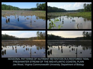
- 1. SEASONAL PATTERNS OF NUTRIENT RETENTION IN A RESTORED TIDAL FRESHWATER STREAM OF THE MID-ATLANTIC COASTAL PLAIN Joe Wood, Virginia Commonwealth University, Department of Biology
- 2. Outline • Nutrient transport and associated problems • Description of Tidal Freshwater Systems • Site Description & Project Goals • Methods • Results • Conclusions and implications
- 3. What are Nutrients? •Elements whose environmental supply is low in relation to biological demand (N, P) •Small amounts of nutrients can result in large responses from biotic systems.
- 4. Exponential Increase in Nutrient Transport By watersheds Stimulated Algae Production Decomposition of Algae Depletes Dissolved Oxygen, Eutrophication
- 5. Watershed-scale budgets Basic Terminology •Sources vs. Sinks •Inorganic (NH4,NO3) vs. Organic forms •Assimilation vs. mineralization •De-nitrification
- 6. Tidal Freshwater Systems “Along the hydrologic continuum between streams and ocean lies a unique ecotone where river meets estuary” Ensign et al 2008 •These systems are ecologically distinct from both non-tidal streams and salt marshes but have been understudied. Gravity Tides Fresh Water Salt Headwaters Tidal Freshwater Oceans
- 7. Why are Tidal Freshwater Streams “biogeochemical hotspots”? 1. Increased exposure to active surfaces (benthic layer) 2. Diverse chemical and physical habitats (anaerobic zones, floodplains) 3. Higher Organic Matter availability (Neubauer et al 2009)
- 8. Ecosystem Metabolism Photosynthesis: CO2 + H2O + Light CxH2xOx + O2 Respiration: Gross Primary Production = CxH2xOx + O2 CO2 + H2O total amount of energy (or C) fixed via photosynthesis per unit of time. How do these parameters influence Ecosystem Respiration= Nutrient Retention? total amount of energy (or C) used via respiration per unit time.
- 9. . Seasonal Variation Primary Production Respiration Exchange Volume Ambient Nutrient levels Mass Nutrient Retention
- 10. Project Goals • Characterize Annual nutrient Budgets for a recently restored tidal freshwater stream. • Estimate seasonal variation in Ecosystem Metabolism (using diel dissolved oxygen patterns). • Determine controlling factors of nutrient retention.
- 11. Methods • Site Description • Tidal exchange sampling method • Characterizing Hydrology with rhodamine • Nutrient additions • Estimating Ecosystem Metabolism
- 12. Until September 2006 When a breach occurred in the dam in Kimages Creek Was dammed causing to formDrawdown, and 1927 Lake lake Charles reconnecting tidal inputs to Kimages creek. This narrow breach provides the ability to measure all exchange between Kimages Creek and the James River.
- 13. Sampling Regime Q = Discharge (L/s) X = Solute Concentration (mg/L) QntXnt Qtidal , Xtidal Qout, Xout X = Cl, NO3, NH4, TN, PO4, TP and DOC Head of tide
- 14. Non-tidal input Stream Cl input River Cl input Chloride should behave conservatively, thus producing un-altered outflows. A Conservative Tracer (Chloride) Tidal Exchange
- 15. Stream input Non-tidal input chemistry River input chemistry Retained Nitrogen A Non-Conservative Tracer (Nutrients) Tidal Exchange
- 16. Characterizing Hydrology Rhodamine Additions (2) on a Rising Tide.
- 17. Nutrient Additions (3) Raised ambient NH4 and PO4 nutrient levels by roughly 20%
- 18. Measuring Ecosystems Metabolism 16 DARK LIGHT 15 (R) (PS + R) 14 DO eq (mg/L) 13 12 11 10 9 8 0:00 9:30 19:00 4:30 14:00 23:30 9:00 18:30 4:00 13:30 23:00 Photosynthesis: CO2 + H2O + Light CxH2xOx + O2 Respiration: CxH2xOx + O2 CO2 + H2O We Must also account for Atmospheric Exchange…
- 19. Atmospheric Exchange Oxygen To estimate Atmospheric Exchange (AE) we used a method which assumes a constant boundary layer thickness. Thus AE is only influenced by Depth and Difference in Saturation.
- 20. Advective influences 12 0.08 DO 10 Depth 0.06 8 O2 (mg/L) Depth (m) 6 0.04 4 0.02 2 0 0.00 During certain times of the year when oxygen concentrations were drastically different between sources, Kimages displayed advective influences of Oxygen.
- 21. Results • Water • Nutrient • Annualized Budgets • Metabolism Estimates • High Flow events • Controlling factors of nutrient retention
- 22. Rhodamine Additions indicate this is a macro-tidal system Inflow Outflow Inflow 2.5 Rhodamine Flux (g/min) I 2 n j 1.5 e c 1 t i 0.5 o n 96,80% 0 0 2 4 6 8 10 12 14 16 18 Time since rhodamine injection (hours)
- 23. Average Water Fluxes 8000 1500 3500 (Storage) 13000 All Units in M3/ Tidal Cycle
- 24. 40000 Water Fluxes 0.4 35000 Gloucester Point James River 0.2 Volume of Exchange (m3) 30000 0 Water Stage (m) 25000 20000 -0.2 15000 -0.4 10000 -0.6 5000 0 -0.8 In Out In Out In Out In Out In Out In Out In Out In Out In Out In Out In Out In Out Sep Oct Nov Dec Jan Feb Mar Apr May Jun Jul Aug Storage Tidal output Tidal Input Non-tidal input 60000 50000 Exchange volume (m3) R² = 0.78 40000 30000 20000 10000 0 0.0 0.5 1.0 1.5 2.0 2.5 3.0 River depth (m)
- 25. Predicted Outflow - Actual outflow Predicted Outflow - Actual outflow (NH3 mg/L) NH4 (mg/L) NO3 (mg/L) (NOx mg/L) (mg/L) Cl Outflow (mg/L) Measured Cl -0.10 -0.05 -0.25 -0.20 -0.15 0.00 0.05 0.10 0.02 0.00 0.04 -0.06 -0.02 -0.12 -0.10 -0.08 -0.04 0 10 20 30 60 70 40 50 0 S 9/24/2008 10 O 10/24/2008 20 P = 0.0000 D R² = 0.9909 12/9/2008 30 J 1/18/2009 40 F 2/21/2009 Predicted Cl (mg/L) 50 60 M 3/21/2009 Cl Inflow (mg/L) 1:1 70 A 4/25/2009 M 5/19/2009 J 6/19/2009 J 7/31/2009 A 8/19/2009 Predicted Outflow - Actual outflow Predicted Outflow - Actual outflow TN (mg/L) (TN mg/L) TON (mg/L) (TON mg/L) -0.150 -0.100 -0.050 -0.250 -0.200 0.000 0.050 0.100 -0.10 -0.05 -0.20 -0.15 0.00 0.05 0.10 S 9/24/2008 O 10/24/2008 D 12/9/2008 J 1/18/2009 F 2/21/2009 RELEASE M differences 3/21/2009 A 4/25/2009 M 5/19/2009 J 6/19/2009 J RETENTION 7/31/2009 Nutrient Concentration A 8/19/2009
- 26. Chloride Fluxes 1,600,000 1,400,000 Delta Storage 1,200,000 Total output 1,000,000 Tidal g cl Flux/Tidal Cycle 800,000 Non-tidal 600,000 400,000 200,000 0 In Out In Out In Out In Out In Out In Out In Out In Out In Out In Out In Out Sep Oct Dec Jan Feb Mar Apr May Jun July Aug
- 27. Inorganic Nitrogen Fluxes 7,000 "Change in Storage" 6,000 Total output g NOx Flux/Tidal Cycle 5,000 "Change in Storage" g NO3 4,000 Tidal Total output Tidal 3,000 Non-tidal Non-tidal 2,000 1,000 0 2,500 In Out In Out In Out In Out In Out In Out In Out In Out In Out In Out In Out Sep Oct Dec Jan Feb Mar Apr May Jun July Aug 2,000 In Out In Out In Out In Out In Out In Out In Out In Out In Out g NH4 Flux/Tidal Cycle g NH4 1,500 Dec Jan Feb Mar Apr May Jun July Aug 1,000 500 0 In Out In Out In Out In Out In Out In Out In Out In Out In Out In Out In Out Sep Oct Dec Jan Feb Mar Apr May Jun July Aug
- 28. 30,000 25,000 "Change in Storage" g DIN Flux/Tidal Cycle 20,000 Total output g DIN 15,000 10,000 Tidal Non-tidal 5,000 0 30,000 In Out In Out In Out In Out In Out In Out In Out In Out In Out In Out In Out 25,000 Sep Oct Dec Jan Feb Mar Apr May Jun July Aug g TON Flux/Tidal Cycle 20,000 g TON 15,000 n Out In Out In Out In Out In Out In Out In Out In Out In Out 10,000 Dec Jan 5,000 Feb Mar Apr May Jun July Aug 0 30,000 In Out In Out In Out In Out In Out In Out In Out In Out In Out In Out In Out Sep Oct Dec Jan Feb Mar Apr May Jun July Aug 25,000 g TN Flux/Tidal Cycle 20,000 g TN 15,000 10,000 5,000 0 In Out In Out In Out In Out In Out In Out In Out In Out In Out In Out In Out Sep Oct Dec Jan Feb Mar Apr May Jun July Aug
- 29. 1,800 1,600 "Change in Storage" 1,400 Total "Change in Storage" output g PO4 Flux/Tidal Cycle 1,200 g PO4 Total output 1,000 Tidal Tidal Non-tidal 800 Non-tidal 600 400 200 0 5,000 In Out In Out In Out In Out In Out In Out In Out In Out In Out In Out In Out 4,500 Sep Oct Dec Jan Feb Mar Apr May Jun Jul Aug 4,000 n Out In Out 3,500In Out In Out In Out In Out In Out In Out g TP Flux/Tidal Cycle 3,000 g TP Jan Feb 2,500 Mar Apr May Jun July Aug 2,000 1,500 1,000 500 0 300,000 In Out In Out In Out In Out In Out In Out In Out In Out In Out In Out In Out 250,000 Sep Oct Dec Jan Feb Mar Apr May Jun Jul Aug g DOC 200,000 g DOC Flux/Tidal Cycle 150,000 100,000 50,000 0 In Out In Out In Out In Out In Out In Out In Out In Out In Out In Out In Out Sep Oct Dec Jan Feb Mar Apr May Jun July Aug
- 30. Tracer 1600 Experiments ∆ Storage 1400 g NH4 /Tidal Cycle Injection 1200 1000 Output 800 Tidal 600 Non-tidal 400 200 0 2500 Inflow Outflow Inflow Outflow Inflow Outflow Inflow Outflow Inflow Outflow Inflow Outflow g PO4 /Tidal Cycle 2000 Ambient Injection Ambient Injection Ambient Injection May June August 1500 1000 500 0 Inflow Outflow Inflow Outflow Inflow Outflow Inflow Outflow Inflow Outflow Inflow Outflow Ambient Injection Ambient Injection Ambient Injection May June August
- 31. 3.0 a River Depth (m) 2.8 2.6 Extrapolating 2.4 River Depth (m) 2.2 between 2.0 sampling dates 1.8 1.6 Daily Modeled Values Sampling Dates 1.4 1.2 3 per. Mov. Avg. (Daily Modeled Values) 1.0 40000 7/21/2008 9/9/2008 10/29/2008 12/18/2008 2/6/2009 3/28/2009 5/17/2009 7/6/2009 8/25/2009 10/14/2009 60000 b 35000 Exchange Volume/Tidal Cycle (m3) 50000 30000 Exchange volume (m3) Volume(m3) R² = 0.78 40000 25000 Exchange 30000 20000 20000 15000 10000 10000 5000 0 0.0 0.5 1.0 1.5 2.0 2.5 3.0 0 River depth (m) 2000 7/21/2008 9/9/2008 10/29/2008 12/18/20082/6/2009 3/28/2009 Net Release 5/17/2009 7/6/2009 8/25/2009 10/14/2009 1000 c 0 DIN FluxFlux/Tidal Cycle -1000 (g) -2000 DIN (g) -3000 -4000 Net Retention -5000 -6000 7/21/2008 9/9/2008 10/29/2008 12/18/2008 2/6/2009 3/28/2009 5/17/2009 7/6/2009 8/25/2009 10/14/2009
- 32. Annualized Budgets North River, MA (Bowden et al Kimages Creek, VA 1991) in (kg) out (kg) diff (kg) % % NH4 309 330 -21 -6.8% 1.2% Nox 1046 994 52 5.0% 6.8% DIN 1361 1323 38 2.8% 4.4% DON 2605 2827 -222 -8.5% TN 3966 4150 -184 -4.6% Cl 65641 68451 -2809 -4.3% DOC 32082 30820 631 4% TSS 113494 125627 -6067 -10%
- 33. Metabolism 20 0.60 James RIver NOx (mg/L) James River 0.50 15 [NOx] 0.40 Results 10 5 0.30 0.20 g O2/M2/d 0.10 0 0.00 -5 -10 -15 -20 Sep Oct Nov Dec Jan Feb Mar Apr May Jun Jul Aug 20 Kimages Creek 15 10 5 g O2/M2/d 0 -5 R -10 GPP AE -15 -20 Sep Oct Nov Dec Jan Feb Mar Apr May Jun Jul Aug
- 34. Hurricane Kyle In < 1% of the year, 10% of total annual exchange volume and 7% of annual Nox Inflow, half of which was retained. 1.4 4500 Residual water table height (m) Cartersville Discharge (m3/s) 1.2 4000 3500 1 3000 0.8 2500 Rice Pier 0.6 2000 Ches B.B. 1500 0.4 Cartersvill Discharge 1000 0.2 500 0 0 23-Sep-08 25-Sep-08 27-Sep-08 29-Sep-08 1-Oct-08
- 35. Controlling factors of NO3 Retention 3000 2500 Hur. Kyle Kyle Hur. 2000 Retention (g NO3 /tide) 1500 1000 R² = 0.49 500 R² = 0.69 "GPP" 0 -500 R² = 0.44 "R" -1000 0 10 20 30 40 0 2 4 6 8 10 Temp (C) GPP or R (g O2/M2/Day) 3000 Hur. Kyle Hur. Kyle Hur. Kyle 2500 2000 Retention (g NO3 /tide) 1500 R² = 0.55 1000 500 0 R² = 0.50 -500 -1000 0 10,000 20,000 30,000 40,000 0.0 0.2 0.4 0.6 Exchange Volume (m3) Ambient NO3 (mg/L)
- 36. Seasonal . .86 Variation (Temperature) .82 .57 GPP -.95 Exchange R Volume 0.62 0.86 Ambient Nutrient Concentrations -.84 .80 NOx Mass Retention Correlation .89 Coefficients
- 37. .47* . Seasonal Variation -.05 (Temperature) .03 GPP -.42* Exchange Volume R 0.62* 0.86** .80** Ambient Nutrient Concentrations -.84** NOx Mass Retention .62* Path * p<.05 analysis ** p<.05
- 38. Future Restoration of Kimages Creek, Breach expansion
- 39. Conclusions • DIN Retention exhibits strong 3,500 2,500 g DIN Flux/Tidal Cycle 1,500 seasonal variation that includes net 500 -500 -1,500 -2,500 -3,500 release. 3,500 Sep Oct Dec Jan Feb Mar Apr May Jun Jul Aug 2,500 g TON Flux/Tidal Cycle 1,500 500 -500 -1,500 -2,500 -3,500 Seasonal .47* 3,500 Sep Variation Dec Oct Jan Feb Mar Apr -.05 May Jun Jul Aug 2,500 (Temperature) g TN Flux/Tidal Cycle 1,500 • Metabolism, Exchange Volume and -.39 Exchange 500 GPP Volume -.42* -500 R 0.62* -1,500 0.86** -2,500 .80** -3,500 Ambient Ambient Nitrate Concentration Sep Oct Nutrient Jan Dec Concentrations -.84** Feb NOx Mass Retention Mar Apr May Jun Jul Aug Path regulate nitrate retention. .62* * p < .05 analysis ** p < .01 Hurricane Kyle In < 1% of the year, 10% • High flow events can significantly of total annual exchange volume and 7% of annual Nox Inflow, half of which was retained. influence annual budgets of nutrient 1.4 4500 Residual water table height (m) Cartersville Discharge (m3/s) 1.2 4000 3500 1 3000 0.8 2500 Rice Pier retention. 0.6 2000 Ches B.B. 1500 0.4 Cartersvill Discharge 1000 0.2 500 0 0 23-Sep-08 25-Sep-08 27-Sep-08 29-Sep-08 1-Oct-08
- 40. Thank you! • Dr. Paul Bukaveckas • Dr. Ed Crawford • Dr. Joanna Curran • Jim Deemy • Dr. James Vonesh • Alex Fredua-Agyemang • Dr. Chris Gough • Mac Lee • Michael Brandt • Nader Shehadeh • Kristen Cannatelli • Nathan Conway • Maureen Daughtery • Doug Perron • Anne Schlegel • Brenda Nguyen • Cat Luria • Charlie Wood • Molly Sobotka • Drew Garey • Brian Hasty • Elizabeth Snider •
- 41. Questions?
Notas do Editor
- The Values of Tidal Freshwater Ecosystems:My talk is about Tidal Freshwater streams and their ability to remove Nitrogen which can cause problematic eutrophication in downstream ecosystems. These pictures are taken from the same place over the 4 seasons.
- Before I get into the research behind our project I want to get everyone on the same page concerning why we think that nutrient dynamic are an important subject to study. All biological organisms are composed of a few elements.
- Agriculture, Wastewater Treatment and increases in Impervious surfaces have all resulted in increased transport of N & P throughout watersheds. The immediate responses of increases in limiting agents results in large messy algal blankets. These are initially somewhat problematic for obvious reasons but secondary issues are even more problematic. Once these unsustainable blooms die and sink to the bottom of these estuaries they are decomposed by bacteria; These rotting algal mats deplete oxygen levels and result in suffocation of financially important organisms. Significant efforts in agriculture, development and water treatment are being made to reduce nutrient loads from making there way to sensitive coastal systems. It is important to understand nutrient transport to address this problem at the landscape scale
- This slide needs to focus on
- This slide needs to focus on
- Before I Describe a few of the retention mechanisms, These systems exist above the saline gradients but below the point where tidal forces become stronger than gravitational forces. Generally the field of biogeochemistry is young but significant amounts of work has been performed in both the Head Waters as well as in coastal estuaries while these tidal freshwater have been less frequently described.
- 1. This is important because in stream ecosystems most activity occcurs within the benthos Tidal flood plains experience tremendous variation every tide. This type of variation can result in high rates of de-nitrification. These systems have tremendous amounts of organic matter which has the potential for transformations.
- Here you should describe GPP and R.
- In order to construct a budget for a given tidal cycle it is necessary to quantify all inputs and outputs. For Kimages Creek this includes Non-tidal inputs from the local kimages watershed, and tidal inputs from the James River. For a conservative constituent such as chloride we should be able to predict outflow based on our both of our inputs. With a non-conservative constituent that is in demand such as Nitrogen or phosphorous, the difference between our predicted
- A common method of nutrient retention is to add a nutrient tracer In order to make comparisons between ambient levels of nutrient retention and
- SHOW LIGHT DARK
- Just to establish that we were monitoring outflow of inflow water, We performed to rhodamine additions to determine how long tidal inputs remain within the wetland system. Results indicate that 95% of all inputs return to the river. Subsequent tidal sampling indicates that approximately 5% of these inputs return to the system on the next rising tide.
- This is an areal view of our study site. This dam was build in the 1920s but in the past few years was breached resulting in Lake Drawdown. The blue outlined areas represent the tidal stream channel while darker gray areas which often become inundated. This has been an extremely passive “restoration”. This Breach confines all tidal inputs and as a result we have been able to create accurate budgets of this system. Click:These arrows represent average discharge for our study period. You can see the hydrology of this system is dominated by tidal exchange with the James River, You can also see that inputs and outputs are asymmetrical over a tidal cycle, indicating change in storage . Also just note these green dots represent the sampling locations of our water quality sondes which record parameters such as depth, and DO.
- “Here are the results from our water budget. For each given tide there are non-tidal and tidal inputs, Outputs, and the we assume the difference to be considered as a change in storage volume. If you take september as an example, about 10000 liters came in while 35,000 Liters left resulting in a 25,000 liter drainage from kimages on that day. If you look at may however 25000 m3 came in and only 15000 left resulting in an increase in the amount of water volume stored in Kimages Creek. I will refer back to these exchange volumes when we come to the nutrient budgets. Another thing to Note about this figure is the variability of tidal exchange. There is a strong seasonal pattern which results in reduced exchanges in winter with respect to spring and fall. There is also variability in the non-tidal inputs from the kimages watershed; which are generally much smaller than tidal exchange. James River water level predicts for the amount of exchange volume as is indicated in the Regression between. The question then becomes what predicts for James River water level and based on where our site is in the James River there are 2 obvious possibilities, James River discharge coming from runoff throughout the state of Virginia and sea level. It turns out a seasonal pattern in Chesepeake bay sea level is congruent with James River depth data at our site in comparrison with Discharge data from a site upstream. I have left this off to try to maintain simplicity.Here are the results for our hydrologic budget, I am going to go into a little bit of detail about this figure because several of the other results are in this same format.Total Inputs and outputs are consistently assymetrical, indicating in changes in storage. We inferred the change in storage to be the difference between total inflow and outflow. Notice the seasonal variability in volume of exchange and how it tracks James river depth, and also Chesapeake Bay Water stages.
- The simplest way to illustrate the difference between source/sink functioning of the wetland is to look at inflow and outflow concentrations. When I am referring to inflow concentrations I mean non-tidal and tidal inputs (rephrase). The first plot is Chloride You can see that Inorganic forms of nitrogen (NH3 and NOx) exhibit similar patterns by retaining nitrogen durring spring and fall and releasing them durring winter. Organic Nitrogen and TN exhibit a different pattern and release N throughout the year. These only represent concentrations not Fluxes.In order to elaborate on the seasonal patterns of retention I have concentration difference between inflow and outflow plotted by month. The tidal stream acts to enrich waters in inorganic nitrogen during winter months and remove it during spring and summer. Organic Nitrogen which is inferred from total nitrogen results, shows a contrasting pattern with release retention during cool months and release during the growth season. Concentration differences are the most straightfoward way of looking at what is going on, but they don’t indicate fluxes because they don’t incorporate exchange volumes.
- In order to discuss the flux of constituents we must incorporate the amount of water which is exchanged with concentrations. Because inflow and outflow volumes are asymmetrical it wouldn’t be appropriate to just compare the total mass which comes in or leaves on a given cycle, because changes in storage volume would dominate. Our approach was to look at total actual inflows and outflows and correct for changes in storage volume. This figure represents the movement of chloride. Here there is balance (within 10%) on each sampling date between inflow and outflow)
- Here are the flux estimates for Dissolved inorganic Nitrogen. Largest retention events occurred during September and May. You can see that the releases which occurred durring winter actually represent small fluxes despite the large concentration differences that were observed.
- Here DIN, TON and TN are plotted. You can see that TON estimates are much larger than DIN for most of the year, with the exception of the winter. Also you can notice that TN overall generally doe not show large differences between inflow and outflow.
- Here DIN, TON and TN are plotted. You can see that TON estimates are much larger than DIN for most of the year, with the exception of the winter. Also you can notice that TN overall generally doe not show large differences between inflow and outflow.
- In order to increase the variability in Ambient Nutrient concentrations we performed a series of injections; results did not indicate that injection or ambient measurements resulted in greater estimates. MUST ADD KEYADD % Retained for Ambvs inj.
- In order to go from 12 daily budgets to an annualized budget for nutrient retention we needed to estimate exchange volumes between sampling dates. In order to do this we used the previously mentioned Depth-Exchange Volume Relationship.
- The balance between retention and release of nitrogen results in a relatively balanced system; TP and SRP show heavier release, however we are more uncertain about these number because they did not exhibit as clear of seasonal patterns and thus our interpolations between dates are likely less accurate. If we compare the results for our system with the results of Bowden’s estimates we see that they are relatively similar. REMOVE TSS
- Diel estimates of metabolism are presented here. Notice that the James river exhibits a much stronger seasonal pattern, and that respiration rates here are highly correlated with production while, Lake charles Respiration estimate are not correlated with production. During July and August oxygen levels became extremely depleted O2 levels at Kimmages Creek, such that we believe tidal exchange with the James river advectively enriched oxygen levels. Because this methods assumes that changes in Oxygen concentrations are due to P, R or Reaeration, we believe these values are skewed.
- On September 24th our very first sampling data, Hurricane Kyle was moving through the Atlantic ocean. The storm brought a few showers across our study site, but did not make landfall until reaching Canada. Even though this event didn’t cause significant precipitation, it did cause a spike in Chesepeake bay water levels and thus James River Estuary water stage. The result was significant increases in exchange volume. This event was extremely important to our annualized budget and represented large percentages of fluxes in small time periods, similar to high flow events in non-tidal streams.
- Need to point out that for path analysis you can only use dates which all data is present for.
- We have attempted to use path analysis determine causal relationships of nutrient retention with limited success. This method normalizes correlation coefficients with respect to other correlations. All the controlling factors of Nitrate retention still appear important in this model however, the it appears that the path from temperature through production and ambient concentration are apparent while the path from temperature through EV and Respiration are independent.
- NEED To update this