This document discusses models for predicting cancer metastasis in prostate cancer patients. Logistic regression models were developed to predict the probability of bone metastasis, lymph node metastasis, and other metastases based on patient characteristics. The models showed good discrimination and calibration based on internal validation. Developing an app to visualize these prediction models could help clinicians make better screening and treatment decisions for prostate cancer patients.

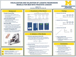
1.  The most common malignancy diagnosed in men
 The second leading cause of death from cancer among
men in United States
 More than 230,000 new cases to be diagnosed and more
than 30,000 deaths estimated for 2013
 A special treatment for men with newly-diagnosed
prostate cancer at early stage
 Relieve patients from unnecessary pain
 May lead to metathesis if not properly identified
 The most sensitive method of detecting bone metastasis
 Crucial for deciding the optimal course of treatment
 Accessible, noninvasive, has low radiation dose, and has
an ability to evaluate the entire skeletal system; however
it is time-consuming (3-4 hours) and costly ($600-$1,000)
 Most sensitive scan for detecting lymph node metastasis
 Accessible, minimally invasive and painless; however it is
risky with more radiation and costly ($300-$1,500)
To visualize the
prediction results generated from risk models
To evaluate the calibration
and discrimination performance for predictive risk models
I.
Jianyu Liu
University of Michigan, Ann Arbor, MI
To determine the probability of a positive AS or BS or CT as a function of
several covariates consisting of patient age, prostate-specific antigen (PSA),
clinical tumor stage, Gleason score, and percentage of biopsy positive cores.
For k explanatory variables and n individuals, the LRM is:
log
𝑝𝑖
1 − 𝑝𝑖
= 𝛼 +
𝑗=1
𝑘
𝛽𝑗 𝑥𝑖𝑗
where pi is the probability that the patient i has a positive AS or BS or CT
 Widely used for internal validation of LRM (1000 random samples drawn)
 Expected optimism: the average difference between the performance of
models developed in each sample and their original performance
 ROC area: quantifies the ability of the prediction models to discriminate
between patients with and without AS or BS or CT
 R2: quantifies the explained variation on the log-likelihood scale
 Calibration slope: slope of the linear predictor of the LRMs
Well-calibrated models have a slope of 1, while models providing
extreme predictions have slope less than 1
 ROC area > 0.8: the model has great discrimination
 R2 > 30%: the model is explanatory
 Calibration Slope > 0.9 (close to 1): the model has
great calibration
 By embodying developed LRMs in an iOS
application, the predicted probability of having
cancer metathesis can be estimated
 Visualization of models can help clinicians make
better screening and treatment decisions
 LRMs for AS, BS, and CT are stable to use with
great discrimination and calibration
 Save treatment costs and extend patient lifespan
II.
ROC area 0.888 0.873 0.855
R2 43.5% 38.6% 32.1%
Calibration slope 1 0.88 0.938
Training set
(n =643)
Internally
validated
Validation
set (n =507)
ROC area 0.844 0.822 0.811
R2 34.0% 27.6% 29.4%
Calibration slope 1 0.83 0.962
Internally
validated
Training set
(n =416)
Validation
set (n =664)
Optimisimb
ROC area 0.022 ± 0.031 0.031 ± 0.013 0.015 ±0.021 0.014 ± 0.028
R2
6.44% ± 7.90% 4.82% ± 2.03% 4.90% ± 6.0% 10.34% ± 2.21%
Shrinkage factor 0.83 ± 0.22 0.80 ± 0.23 0.88 ± 0.14 0.92 ± 0.16
Optimism-corrected performancec
ROC area 0.822 0.802 ± 0.014 0.873 0.863 ± 0.031
R2 27.60% 25.7% ± 4.7% 38.60% 30.1% ± 4.5%
Calibration slope 0.83 0.80 ± 0.23 0.88 0.92 ± 0.16
a
Expected performance was based on training datasets, and observed performance was based on validation sets. Means and empirical standard errors are
shown. 1000 bootstrap samples were used for calculation of the means and SETraining , and SEValidation.
b
The expected optimism was calculated as the difference between bootstrap performance and test performance. The observed optimism was calculated as
the difference between apparent performance in training sets and observed performance in the validation sets.
c
The optimism-corrected performance was defined as apparent performance - optimism. The observed optimism-corrected performance is equal to the
oberserved performance in validation sets.
Bone Scan CT Scan
Expected, mean ±
SETraining (n= 416)
Observed, mean ±
SEValidation (n= 664)
Expected, mean ±
SETraining (n= 643)
Observed, mean ±
SEValidation (n=507)