1. 1 | John Cronin SULI- Summer 2015 Introduction, Materials & Methods
Producing Realistic Future Trajectories for Irrigated Agriculture Under Saline Conditions
Using the Crop Production Optimization Model APSIDE.
John Cronin
U.S. Department of Energy Office of Science, Science Undergraduate Laboratory Internship
(SULI)
University of California, Merced
Lawrence Berkeley National Laboratory
Berkeley, California
August 7th, 2015
Prepared in partial fulfillment of the requirements of the U.S. Department of Energy Office of
Science, Science Undergraduate Laboratory Internship (SULI) under the direction of Nigel
Quinn in the Earth Sciences Division at Lawrence Berkeley National Laboratory.

2. 2 | John Cronin SULI- Summer 2015 Introduction, Materials & Methods
Abstract
APSIDE is a model that simulates water quality and salinity, as well as agricultural
production, in the west side of the San Joaquin Valley. This model is useful in understanding
water in the San Joaquin Valley in response to changes in California’s long term water
allocation. The motivation for developing this model is to have an agricultural production model
that takes groundwater into account. The importance of this model has become even more
apparent considering the current state of water in California. Moreover, a changing climate will
likely have an effect on California’s water in the future. This will certainly increase the
importance and utilization of APSIDE and other models like it. The initial APSIDE model could
run for five water districts in the San Joaquin Valley, and the input data was over 10 years old.
The model was updated using recent data from the USGS. The model was also expanded to run
for an additional 14 water districts in the San Joaquin Valley. In its current state, these expanded
water districts run with estimated data. In the future, more accurate data will be added so the
model can have accurate output for the expanded water districts. Updating the model caused an
increase in simulated water salinities within APSIDE. Values like deep percolation and lateral
flow in APSIDE were compared to a USGS model called CVHM. This comparison showed that,
on average, APSIDE simulates lower values of deep percolation and upflux than CVHM. On
average, CVHM’s deep percolation values were 26 % higher in Panoche WD, 12.9 % higher in
Broadview WD, 45.3 % higher in San Luis WD, and 51.3 % higher in Pacheco. When predicting
future hydrology and crop yields, APSIDE simulates changing irrigation techniques. This is
reflected in irrigation efficiencies in the model. CVHM is a flow model, and does not take this
into account. This comparison helped to better understand the hydrological portion of APSIDE.

3. 3 | John Cronin SULI- Summer 2015 Introduction, Materials & Methods
I. Introduction
A changing climate will likely have an effect on the world’s agricultural production. This
is because a changing climate can have an effect on water availability as well as temperature,
which in turn can have an effect on plant yields (Parry et al. 2004). The San Joaquin Valley is
one of the world’s largest producers of agricultural goods (Schoups et al. 2005). Understanding
water availability and water quality, in particular, is critical to understanding agricultural
production in the San Joaquin Valley.
The San Joaquin Valley typically receives a limited amount of rainfall. Water is essential
for plant growth, so changing water availability can have a direct effect on yields. Water also
plays a key role in soil salinity. All water used for agriculture, even if it is high quality, contains
some salt (van Hoorn, 2006). Applied irrigation water is subject to the processes of direct
evaporation from the soil surface and transpiration from the crop. Pure water is evaporated,
leaving behind the salts in irrigation water. Over time, these salts can accumulate in the soil and
groundwater and can affect agricultural yields. A large problem in the San Joaquin Valley is that
salts are imported with irrigation water. Excess water can leach out salts in soil profile (van
Hoorn, 2006). The western San Joaquin Valley is particularly affected by salinity due to limited
water (Schoups et al. 2005). Since the semi-arid climate of the San Joaquin Valley receives little
rainfall, there is not a lot of excess water to leach these soils of salts. Typically, excess irrigation
water is applied to leach salts (Abrol et al. 1988). This cost of this can add up quickly, and there
is not always a large enough water supply for this to be possible. In order to understand
agricultural production in the San Joaquin Valley, it is important to understand water quality and
availability.

4. 4 | John Cronin SULI- Summer 2015 Introduction, Materials & Methods
A state-of-the-art model known as the Central Valley Hydrologic Model, or CVHM, has
been developed by the USGS. The model simulates the effects of hydraulic conductivity,
irrigation, streamflow losses, wells, and other parameters on groundwater flow (Faunt et al.
2009). This state of the art model is used by many to understand groundwater in the Central
Valley.
A crop production and hydrosalinity model has been developed called the Agricultural
Production Salinity Irrigation Drainage Economics model, or APSIDE. This model was
developed to simulate agricultural production as a result of long-term changing water allocations
as well as impacts on groundwater and salinity (Quinn, 2004). This model is currently able to
predict crop production as a function of a number of state variables including water supply,
groundwater pumping, irrigation water quality, as well as root zone and groundwater salinity.
The objective function within APSIDE is a profit maximization algorithm, which maximizes
income from crop production. This includes costs associated with production, including
irrigation and groundwater pumping expenses. APSIDE is unique in its ability to simulate the
effects of salinity on production. APSIDE attempts to maximize profit by minimizing crop yield
losses as a result of soil and water salinity (Quinn, 2004).
The current APSIDE model simulates the agricultural production within a five water
district area in the San Joaquin River Basin, on the western side of the San Joaquin Valley. The
model was created around fifteen years ago, and calibrated with data from that time. Data from
the Central Valley Hydrological Model is being used to update and improve the current APSIDE
model. The updated APSIDE model uses output from the CVHM and simulates groundwater
quality and salinity to simulate agricultural production in this five district area. In addition to
updating APSIDE, the model may also be expanded to more than the current five water district

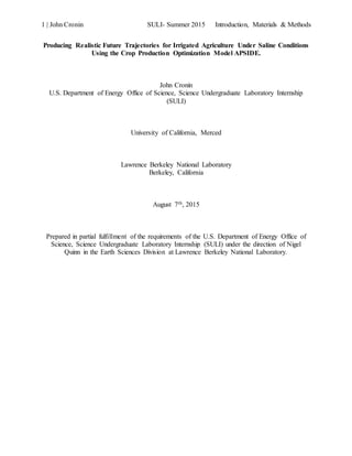
5. 5 | John Cronin SULI- Summer 2015 Introduction, Materials & Methods
area. Updating APSIDE using output from CVHM will make the model more useful for planning
studies..
II. Methods
The APSIDE model was developed using the Generalized Algebraic Modeling System,
or GAMS. The model simulates productivity and yield in response to changes in water quality,
water supply, as well as groundwater and root zone salinity. It also predicts the quality and flows
of future agricultural drainage.
The current APSIDE model simulates crop production and hydrosalinity in five water
districts. These water districts are: San Luis Water District, Panoche Water District, Pacheco
Water District, Broadview Water District, and Westlands Water District (Figure 1). These water
districts are all found on the western edge of the San Joaquin River Basin.
These water districts are represented
by defined geospatial locations. Polygons
corresponding to the water districts were
created using ArcGIS. Data from the CVHM
is also located geospatially. A GIS was used,
to overlay the data from CVHM on to the
water district’s footprint. ArcMap was used
as the geospatial database for this task. The
GIS program allows us to append USGS data
to each of the water districts. Once all of the
necessary state variables are determined, they
can used as input data for APSIDE.
Figure 1. Area of interest in grey and
corresponding waterdistricts.

6. 6 | John Cronin SULI- Summer 2015 Introduction, Materials & Methods
Creating polygons
Within APSIDE, each water district is treated as a single unit. The data that comes from
CVHM corresponds to a mesh composed of 1 mile square polygons. This mesh has 98 columns
and 441 rows that cover the entire San Joaquin Valley. This information had to be aggregated so
each water district could be treated as a singular unit. This is done by creating the water district
polygons by using the smaller existing polygons within CVHM’s mesh. All of the data from
CVHM directly corresponds to the water districts of interest.
The centroid of each polygon was determined using arcMap, and the centroids of
adjacent polygons were connected. Groundwater flow between polygons can be assigned to these
connections. Ideally, flow between adjacent polygons occurs orthogonally to the water district
boundary creating a large cross section through which the water flows.
Adding geospatial data
The data from CVHM that we are interested in using corresponds to the 1 𝑚𝑖2
mesh, and
it is formatted like the mesh. The output is in table format with 98 columns and 441 rows, and
each value corresponds to a 1 mile square cell in the grid. This data was added to arcMap using a
‘grid to column’ tool. This tool converts the data from CVHM to a form that can be applied to
arcMap.
Using GIS we can then subset the data we are working with to include only that which applies to
our water district area.
Data that was updated in APSIDE includes include land usages, base values for inter-
district groundwater flow, district sizes, depth to Corcoran clay layer, and thickness of Corcoran
clay layer. The significance of these updates is discussed in the results section of this paper.
APSIDE Model

7. 7 | John Cronin SULI- Summer 2015 Introduction, Materials & Methods
APSIDE performs water and salt balance for each individual district, so all of the state
variables that correspond to the water districts must also be singular. CVHM includes
information about all of the 1 mile square polygons that make up the entire water district. An
average of all the values that APSIDE uses can be taken over the entire area of each water
district polygon; APSIDE treats the entire district as a subarea. APSIDE will use these average
values and assign a singular value to each water district. APSIDE makes use of CONOPT2,
which is a non-linear solver, to determine optimal monthly solutions to the objective function
(GAMS Development Corporation, 1998).
The effectiveness of updating APSIDE can be determined by comparing the model to its
pre-updated state. With more recent and detailed input, the model should simulate agricultural
production and salinity more accurately. That being said, APSIDE may require some additional
refinement as newer data is added to the model.
CVHM Comparison & Zonebudget
Data from APSIDE was compared to a state-of-the-art groundwater model, called the
Central Valley Hydrologic Model, or CVHM. CVHM is able to show the movement of water
from user-defined spatial areas through the use of a post-processing tool called Zonebudget. The
movement of water between zones was simulated using Zonebudget. Zonebudget is a post-
processing tool that converts the cell to cell flow in CVHM to text for analysis. There is an ‘i-
bound’ array that is used to define the zones that are of interest to you. It is 98 columns, 441
rows, and 13 layers deep. Each APSIDE water district was given a unique zone identifier. In
addition to this, each water district was divided into three vertical layers. For example, the upper
layer in Broadview Water District was assigned the value 971. The second layer was assigned
972, and the third layer was assigned 973. This allowed flows to be looked at in the upper, mid,

8. 8 | John Cronin SULI- Summer 2015 Introduction, Materials & Methods
Figure 2. Initial water districtsin
Tan, expanded water districtsin
color.
and lower portions of the soil profile. The Zonebudget output was compared to the hydrologic
output in APSIDE. Values that were compared include deep percolation, upflux, and lateral flow.
Initial Expansion
The initial APSIDE model corresponded to a five water district area. APSIDE was
expanded to contain a total of twenty-two water districts
(Figure 2). This was done using ArcGIS to create polygons
corresponding to the additional water districts.
Water districts hydrology can be simulated within the
APSIDE model. The values in the expanded model are
estimated values to ensure that the model can run for these
districts. In the future, more refined input data will be added to
these regions to accurately simulate agricultural production,
water salinity, and water quality in these water districts.
III. Results & Discussion
Hydrologic output data from APSIDE was compared to CVHM output from the post-
processing tool called Zonebudget. Deep percolation and upflux values in acre-feet per year were
simulated using both models and compared. The results of the preliminary analysis show that the
deep percolation and upflux values in APSIDE were lower, on average, than the results of
CVHM’s simulation (Appendix A). If it is deemed necessary to increase or decrease the deep
percolation, upflux, or lateral flow values in APSIDE, it can be done fairly easily. By changing
hydraulic conductivity values, these values can be easily increased or decreased in APSIDE.
Typically, the amount of water allowed to percolate through the upper region of the soil profile is

9. 9 | John Cronin SULI- Summer 2015 Introduction, Materials & Methods
around 10% of the total water delivery (Grismer 1990). It is important to make sure these values
are as accurate as possible within the model. Deep percolation drives the leaching of salts from
the root zone. Upflux can bring salt into the root zone from the water table. APSIDE’s simulated
values over a 25 year period were compared to the CVHM output. APSIDE’s values for upflux
were 17.2% lower in Panoche, 22.6% lower in San Luis, and 49.2% lower in Pacheco. For deep
percolation, APSIDE’s values were 26% lower in Panoche, 12.9% lower in Broadview, 45.3%
lower in San Luis, and 51.3% lower in Pacheco.
The deep percolation values in APSIDE and CVHM were compared to reported data in
Panoche and Pacheco Water Districts. Pacheco Water District reported deep percolation values
of 1770 acre-feet on 4080 acres of irrigated land (Pacheco Water District 2010). This
corresponds to a deep percolation of 0.43 acre-feet per acre. This aligns fairly closely to
APSIDE’s predicted values ranging between 0.41 and 0.44 acre-feet per acre (Westcot et al.
1994).
APSIDE was expanded from five districts to a total of twenty-two water districts. These
districts all fall within the San Joaquin Valley. The input data for these districts will need to be
updated in the future. The input data for these districts can be added fairly easily. Most of the
data that is pertinent to APSIDE has already been published by the USGS, and is contained
within the input files for the CVHM.
A number of initial conditions for APSIDE were updated using data from the USGS.
Each water district has unique values for a number of hydrological parameters. The parameters
that were updated are: base values for inter-district flow, current crop choices, depth to Corcoran
clay layer, thickness of Corcoran clay layer, and the total area of each district. Doing this
resulted in changes in APSIDE’s simulation of groundwater salinity. The average total dissolved

10. 10 | John Cronin SULI- Summer 2015 Introduction, Materials & Methods
salts, TDS, for unconfined aquifers are shown (Appendix B). In the unconfined aquifer, salinity
simulations increased by 1.3% in Broadview, 1.2% in Panoche, 3.1% in Pacheco, and 1.4% in
San Luis. The updated APSIDE model simulated an increase in groundwater salinity in the
unconfined aquifer; for all districts the change was less than 0.4%. This result is expected
because of the Corcoran Clay layer preventing large movement of water and salt into the
confined aquifer. More saline groundwater can result in yield losses; the increase in salinity can
result in yield losses. There is a possibility that the groundwater table elevates upwards and into
the root zone. If groundwater is saline, then this can result in yield losses. Another possibility is
yield losses due to pumped saline groundwater. The increase in salinity of groundwater can
reduce crop yields if the salinity rises above the crops’ yield reduction threshold (Maas 1977).
Another parameter that was updated in APSIDE was the land usages. Land usage refers
to the acres within each district that are designated for a certain crop in a given year. For
example, in 2013 Broadview water district had 5120 acres of cotton and 640 acres of field crops.
By updating this data, APSIDE takes into account crop choices that are being made in the water
district. This has an effect on water needed for irrigation, costs of labor, possible yield losses.
Crops that are salt tolerant will be less affected by soil salinity and water salinity; these crops
will experience little to no yield decline when compared to salt effected crops. Updating the land
usages for APSIDE caused a change in root zone concentration of salts when compared to the
initial (earlier) model. There were also changes to the deep percolation concentration, tile
drainage salinity concentrations, and predicted crop acreages in APSIDE (Appendix C). The
average changes in deep percolation salinities for Pacheco Water District were less than 0.35%.
Deep Percolation Concentrations increased by 5% in Broadview, 1.4% in Panoche, and
decreased by 7.9% in San Luis. The average change in Root Zone salinities increased by 3.3% in

11. 11 | John Cronin SULI- Summer 2015 Introduction, Materials & Methods
Broadview, 1.6% in Panoche, and decreased by 7.5% in San Luis. Tile drainage salinities
increased by .5% in Panoche and decreased by 2.8% in San Luis. There is no tile drainage in
Broadview, and thus there was no change reflected in the updated model’s salinity simulations
for this value.
IV. Conclusions
Moving forward, APSIDE will be used to better understand water salinity and water
quality within salt-affected agricultural areas within the San Joaquin Basin. By updating the
input data for APSIDE, the model more accurately reflects current conditions as well as past
trends. This should improve the models simulations in the future.
If trends in California water follow the current trajectory, water deliveries will become
even more restricted. APSIDE can help to maximize agricultural production and increase
efficiencies in water shortages. APSIDE is a predictive model; the model can be used to predict
salinities and water deliveries. In turn, APSIDE chooses crops that maximize profits for the land
owner.
When the expansion of this model is completed, APSIDE will run for a total of twenty-
two water districts. This will increase the utility of the model, and hopefully contribute to a better
understanding of hydrology and agriculture in the San Joaquin Valley.
It will be important, if possible, to continually update the APSIDE model to ensure that it
reflects the most up to date and accurate input data. In addition, it will be useful to compare the
updated APSIDE’s results to actual observations to ensure that the model continues to simulate
in an accurate manner.

12. 12 | John Cronin SULI- Summer 2015 Introduction, Materials & Methods
V. Acknowledgements
This work was supported in part by the U.S. Department of Energy, Office of Science, Office of
Workforce Development for Teachers and Scientists (WDTS) under the Science Undergraduate
Laboratory Internship (SULI) program. I would like to thank my mentor, Nigel Quinn, for his
guidance and knowledge during this project. I would also like to thank the entire HEADS team
for their continued support of this work.

13. 13 | John Cronin SULI- Summer 2015 Introduction, Materials & Methods
Literature Cited
[1] Abrol, I. P., Jai Singh Pal Yadav, and F. I. Massoud. "6. WATER QUALITY AND CROP
PRODUCTION." Salt-affected Soils and Their Management. Rome: Food and
Agriculture Organization of the United Nations, 1988. N. pag. Print.
[2] Faunt, C.C., Hanson, R.T., Belitz, K., Schmid, W., Predmore, S.P., Rewis, D.L.,
McPherson, K.R., 2009. Numerical model of the hydrologic landscape and
Groundwater flow in California's Central Valley (Chapter C). In: Faunt, C.C. (Ed.),
Groundwater Availability of the Central Valley Aquifer, California: U.S.
Geological Survey Professional Paper 1776, pp. 121-212
.[3] GAMS Development Corporation, Brooks, A., Kendrick, D., Meerhaus, A., Raman, R.,
1998. GAMS: A User’s Guide. GAMS Development Corporation, Washington, DC.
[4] Grismer ME. Leaching fraction, soil salinity, and drainage efficiency. Calif Agr. 1990.
44(6):24 -7.
[5] Harbaugh, Arlen W. "MODFLOW: USGS Three-dimensional Finite-difference Ground-
water Model." MODFLOW: USGS Three-dimensional Finite-difference Groundwater
Model. N.p., n.d. Web. 25 July 2015.
[6] Maas, E. V., and Hoffman. "Testing Crops for Salinity Tolerance." U.S. Salinity Laboratory,
USDA-ARS (1977): n. pag. Print.Pacheco Water District. Water Management Plan. pp.27-
29.
[7] Parry, M.l, C. Rosenzweig, A. Iglesias, M. Livermore, and G. Fischer. "Effects of Climate
Change on Global Food Production under SRES Emissions and Socio-economic
Scenarios." Global Environmental Change 14.1 (2004): 53-67.

14. 14 | John Cronin SULI- Summer 2015 Introduction, Materials & Methods
[8] Quinn, N.w.t., L.d. Brekke, N.L. Miller, T. Heinzer, H. Hidalgo, and J.a. Dracup. "Model
Integration for Assessing Future Hydroclimate Impacts on Water Resources, Agricultural
Production and Environmental Quality in the San Joaquin Basin, California."
Environmental Modelling & Software 19.3 (2004): 305-16.
[9] Schoups, G., J. W. Hopmans, C. A. Young, J. A. Vrugt, W. W. Wallender, K. K. Tanji, and
S.
Panday. "." Proceedings of the National Academy of Sciences 102.43 (2005): 15352-
5356.
[10] Van Hoorn, J.W. and van Alphen, J.G. (2006), Salinity control. In: H.P. Ritzema (Ed.),
Drainage Principles and Applications, p. 533, Publication 16, International Institute for
Land Reclamation and Improvement (ILRI), Wageningen, The Netherlands.ISBN 90-
70754-33-9
[11] Westcot, Dennis, Ross Steensen, Stuart Styles, and James Ayars. "Grassland Basin
Irrigation and Drainage Study." Irrigation Training and Research Center (1994): n. pag.
Web. 04 July 2015.

15. 15 | John Cronin SULI- Summer 2015 Introduction, Materials & Methods
Appendix A
Note:
Within the discretization file in MODFLOW (“DIS”) the units of the model can be
established. By setting the values for ITMUNI to 5 and LENUNI to 1 the model will run in terms
of years and English units. For this analysis, the units were converted manually to ft/year from
meters cubed per day. The units must be consistent throughout the input files for CVHM
(MODFLOW MANUAL - Harbaugh 2005).
0
0.1
0.2
0.3
0.4
0.5
0.6
0.7
Feet
Panoche Upflux, Acre-Feet per Acre
APSIDE
CVHM Zonebudget
0
0.2
0.4
0.6
0.8
1
Feet
Panoche Deep Percolation, Acre-Feet per Acre
CVHM Zonebudget
APSIDE
The predicted APSIDEupfluxes and the CVHM outputsare shown above.The same analysiswas made for
all water districts. This is an example forPanoche.
The predicted deep percolation values in APSIDE were compared to the deep percolation output in CVHM.
Above is an example showing the deep percolation in Panoche water district.

16. 16 | John Cronin SULI- Summer 2015 Introduction, Materials & Methods
17.2%
22.6%
49.2%
0
10
20
30
40
50
60
PAN SLW PCH
Average Percent Difference, Upflux
APSIDE & CVHM
% Difference
26 %
12.9 %
45.3 %
51.3 %
0
10
20
30
40
50
60
PAN BVW SLW PCH
Average Percent Difference, Deep Percolation
APSIDE & CVHM
% Difference
The average differences over a 25 year period between APSIDE and CVHM for the waterdistricts.
Broadview was left out due to lossof water deliveries, making upflux valuesincorrect. Upflux Values in
CVHM are larger than APSIDE.
The average differences over a 25 year period between APSIDE and CVHM for each water district
are shown above. The deep percolation values in CVHM are larger than in APSIDE.

17. 17 | John Cronin SULI- Summer 2015 Introduction, Materials & Methods
APPENDIX B
1490
1492
1494
1496
1498
1500
1502
2015 2016 2017 2018 2019 2020 2021 2022 2023 2024 2025
mg/L
Pacheco TDS - Confined Aquifer
Updated
Initial
1475
1480
1485
1490
1495
1500
1505
1510
2015 2016 2017 2018 2019 2020 2021 2022 2023 2024 2025
mg/L
Panoche TDS - Unconfined Aquifer
Updated
Initial
1.3 % 1.2%
3.1%
1.4%
0
0.5
1
1.5
2
2.5
3
3.5
BVW PAN PCH SLW
% Change, Unconfined AquiferTDS
% Change
TDS in the confined aquifer increased by less than 0.4% in all districts. This is expected
because the Corcoran clay layer prevents large movement of salts into the confined aquifer.
Changesin Panoche’s unconfined aquifer are shown above. Panoche’sunconfined aquifersalinity
decreased by 1.2%.
The changes in APSIDE’s predicted salinities are shown above.The salinity in the unconfined aquifer
increased in all districts.

18. 18 | John Cronin SULI- Summer 2015 Introduction, Materials & Methods
Appendix C
The updated model simulates a lower concentration of salt in the root zone at Broadview Water
District when compared to the initial model.
In San Luis Water District, the updated model shows an increase in the salinity of deep
percolation water when compared to the initial model.
3700
3800
3900
4000
4100
4200
4300
4400
4500
4600
2015 2016 2017 2018 2019 2020 2021 2022 2023 2024
Broadview Root Zone Concentration
Updated
Initial
4200
4400
4600
4800
5000
5200
2015 2016 2017 2018 2019 2020 2021 2022 2023 2024
PPM
San Luis Deep PercolationSalinity
Updated
Initial
6400
6450
6500
6550
6600
6650
2015 2016 2017 2018 2019 2020 2021 2022 2023 2024
PPM
Panoche Tile Drainage Concentration, PPM
Updated
Initial
The tile drainage concentration in Panoche Water District stays nearly the same for the first
six years of the simulation, then the updated model simulates lower salinity concentration for
the next four years.

19. 19 | John Cronin SULI- Summer 2015 Introduction, Materials & Methods
-10
-8
-6
-4
-2
0
2
4
6
ROOT ZONE
CONCENTRATION
DEEP PERC CONCENTRATION TILE DRAIN TDS
% Change Salinities for Each District
Broadview
Panoche
San Luis
The changesin rootzoneconcentration,deep percolation concentration,and tiledrainageTDSin
the updated and initialmodels.Broadview and Panocheshowed increases,whileSan Luisshowed
decreasesin salinities.