
Recomendados
Recomendados
Mais conteúdo relacionado
Mais procurados
Mais procurados (18)
Semelhante a On the methodology of isew, gpi... (neumayer, 2000)
Semelhante a On the methodology of isew, gpi... (neumayer, 2000) (20)
Mais de Introsust
Mais de Introsust (20)
Último
Último (20)
On the methodology of isew, gpi... (neumayer, 2000)
- 1. Ecological Economics 34 (2000) 347–361 ANALYSIS On the methodology of ISEW, GPI and related measures: some constructive suggestions and some doubt on the ‘threshold’ hypothesis Eric Neumayer London School of Economics and Political Science, Houghton Street, London WC2A 2AE, United Kingdom Received 14 October 1999; received in revised form 26 January 2000; accepted 27 January 2000 Abstract Existing country studies of the Index of Sustainable Economic Welfare (ISEW), the Genuine Progress Indicator (GPI) and related measures, while sharing the same basic methodological approach, differ with respect to the valuation of important items. This paper provides a critical, but constructive, discussion of the various methods used for the valuation of non-renewable resource depletion and long-term environmental damage, and for the weighting of consumption expenditures for income inequalities. Several recommendations are given on how to improve the methodology for future updates of existing studies or for the construction of new measures. Sensitivity analysis shows that if these recommendations are followed for the valuation of resource depletion and long-term environmental damage, then the so-called ‘threshold’ hypothesis, which seems to have gained empirical support from all studies undertaken so far, fails to materialise. This suggests that, as far as factors related to the environment are concerned, the widening gap between ISEW and GPI on the one hand and gross national product (GNP) on the other, might be an artefact of highly contestable methodological assumptions. © 2000 Elsevier Science B.V. All rights reserved. Keywords: Index; Welfare; Sustainability; Resources; Environmental damage; Inequality www.elsevier.com/locate/ecolecon 1. Introduction Following the pioneering work by Daly et al. (1989) and Cobb and Cobb (1994) for the US, the construction of an Index of Sustainable Economic Welfare (ISEW) has become quite popular with studies undertaken for an increasing number of countries. An ISEW has, for example, been con- structed for Austria (Stockhammer et al., 1997), Chile (Castan˜eda, 1999), Germany (Diefenbacher, 1994), Italy (Guenno and Tiezzi, 1998), the Netherlands (Rosenberg, Rosenberg et al., 1995), Scotland (Moffatt and Wilson, 1994), SwedenE-mail address: e.neumayer@lse.ac.uk (E. Neumayer). 0921-8009/00/$ - see front matter © 2000 Elsevier Science B.V. All rights reserved. PII: S0921-8009(00)00192-0
- 2. E. Neumayer / Ecological Economics 34 (2000) 347–361348 (Jackson and Stymne, 1996) and the UK (Jackson et al., 1997). Sometimes these studies come, with only slightly changed methodology, under the name of Genuine Progress Indicator (GPI), as, for example, in Australia (Hamilton, 1999) and the US (Redefining Progress, 1999). For Australia, there also exists a related measure, which comes under the name of sustainable net benefit index (SNBI) (Lawn and Sanders, 1999). Computation of an ISEW/GPI usually starts from personal consumption expenditures. These expenditures are weighted with an index of in- come inequality. Then, certain welfare-relevant contributions are added, such as the services of household labour and the services of streets and highways, whereas certain welfare-relevant losses are subtracted, such as so-called ‘defensive expen- ditures’, costs of environmental pollution, costs of depletion of non-renewable resources and long- term environmental damage costs. The resulting index is regarded as a more accurate indicator of sustainable economic welfare than a country’s gross national product (GNP), which, according to proponents of ISEW/GPI, even if not origi- nally invented for such a purpose, is used by policy makers and in everyday language as a yardstick for economic welfare.1 The methodology used for ISEW/GPI studies has been criticised by some authors, including the present one (see Nordhaus, 1992; the contribu- tions in Cobb and Cobb, 1994; Atkinson, 1995; Neumayer, 1999a,b). However, whereas Neu- mayer (1999b), for example, provides a general conceptual critique, this paper’s objective is more confined and more concrete. It aspires to put forward some constructive suggestions on the methodology used for ISEW, GPI and related measures, and to shed some doubt on the so- called ‘threshold hypothesis’. More specifically, it focuses on three items: the valuation of the deple- tion of non-renewable resources (Section 2), the valuation of long-term environmental damage (Section 3) and the adjustment of consumption expenditures for income inequality (Section 4). These items exert a significant influence on most ISEW/GPI and related measures. In evaluating the results of their work, propo- nents of ISEW/GPI have put great emphasis on a clearly discernible trend of the ISEW/GPI in al- most all studies undertaken so far: starting from around the 1970s or early 1980s, depending on the country, the ISEW/GPI no longer rises very much or even falls, whereas GNP continues to rise. As an explanation for this widening gap between ISEW/GPI and GNP, Max-Neef (1995, p. 117) has put forward the so-called ‘threshold hypothe- sis’: ‘for every society there seems to be a period in which economic growth (as conventionally measured) brings about an improvement in the quality of life, but only up to a point — the threshold point — beyond which, if there is more economic growth, quality of life may begin to deteriorate’. This ‘threshold hypothesis’ is referred to in almost every recent ISEW/GPI study and Max-Neef (1995, p. 117) himself regarded the evidence from these studies ‘a fine illustration of the Threshold Hypothesis’. Anielski (1999, p. 3) suggests that the hypothesis confirms ‘what many Americans and Canadians feel and are experienc- ing — the economy and stock exchanges may be soaring but average citizens sense the steady ero- sion of their economic quality of life’. This paper argues that proponents of ISEW/ GPI consider their results too easily as evidence for the ‘threshold hypothesis’. It suggests that, as far as depletion of non-renewable resources and long-term environmental damage contribute to the widening gap between ISEW/GPI and GNP, this gap might be the artefact of highly con- testable methodological assumptions. Sensitivity analysis is employed to demonstrate that these items no longer give rise to a threshold if the assumption of a cost escalation factor in the valuation of non-renewable resource depletion and the assumption of cumulative long-term envi- ronmental damage is abandoned. 1 Some studies refer to gross domestic product (GDP) in- stead of GNP. The difference between GNP and GDP is that GDP includes output produced by foreigners within the na- tional boundaries and excludes output produced by nationals abroad. As the difference between GNP and GDP does not matter here, the following paragraphs usually only refer to GNP, except when a study explicitly refers to GDP.
- 3. E. Neumayer / Ecological Economics 34 (2000) 347–361 349 2. Depletion of non-renewable resources As concerns the depletion of natural resources, the method used by various studies differs on three major aspects: first, either replacement costs or resource rents are used to compute the deduc- tion item; second, either national consumption or national extraction is the reference for valuation; and, third, if the resource rent method is used, then either total resource rents are deducted or the so-called El Serafy method is used for calcu- lating resource user costs, which are then de- ducted. 2.1. Replacement costs or resource rents? Let us start with the first and most fundamental difference. The ambiguity between either using the resource rent method or the replacement cost method stems back to the original US ISEW. Whereas Daly et al., (1989) and Cobb and Cobb (1994) in their original ISEW computations de- ducted the total value of mine extraction, the revised ISEW in Cobb and Cobb (1994) switched to the replacement cost method: for non-renew- able energy extraction each barrel of oil equiva- lent was valued at a replacement cost which was assumed to escalate by 3% per annum between 1950 and 1990 and was anchored around an assumed cost of $75 in 1988. The Austrian, Ger- man and Italian ISEW followed Daly et al., (1989) in deducting the total value of mine pro- duction. The Australian SNBI study also applied the resource rent method, but computed user costs according to the El Serafy method. The Chilean, Dutch, Scottish, Swedish and UK ISEW and the Australian and US GPI, on the other hand, followed the replacement cost method of the revised ISEW in Cobb and Cobb (1994) to- gether with the 3% escalation factor. There is a clear rationale for using the resource rent method: because non-renewable resources are irreversibly lost in the process of use, non-renew- able resource extraction represents the (partial) liquidation of an existing capital stock. Rental income that accrues from resource extraction is, therefore non-sustainable into the future and should either fully (total resource rents) or partly (user costs according to El Serafy method) be deducted. The resource rent method is inspired by the idea of sustainable income and aims to sepa- rate the sustainable from the non-sustainable in- come parts. The rationale for using the replacement cost method, on the other hand, is completely different. It stems from the idea that non-renewable resource use, which cannot be pro- longed forever and is therefore, not sustainable into the indefinite future, would have to be re- placed by renewable resources. The replacement cost method suffers from two major problems, however: first, the underlying assumption is that non-renewable resource use has to be fully replaced by renewable resources in the present; second, the escalation factor assumes that replacement costs increase over time. As con- cerns the first problem, there is no convincing rationale for why non-renewable resources would have to be fully replaced by renewable resources in the present when there are still available re- serves that would last for many decades. For example, the static reserves to extraction ratio, which gives the time of how long proven reserves would last at current extraction levels, was 41 years for oil, 63 years for natural gas and 218 years for coal at the end of 1998 (British Petroleum, 1999).2 If non-renewable resources are cheaper than renewable resources, as Cobb and Cobb (1994) assume and is certainly correct for energy resources, then a rational resource extrac- tor would be foolish not to use up the remaining non-renewable resources first, before switching to renewable resources later on. For the same rea- son, it seems odd to deduct replacement costs for the totality of resource use in the present year. The relatively high replacement cost of 75 US$ in 1988, which has been taken over by other studies as well, only makes sense if total current non-re- newable resource use would need to be replaced 2 On the one hand, the static reserves to extraction ratio overestimates available resource reserves as extraction is likely to increase in the future. On the other hand, it underestimates available resource reserves as new reserves become available. For example, while oil extraction has increased from 58 mil- lion barrels per day in 1973 to about 72 million barrels per day in 1998, proven oil reserves have not only failed to decrease, but have even increased from 630 thousand million barrels to 1050 thousand million barrels (British Petroleum, 1999).
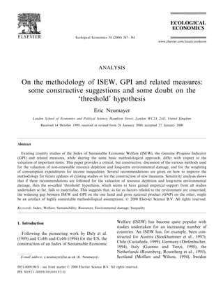
- 4. E. Neumayer / Ecological Economics 34 (2000) 347–361350 with renewable resources in the present. Again, this bears the question why a rational resource extractor should switch to extremely expensive renewable replacement resources, when much cheaper non-renewable resources are still avail- able. Why not wait with switching until some point in the future, when switching becomes nec- essary and is likely to be much cheaper as the technology for the extraction and use of renew- able resources will have improved? Related to this last point is the second problem, the 3% escalation factor, which has also rather uncritically been taken over by other studies. As a rationale for this assumption of constantly in- creasing replacement costs, Cobb and Cobb (1994, p. 267) refer to the costs per foot of oil drilling which they report to have increased by about 6% per annum during the period of high oil prices in the 1970s, which triggered the explo- ration and drilling of more difficult to exploit oil fields. They reason that ‘when the limits of a resource are being reached, the cost of extracting the next unit is more costly than the previous unit’ and that ‘this principle presumably applies also to renewable fuels, though not as dramatically as to oil and gas’, which is why the escalation factor is assumed to be 3 instead of 6%. Especially with respect to renewable energy resources, such rea- soning might be erroneous, however. The most likely candidate for replacing non-renewable fuels is renewable solar energy. But the solar energy influx exceeds current world energy demand by at least one order of magnitude (Norgaard, 1986), so that the limits of this resource are unlikely to be reached. Also, costs for solar energy use are cur- rently high because the technology is still in the early stages of development, but costs will fall over time as technology improves (Lenssen and Flavin, 1996). Instead of assuming replacement costs to escalate by 3% per year, it might therefore be more appropriate to assume that replacement costs are falling over time. The replacement cost method with the 3% esca- lation factor contributes to the ‘threshold hypoth- esis’. The method computes the deduction term as RC(t)=R(t)· 75 $ ·1.03(t−1988) where R is resource use and t is the year of computation. This deduction term will rise over time if R does not fall by more than 3% per annum. What is more, the deduction term will rise at a rate faster than GNP if the growth rate of GNP is smaller than 3% plus the growth rate of resource use: RC · RC GNP · GNP if GNP · GNP B0.03+ R · R , where a dot above a variable represents its partial derivative with respect to time. If resource use does not fall significantly and GNP grows at a rate of less than 3%, which is not uncommon, then the replacement method together with the 3% escalation factor, ceteris paribus, causes an increasing gap between GNP and the ISEW/GPI, thus contributing to the ‘threshold hypothesis’. Exactly this has happened in the existing studies, as Fig. 1 shows, which presents the indexed trend of GNP/GDP together with the indexed trend for resource depletion with the 3% escalation factor for a selection of four country studies: the Dutch, Swedish, US and UK ISEW.3 As can be seen, the indexed trend for resource depletion with the 3% escalation factor is growing at a faster rate than the indexed trend of GNP/GDP, thus causing a widening gap over time. Ceteris paribus, this widening gap will translate into a widening gap between a country’s ISEW and its GNP/GDP and create evidence for the ‘threshold hypothesis’. The replacement cost method together with the 3% escalation factor has a substantial influence on the ISEW or GPI. The item depletion of natural resources represents, for example, approximately 37% of all deduction items in the US ISEW in 1990, 31% in the UK ISEW in 1996, 21% in the Swedish ISEW in 1992 and 36% in the Dutch ISEW in 1992. If instead replacement costs are not assumed to escalate by 3% per annum, but, for the sake of argument, are assumed to remain constant, then the item ‘depletion of non-renewable resources’ no longer gives rise to a ‘threshold hypothesis’. 3 Because the threshold hypothesis refers to a period during the 1970s or early 1980s, for ease of exposition 1970 is the start year in the figure.
- 5. E. Neumayer / Ecological Economics 34 (2000) 347–361 351 Fig. 1. (a) The Netherlands ISEW. (b) Sweden ISEW. (c) United Kingdom ISEW. (d) United States ISEW.
- 6. E. Neumayer / Ecological Economics 34 (2000) 347–361352 Fig. 1. (Continued)
- 7. E. Neumayer / Ecological Economics 34 (2000) 347–361 353 See Fig. 1 again, which also shows the indexed trend for resource depletion without the escala- tion factor. In the US and the UK indexed GNP/ GDP is now rising faster than resource depletion due to decreasing non-renewable resource inten- sity of GNP/GDP, thus creating the opposite of a threshold effect.4 In the Swedish and Dutch case, both trends have a similar shape over time, so that resource depletion does not contribute to a widening gap between ISEW and GDP. 2.2. Resource production or resource consumption? In the last section, it has not been made clear whether resource use refers to the extraction or consumption of resources. The reason is that some studies differ on this respect. On the one hand, all studies using the resource rent method value the extraction of resources. This is correct as the resource rent method attempts to determine the sustainable parts of an income stream derived from resource extraction. Only rents from re- source extraction, not from consumption, enter the national income accounts. Therefore, to de- duct the value of consumption instead would mean to deduct something that has never been added in the first place. On the other hand, the studies using the re- placement cost method are not consistent in their reference point. Whereas the revised US ISEW in Cobb and Cobb (1994) and the US GPI estimate the cost for replacing national extraction, the Australian GPI and the Chilean, Dutch, Scottish, Swedish and UK ISEW estimate the cost for replacing national consumption of non-renewable resources. Methodologically correct is the valua- tion of consumption, not extraction. This is be- cause the rationale behind the method is to replace non-renewable resource use. Where these resources come from, whether they are imported or domestically extracted, simply does not matter. The idea behind the replacement cost method is not to cancel out non-sustainable income streams, as it is with the resource rent method. Instead, the idea is to estimate the costs of replacing all non- renewable resources in use for production. 2.3. Total resource rents or user costs according to the El Serafy method? Finally, those studies that use the resource rent method are not unanimous on whether to deduct total resource rents or merely the user costs com- puted according to the El Serafy method. Total resource rents are deducted in the original US, Austrian, German and Italian ISEW, whereas the Australian SNBI study uses the El Serafy method. The difference matters as user costs are in general only a fraction of total resource rents (see the appendix to this paper). In my view, the El Serafy method is to be preferred. This is because, given substitutability between natural capital in the form of non-renew- able resources and other forms of capital, such as manufactured or human capital, the finite income stream from a non-renewable resource stock can be transformed into a lower infinite stream of income from other forms of capital (Hartwick 1996). What the El Serafy method does is to compute the difference between these two income streams and to deduct the resulting so-called user costs of non-renewable resource extraction. De- ducting total resource rents instead implies that one cannot sustain an infinite stream of income from a finite non-renewable resource via investing the resource rents into other forms of capital (see also Neumayer, 2000). 3. Long-term environmental damage As concerns the valuation of long-term environ- mental damage, or the costs of climate change as this item is sometimes called, the fundamental question is whether this value should accumulate over time or not. All but the Australian GPI study have opted for accumulation. It is the objec- tive of this section to show that accumulation is incorrect. Most studies follow the approach taken by Daly et al. (1989) and Cobb and Cobb (1994) in valuing each barrel of oil equivalent of annual 4 The same holds true for the US GPI, which is not shown here for reasons of space limitations.
- 8. E. Neumayer / Ecological Economics 34 (2000) 347–361354 nonrenewable energy resource consumption at $0.50 in 1972 dollars. This value is deducted from the ISEW in this year, but also in all following years. Similarly, in any given year not only the value for current resource consumption is de- ducted, but the values from all past years as well. Cobb and Cobb (1994, p. 74) provide as justifica- tion for this accumulation approach that they ‘imagined that a tax or rent of $0.50 per barrel- equivalent had been levied on all non-renewable energy consumed during that period and set aside to accumulate in a non-interest-bearing account (...). That account might be thought of as a fund available to compensate future generations for the long-term damage caused by the use of fossil fuels and atomic energy.’ Jackson et al. (1997, p. 23) realise in their computation of the UK ISEW that ‘the major problem with this approach (...) is the arbitrary way in which a charge is calculated’. Instead they purport to value each tonne of greenhouse gas emissions with its marginal social cost, which they correctly define as reflecting ‘the total (dis- counted) value of all the future damage arising from that tonne of emissions’. Strangely, however, they follow Cobb and Cobb (1994) in letting this damage accumulate over time. Stockhammer et al. (1997) similarly compute marginal social dam- age costs for the Austrian ISEW — and let the estimated damage accumulate over time. Accumulation is theoretically incorrect (Atkin- son, 1995; Neumayer, 1999a). This is easiest to see with the UK ISEW study. In valuing each tonne of emissions with its marginal social cost, the total future damage of this tonne of emissions is al- ready valued. To let this value accumulate over time is self-contradictory and therefore simply wrong as it leads to multiple counting of the total future damage. Jackson et al. (1997) value each tonne of carbon with a marginal social cost of £11.4 in 1990 prices. With accumulation, the present value damage caused by one tonne of carbon is simply infinite without discounting or £11.4/r with discounting, where r is the discount rate. With a discount rate of, say, 5% per annum, the present value damage per tonne of carbon is £228. This present value damage per tonne of carbon of £228 is nothing else but the marginal social cost per tonne of carbon, which contradicts Jackson et al.’s earlier assumption of marginal social cost of £11.4 (Jackson et al., 1997). That accumulation is incorrect is not as straightforward to show with the Cobb and Cobb (1994) approach, as they do not base their valua- tion on marginal social costs. Instead, as men- tioned, they justify valuing long-term environ- mental damage from fossil fuel consumption by $0.50 per barrel of oil equivalent with the idea that this would represent the money to be set aside in order to compensate future generations for long-term environmental damage. As before, however, accumulation leads to multiple counting here as well. This is because with accumulation money for the damage caused by each unit of emissions is set aside not only in the year of emission, but for each subsequent year as well. Again, the present value of damage caused, but this time per barrel of oil equivalent, is equal to $0.50/r, which equals $10 at a discount rate of 5% per annum. With a carbon content of 0.13 tonnes per barrel of oil (Poterba, 1991), this translates into a present value damage per tonne of carbon of about $75, which is much smaller than the £228 of the UK ISEW. Note that I do not claim here that a marginal social cost per tonne of carbon of $75 (US ISEW) or £228 (UK ISEW) would be unjustifiable. It is true that $75 is close to the upper end of damage cost estimates as reported in IPCC (1996, pp. 179–224) and £228 is way beyond the most pes- simistic upper estimation end. But, given uncer- tainty and ignorance about the exact consequences of global warming, such high esti- mates are not absurd per se. However, if propo- nents of ISEW think that the marginal social cost per tonne of carbon emitted is so high, then they should make their assumption explicit and they should not use methodologically incorrect accumulation. The accumulation of long-term environmental damage costs exerts a substantial influence on the ISEW or GPI. This item represents, for example, approximately 33% of all deduction items in the US ISEW in 1990, 23% in the UK ISEW in 1996, 30% in the Swedish ISEW in 1992 and 12% in the Dutch ISEW in 1992. Accumulation of long-term
- 9. E. Neumayer / Ecological Economics 34 (2000) 347–361 355 environmental damage costs also contributes to the ‘threshold hypothesis’. Fig. 2 presents the indexed trend of GNP/GDP together with the indexed trend of accumulated long-term environ- mental damage and non-accumulated long-term environmental damage. As can be seen, the in- dexed trend for accumulated long-term environ- mental damage is growing much faster than the indexed trend of GNP/GDP, thus causing a widening gap over time. As with the item resource depletion when replacement costs are assumed to escalate at 3% per annum, this widening gap will ceteris paribus, translate into a widening gap be- tween a country’s ISEW and its GNP/GDP, thus contributing to the ‘threshold hypothesis’. If instead long-term environmental damage is not accumulated, then it no longer gives rise to a ‘threshold hypothesis’. See Fig. 2 again. In the US and the UK indexed GNP/GDP is now rising faster than long-term environmental damage due to decreasing emission intensity of GNP/GDP, thus creating the opposite of a threshold effect.5 In the Swedish and Dutch case, both trends have a similar shape over time, so that long-term envi- ronmental damage does not contribute to a widening gap between ISEW and GDP.6 One might think that even if long-term environ- mental damage is not accumulated over time, a threshold effect might still arise if marginal social costs per tonne of emitted carbon are assumed to increase over time. To let marginal social costs increase over time is correct as the marginal social cost per tonne of emitted carbon is a positive function of the accumulated stock of carbon still resident in the atmosphere. In other words, the higher the historically accumulated carbon con- centration in the atmosphere, the higher the social damage caused by each additional unit of emitted carbon. Jackson et al. (1997, p. 24) actually follow this approach in assuming ‘firstly that the mar- ginal social cost in 1990 is equal to £11.4 per tonne [of carbon, E.N.], and secondly that the marginal social cost in any year is proportional to the cumulative carbon emissions from the year 1900 up to that point in time [emphasis added].’ It can be seen, however, from Fig. 2 for the UK ISEW that a threshold effect does not arise even if marginal social cost is increasing over time, as long as the annual damage itself is not accumu- lated over time. Whether a threshold effect can arise under differing, but still plausible assump- tions about the rate of increase of marginal social cost deserves some further attention and cannot be ruled out at this stage with confidence. But at least for the UK ISEW, the only study so far using rising marginal social costs, the threshold effect fails to materialise. 4. Adjustment for inequality As concerns adjusting consumption expendi- tures for income inequalities, studies differ quite substantially on the method chosen, which is partly to be explained by international differences in the availability of relevant data. It would be beyond the scope of this paper to provide a full discussion here. Instead I will concentrate on a fundamental difference between the approach taken in the UK ISEW and in the rest of the studies. 4.1. Atkinson index or other indices? Whereas Jackson et al. (1997) use an index, which allows the choice of a parameter represent- ing society’s aversion to inequality, all other stud- ies use an index, mostly the Gini coefficient, which does not offer such a choice. Jackson et al. use the so-called Atkinson index (Atkinson 1970), which is defined as: Atkinson index=1−exp %(Yi/Y)1/(1−m) fi n1/(1−m) where Yi denotes the income of all individuals in the ith income group (n groups altogether), fi denotes the proportion of the population with incomes in the ith range; and Y denotes the mean income. The extreme boundary cases are m=0, 5 The same result holds true for the Austrian, German and Italian ISEW, which is not shown here for reasons of space limitations. 6 The same result holds true for the Chilean ISEW (not shown here).
- 10. E. Neumayer / Ecological Economics 34 (2000) 347–361356 Fig. 2. (a) The Netherlands ISEW. (b) Sweden ISEW. (c) United Kingdom ISEW. (d) United States ISEW.
- 11. E. Neumayer / Ecological Economics 34 (2000) 347–361 357 Fig. 2. (Continued)
- 12. E. Neumayer / Ecological Economics 34 (2000) 347–361358 which implies no aversion to inequality whatso- ever, and m=
- 13. , which implies extreme aversion to income inequality in only taking account of transfers to the very lowest income group. The great advantage of this approach is that in choosing m, the researcher makes explicit his or her implicit assumption on society’s aversion to income inequality. Alternatively, the researcher can try to estimate o from revealed preference studies of consumer behaviour. Pearce and Ulph (1995), for example, provide an estimate of m for the UK from a survey of the empirical literature with a lower bound of 0.7, an upper bound of 1.5 and a best estimate of 0.8. If instead, for example, the Gini coefficient is used, then usually 1 year is set as the base year for the index. In the US GPI, for example, which uses the Gini coefficient, 1968 is set as 100, because ‘it represented the lowest Gini coefficient over the 1950–1998 period, thus the least income inequal- ity. All other years are then compared to this benchmark’ and an index is created (Redefining Progress, 1999). The inequality adjusted consump- tion expenditures are reached via dividing unad- justed expenditures by this index and multiplying with 100. This approach is very ad hoc and the researcher’s underlying assumptions about soci- ety’s aversion to income inequality are not expli- cated. With the Atkinson index, on the other hand, the researcher is forced to explicate his or her implicit assumptions regarding society’s aver- sion to income inequality The researcher can even attempt to minimise the influence of his or her own value judgements in trying to estimate soci- ety’s revealed preferences. 4.2. Index of welfare or sustainable income? In using an index of inequality to adjust con- sumption expenditures, great care needs to be applied to adequately interpret the resulting ISEW/GPI. More generally, as soon as indexing is applied to one of its items, interpretation must follow either of two lines: First, the ISEW/GPI can be interpreted as an index as well. If so, then only changes in the index over time can meaning- fully be interpreted. For example, one can say that the ISEW/GPI rose or fell in a certain year by x percent. The absolute level of the ISEW/ GPI, on the other hand, bears no meaning and should not be referred to then. Second, if the ISEW/GPI is interpreted in absolute terms rather than as an index, then a statement is needed on what the base year of indexing part of its compo- nents has been. This is because the absolute level of ISEW/GPI crucially depends on choosing a base year for indexing as the reference point. Thus, the US GPI per capita in 1997, for example, needs to be stated as follows: 6521 in constant chained 1992 dollars with base year 1968 for income inequality indexing. Related to this point, the ISEW/GPI needs to be interpreted as a measure of welfare, not as sustainable or Hicksian income. Amongst other things, this is because, due to the indexing, the resulting ISEW/GPI cannot be interpreted as the income that society can safely consume and be as well off at the end of the year as at the beginning. Daly et al. (1989, p. 84) were clearly aware of this crucial point. Lately, however, this distinction seems to have become blurred. England (1998, p. 265), for example, in praising ISEW suggests that it ‘is directly comparable to gross domestic product’. However, the absolute level of ISEW/ GPI cannot be directly compared to the absolute level of GNP as the absolute level of ISEW/GPI is weighed by an index for income inequality, whereas GNP is not. Meaningful comparison is confined to the trend of ISEW/GPI over time compared to the trend of GNP. 5. Conclusion From the analysis above follow several recom- mendations for researchers who intend to update existing or create new studies of ISEW, GPI or related measures. First, if one uses the resource rent method for the valuation of non-renewable resources, then the reference point should be na- tional extraction of non-renewable resource deple- tion, not consumption, and one should consider estimating user costs according to the El Serafy method instead of deducting total resource rents. Second, if one uses the replacement cost method, then the reference point should be national con-
- 14. E. Neumayer / Ecological Economics 34 (2000) 347–361 359 sumption of non-renewable resources, not extrac- tion, and some thought should be given to whether the totality of non-renewable resources needs to be replaced in the present. More impor- tantly, future researchers should seriously con- sider abandoning the 3% cost escalation factor. Third, long-term environmental damage should not be accumulated, as doing so leads to multiple counting. Fourth, future researchers should con- sider using the Atkinson index if they want to adjust consumption expenditures for income in- equality, as this index demands explication of the implicit assumption about society’s aversion to inequality. Fifth, with indexing applied to any of its items, the resulting ISEW/GPI cannot be di- rectly compared to GNP in absolute terms. While it is tempting to do so, no such comparison is meaningfully possible. Only trends over time can be compared. The analysis in this paper has also shed some light on the robustness of the ‘threshold hypothe- sis’. It has been shown that if no escalation factor is applied to valuing the depletion of non-renew- able resources, and if long-term environmental damage is not accumulated, then none of these items contributes any longer to a widening gap between ISEW/GPI and GNP. The other environ- mentally related items in a typical ISEW/GPI, such as costs of water, air and noise pollution, generally do not contribute to such a gap either, as they do not grow faster than GNP (for reasons of space they could not be dealt with here in more detail). One can therefore conclude from the anal- ysis above that variables related to the environ- ment do not provide evidence for the ‘threshold hypothesis’. They only do so if a widening gap between ISEW/GPI and GNP is artificially cre- ated via the introduction of the 3% cost escalation factor and the accumulation of long-term environ- mental damage. This does not provide sufficient evidence against the ‘threshold hypothesis’ in general, as other factors covered by ISEW/GPI might still create a widening, but smaller, gap between ISEW/GPI and GNP/GDP. Related research has shown that, in general, the ‘threshold hypothesis’ is not simply an artefact of the cost escalation factor in non-renewable resource depletion and of the accumulation of long-term environmental damage in all studies (Saito, 1999). To analyse the more general robustness of the ‘threshold hypoth- esis’, one needs to examine each study in much more detail. Such a task would be beyond the scope of this paper and is the subject of ongoing research. What this paper has tried to show, however, is that the threshold, if existent, is not due to factors related to the environment. Acknowledgements I would like to thank Mako Saito for valuable research assistance. I would also like to thank Giles Atkinson and two referees, Saleh El Serafy and Phil Lawn, for helpful comments. I am grate- ful to Clive Hamilton and Mark Anielski for an enormously productive exchange of ideas and ar- guments — we tend to agree that we disagree. All errors are mine. Financial assistance from the European Commission’s Marie Curie Research Scheme (DGXII) is gratefully acknowledged. Appendix A. Derivation of user costs according to the El Serafy method The formula for computing user costs accord- ing to the El Serafy method is derived from the following reasoning (El Serafy, 1989): receipts from non-renewable resource extraction should not fully count as ‘sustainable income’ because resource extraction leads to a lowering of the resource stock and thus brings with it an element of depreciation of the capital that the resource stock represents. While the receipts from the re- source stock will end at some finite time, ‘sustain- able income’ by definition must last forever. Hence, ‘sustainable income’ is that part of re- source rents which if received infinitely would have a present value just equal to the present value of the finite stream of resource rents over the lifetime of the resource. Let P be the resource price, AC average extrac- tion cost, R the amount of resource extracted, r the discount rate and n the number of remaining years of the resource stock if extraction was the
- 15. E. Neumayer / Ecological Economics 34 (2000) 347–361360 same in the future as in the base year, i.e. n is the static reserves to extraction ratio. Then the present value of total resource rents RR (P− AC)·R is equal to: % n i=0 RR (1+r)i = RR 1− 1 (1+r)n+1 n 1− 1 1+r (1) The present value of an infinite stream of ‘sustain- able income’ SI is %
- 16. i=0 SI (1+r)i = SI(1+r) r = SI 1− 1 1+r (2) Setting Eq. (1) and Eq. (2) equal and rearranging expresses SI as a fraction of RR: SI=RR 1− 1 (1+r)n+1 n The user costs, representing the depreciation of the resource stock, would thus be (RR−SI)=RR 1 (1+r)n+1 n =(P−AC) · R 1 (1+r)n+1 n If r0 and n0, then user costs are only a fraction of total resource rents (P−AC)·R. The higher r is, the lower are, ceteris paribus, user costs. This is because a smaller share of resource rents has to be invested in an alternative form of capital in order to provide a sustainable alterna- tive income stream if the rate of return on this alternative investment is higher. Similarly, the higher n is, the lower are user costs. This is because, for given resource extraction, a smaller share of the total resource stock is used up. References Anielski, M., 1999. Misplaced concreteness: Measuring gen- uine progress and the nature of money, paper presented at the Canadian Society for Ecological Economics Confer- ence, 28 August 1999. Regina, Saskatchewan. Atkinson, A.B., 1970. On the measurement of inequality. J. Econom. Theory 2, 244–263. Atkinson, G., 1995. Measuring Sustainable Economic Welfare: A Critique of the UK ISEW, Working paper GEC 95-08. Centre for Social and Economic Research on the Global Environment, Norwich and London. British Petroleum, 1999. BP Statistical Review of World En- ergy. British Petroleum, London. Castan˜eda, B.E., 1999. An index of sustainable economic welfare (ISEW) for Chile. Ecolog. Econom. 28, 231–244. Cobb, C.W., Cobb, J.B., 1994. The Green National Product: a Proposed Index of Sustainable Economic Welfare. Univer- sity Press of America, Lanham. Daly, H., Cobb, H.E., Cobb, J.B., 1989. For the Common Good. Beacon Press, Boston. Diefenbacher, H., 1994. The index of sustainable economic welfare: a case study of the Federal Republic of Germany. In: Cobb, C.W., Cobb, J.B. (Eds.), The Green National Product: A Proposed Index of Sustainable Economic Wel- fare. University Press of America, Lanham, pp. 215–245. El Serafy, S., 1989. The proper calculation of income from depletable natural resources. In: Ahmad, Y.J., Serafy, S.E., Lutz, E. (Eds.), Environmental Accounting for Sustainable Development: A UNDP-World Bank Symposium. The World Bank, Washington D.C, pp. 10–18. England, R.W., 1998. Should we pursue measurement of the natural capital stock? Ecolog. Econom. 27, 257–266. Guenno, G., Tiezzi, S., 1998. An index of sustainable eco- nomic welfare for Italy, Working paper 5/98. Fondazione Eni Enrico Mattei, Milano. Hamilton, C., 1999. The genuine progress indicator: methodo- logical developments and results from Australia. Ecolog. Econom. 30, 13–28. Hartwick, J.M., 1996. Sustainability and constant consump- tion paths in open economies with exhaustible resources. Rev. Int. Econom. 3, 275–283. IPCC, 1996. Climate Change 1995 — Economic and Social Dimensions of Climate Change. Cambridge University Press, Cambridge. Jackson, T., Stymne, S., 1996. Sustainable Economic Welfare in Sweden: A Pilot Index 1950–1992. Stockholm Environ- ment Institute, Stockholm. Jackson, T., Laing, F., MacGillivray, A., et al., 1997. An Index of Sustainable Economic Welfare for the UK 1950– 1996. University of Surrey Centre for Environmental Strat- egy, Guildford. Lawn, P.A., Sanders, R.D., 1999. Has Australia surpassed its optimal macroeconomic scale? finding out with the aid of ‘benefit’ and ‘cost’ accounts and a sustainable net benefit index. Ecolog. Econom. 28, 213–229. Lenssen, N., Flavin, C., 1996. Sustainable energy for tomor- row’s world — the case for an optimistic view of the future. Energy Policy 24, 769–781. Max-Neef, M., 1995. Economic growth and quality of life: a threshold hypothesis. Ecolog. Econom. 15, 115–118. Moffatt, I., Wilson, M.C., 1994. An index of sustainable economic welfare for Scotland, 1980–1991. Int. J. Sustain. Dev. World Ecol. 1, 264–291.
- 17. E. Neumayer / Ecological Economics 34 (2000) 347–361 361 Neumayer, E., 1999a. Weak Versus Strong Sustainability: Exploring the Limits of Two Opposing Paradigms. Edward Elgar, Cheltenham. Neumayer, E., 1999b. The ISEW: not an index of sustainable economic welfare. Social Indic. Res. 48, 77–101. Neumayer, E., 2000. Resource accounting in measures of unsustainability: Challenging the World Bank’s conclu- sions, Environ. Resource Econ. 15, 257–278. Nordhaus, W.D., 1992. Is growth sustainable?, Reflections on the concept of sustainable economic growth, paper pre- pared for the International Economic Association Confer- ence, October 1992. Varenna. Norgaard, R.B., 1986. Thermodynamic and economic con- cepts as related to resource-use policies: synthesis. Land Econom. 62, 325–327. Pearce, D., Ulph, D., 1995. A Social Discount Rate for the United Kingdom, Working Paper GEC 95-01. Centre for Social and Economic Research on the Global Environ- ment, UK. Poterba, J.M., 1991. Tax policy to combat global warming: on designing a carbon tax. In: Dornbusch, R., Poterba, J.M. (Eds.), Global Warming: Economic Policy Responses. MIT Press, Cambridge (Mass), pp. 33–98. Redefining Progress, 1999. The 1998 U.S. Genuine Progress Indicator: Methodology Handbook, Redefining Progress, San Francisco. Rosenberg, D., Oegema, P., Bovy, M., 1995. ISEW for the Netherlands: Preliminary Results and Some Proposals for Further Research. IMSA, Amsterdam. Saito, M., 1999. An Index of Sustainable Economic Welfare — Can it Be Evidence for the ‘Threshold hypothesis’. London School of Economics, London. Stockhammer, E., Hochreiter, H., Obermayr, B., Steiner, K., 1997. The index of sustainable economic welfare (ISEW) as an alternative to GDP in measuring economic welfare: the results of the Austrian (revised) ISEW calculation 1955– 1992. Ecolog. Econom. 21, 19–34. .