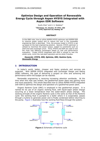
1. COMMERCIAL-IN-CONFIDENCE HTFS RS 1230
Optimize Design and Operation of Renewable
Energy Cycle through Aspen HYSYS Integrated with
Aspen EDR Software
Guofu Chen1 and V. V. Wadekar2
1TAS Energy, Inc. Houston, TX 77021, USA
2HTFS, AspenTech Ltd, Reading, UK
ABSTRACT
In this R&D note, how to utilize ASPEN HYSYS optimizer and ASPEN EDR
to improve power output and to reduce the cost in the renewable
engineering field is described. First, the process model in HYSYS is set
up based on the best engineering practice. Second, HYSYS optimizer is
utilized to maximize the power output, subject to constraints such as
shell and tube exchanger pinch. Third, HYSYS and EDR are used to size
the most cost effective exchangers based on cost and performance
evaluation. Finally HYSYS integrated with EDR is utilized to rate the
whole cycle, mimic the real plant operation and do what-if studies.
Keywords: HYSYS, EDR, Optimize, ORC, Rankine Cycle,
- 1 -
Renewable Energy
1 INTRODUCTION
In today’s world, better, cheaper and faster products and services are
expected. With ASPEN HYSYS integrated with Exchanger Design and Rating
(EDR) software, the goal of delivering a project on time and achieving the
performance within the budget can be reached.
Renewable engineering is receiving increasing attention worldwide. At the
time when this note was written, the geothermal power plant was gaining more
and more popularity. This article describes how to utilize ASPEN HYSYS integrated
with EDR to optimize the design and operation of a geothermal power plant.
Organic Rankine Cycle (ORC) is employed in the geothermal project. It is
named for its use of an organic working fluid, with liquid-vapor phase change
occurring at a lower temperature than the water-steam phase change. The
working principle of the organic Rankine cycle is the same as that of the Rankine
cycle: the working fluid is pumped to a boiler where it is evaporated, passes
through a turbine to generate power and is finally condensed before returning to
the pump. Figure 1 illustrates how the working fluid flows through the system.
Figure 1 Schematic of Rankine cycle

2. COMMERCIAL-IN-CONFIDENCE HTFS RS 1230
Figure 1 is useful as a schematic diagram but it hides the complexity of a
geothermal power plant. In such a plant there is complex interaction among
many operating equipment. Furthermore, optimization of the entire power plant
is a challenging task which cannot be carried out without commercial software
tools for process simulation and detailed exchanger modelling.
In order to illustrate one out of many optimization challenges posed by a
geothermal power plant, Figure 2 is prepared. This shows that, if we focus on the
Expander, generating the power, and the downstream air-cooled condenser
determining the condensation pressure, there is a trade-off between the energy
generated by the Expander and energy consumed by the cooling fan of the air-cooled
condenser. The top blue curve shows that as the condensing pressure
increases the power output of the expander falls linearly. The power consumed
by the air-cooler fan also falls with increasing condensing pressure. The red
curve shows this non-linear variation. The difference between these two curves,
after the relatively constant pump power consumption is deducted, is the net
power generation as shown by the green curve which goes through a maximum,
i.e. the optimum condensing pressure.
Figure 2 Net power output vs. condensing pressure
Figure 2 was produced for a specific working fluid and operating conditions as
described later. Figure 2 will be revisited in Section 4.1 for a more detailed
discussion.
Through the use of HYSYS and EDR software the complex interactions of
various equipment and optimisation challenges, such as that illustrated in Figure
2, can be addressed. The whole step-wise sequence of developing the process
model, of increasing degree of granularity, from simple conceptual design to
optimization of the plant operation is described in the following sections.
2 SETTING UP HYSYS PROCESS MODEL
In this application, R134a is chosen as the working fluid, with RefProp physical
- 2 -
property package selected in HYSYS.
As described in Figure 1, there are four major components in the cycle. Figure
3 shows how the cycle looks after the model is built in HYSYS.
In this project, for the evaporator the hot stream flow rate of 794.9 m3/h
(3500 GPM) is known and so also the inlet and outlet temperature of 140.6 °C

3. COMMERCIAL-IN-CONFIDENCE HTFS RS 1230
(285 °F) and 60 °C (140 °F). The duty of the evaporator can be calculated as
6.0×107 kcal/h (2.4×108 Btu/hr).
For the Air-Cooled Condensers (ACC), the ambient air dry bulb temperature of
10 °C (50 °F) is known. Considering 13.9 °C (25 °F) temperature difference
between the inlet air and outlet working fluid, ACCOut temperature can be
calculated as 23.9 °C (75 °F). Since the outlet of the ACC is at the saturated
liquid condition, ACCOut pressure can be calculated as 6.436 bara (93.35 psia).
The pump discharge pressure is a key process parameter to be optimized. At
this time 44.82 bara (650 psia) pump discharge pressure and 81% pump
efficiency are assumed, and PumpOut temperature is calculated as 26.46 °C
(79.63 °F). After the throttling valve downstream of the pump, EvaporatorIn
enthalpy is calculated as -2144 kcal/kg (-3856 Btu/lb).
The working fluid outlet temperature EvaporatorOut is very critical to the
process as well. The EvaporatorOut temperature of 115.6 °C (240 °F) is
assumed as initial value, and the corresponding enthalpy of EvaporatorOut is
calculated as -2093 kcal/kg (-3764.56 Btu/lb). From the heat balance, the
working fluid mass flow can be calculated as 1.177×106 kg/h (2.594×106 lb/hr).
After the expansion valve upstream of the expander, all the process conditions
of flow, pressure and temperature are known. The expander efficiency of 87% is
assumed. The expander discharge pressure can be calculated from the
condensing pressure of ACCOut, assuming a certain pressure drop in ACC and the
pipe. This corresponds to an ExpanderOut pressure of 6.781 bara (98.35 psia).
Then the expander can be solved for the shaft power of 1.03×104 kW (1.38×104
HP).
Through the isenthalpic flashing, all the process conditions of ACCIn are
known. The ACC duty can be calculated as 5.205×107 kcal/h (2.064×108 Btu/hr)
since ACCOut is at the saturated liquid condition.
After HYSYS is converged, through the HYSYS spread sheet, the Expander
generator electricity output and the power consumption of the pump are
calculated. Thus the net output is calculated. Please note at this time, the ACC
fan motor power consumption is not calculated yet.
Figure 3 Cycle schematic in HYSYS
3 HYSYS OPTIMIZER TO MAXIMIZE POWER OUTPUT
As mentioned in the previous section, PumpOut pressure and EvaporatorOut
temperature are key process parameters to be optimized. The HYSYS optimizer
is now utilized to find out the optimum combination of the pressure and
temperature.
- 3 -

4. COMMERCIAL-IN-CONFIDENCE HTFS RS 1230
The optimizer is set up to maximize the net output, by adjusting the PumpOut
pressure and EvaporatorOut temperature, subject to the constraint that the
evaporator pinch should be larger than 5.56 °C (10 °F).
The “Original Data Model” is chosen in the Optimizer Configuration tab and
“Box” Scheme is selected in the Parameters tab. The EvaporatorOut temperature
is limited between 93.33 °C (200 °F) and 135 °C (275 °F). Because higher
pressure will lead to more expensive exchangers, the PumpOut pressure is limited
to be lower than 50.33 bara (730 psia), see “High Bound” column in Figure 4.
Referring to Figure 5, the net output is imported to cell B2 and the minimal
approach is imported to cell B3 of OptimizerSpreadSheet.
By pushing the “Start” button, HYSYS optimizer starts to find the solution that
maximizes the net power output, while respecting the constraints of exchanger
pinch and the range of temperature and pressure.
After HYSYS finishes the optimization, the optimum pressure is 50.33 bara
(730 psia) and the optimum temperature is 122.67 °C (252.8 °F). At such
conditions, the net power output is maximized at 8635 kW (1.158×104 HP).
Figure 4 Optimizer variables set up
Figure 5 Optimizer goal and constraints set up
- 4 -

5. COMMERCIAL-IN-CONFIDENCE HTFS RS 1230
4 RIGOROUS EXCHANGER MODELING
Now the optimum conditions are found from the thermodynamic point of view
Then the question becomes, are exchangers sized at optimum conditions as well?
The next step is to find cost effective designs for the air-cooled condensers and
the evaporator. To describe this, Figure 6, which shows the cycle in further
details, is used.
4.1 Optimize the Number of Air-Cooled Condenser Bays
To make Air-Cooled Condensers (ACC) cost effective and reliable, TAS Energy
has made a standard bay size. For smaller project, only one or two bays are
used, while for larger projects 30 bays or more can be deployed.
To have a fair comparison regarding the evaporator size, in this calculation,
the UA of the evaporator is specified, rather than the EvaporatorOut temperature.
Aspen Air-Cooled Exchanger integrated with HYSYS is used to perform rigorous
simulation of the ACC. To avoid the pump cavitations in case the ACC does not
fully condense the working fluid, a dummy cooler is added to make sure that the
outlet fluid is saturated liquid before entering the pump, see Figure 6 for more
details.
Figure 6 ORC cycle simulation with exchanger geometries in HYSYS
ACCIn pressure is specified and an “adjust” is used to adjust the ACC air flow
rate so that the dummy exchanger duty is 0. Since cost and performance will be
evaluated, the ACC fan power consumption is calculated through HYSYS
spreadsheet and it’s deducted to get net power output.
ACC condensing pressure can be higher if smaller air flow rate is used, which
saves power on the ACC fans, but reduces the expander output (gross power) as
well. Or the ACC condensing pressure can be lower to generate more expander
output, but it demands more air flow that increases ACC fan power consumption.
Thus an optimum condensing pressure is desired.
In this project, 30 bays ACC is used as a starting point. Again through HYSYS
optimizer, the maximum net power output by changing ACCIn pressure is
targeted. Please notice at any fixed condensing pressure, the “Adjust” adjusts
the air flow to make sure the outlet of the ACC is at the saturated liquid
condition.
After the HYSYS optimizer is finished, the optimum condensing pressure is
calculated as 6.567 bara (95.25 psia), which gives the maximum net output at
8209 kW (11008 HP). This optimization can be done through “Case Studies”
function in HYSYS as well. Figure 2 in Section 1 illustrates how condensing
pressure relates to the generator output (gross output), fans power consumption
and the net output.
- 5 -

6. COMMERCIAL-IN-CONFIDENCE HTFS RS 1230
Next the condensing pressure for 24, 27, 33, 36 and 39 bays is optimized
individually, based on the same approach. The results are summarized in Table 1
and 24 bays is considered as base case for comparison purpose.
From Table 1, we can see the incremental cost per kW is 2207, 2651, 3289,
3790, and 4166 $/kW. Depending on how the desired power output is evaluated,
different number of ACC bays may be chosen. Based on the prevalent
geothermal industry criterion of the incremental cost of about 3000 $/kW, 30
bays for the air-cooled condensers is finally selected. See Figure 8 for details.
Figure 7 Air-cooled exchanger in HYSYS
Figure 8 Incremental cost vs. number of ACC bays
- 6 -
Geothermal
industry criterion

7. COMMERCIAL-IN-CONFIDENCE HTFS RS 1230
Table 1 Optimization of air‐cooled condensers ACC
No of Bays 24 27 30 33 36 39
ACC cost $ 3,600,000 4,050,000 4,500,000 4,950,000 5,400,000 5,850,000
Condensing
Temperature °C 25.53 24.68 23.65 22.81 21.91 20.95
Condensing
Pressure bara 6.964 6.757 6.567 6.378 6.188 5.998
Air Flow kg/h 17,463,485 18,127,638 18,847,410 20,048,988 21,296,251 23,188,787
Net Output kW 7,835 8,039 8,209 8,346 8,464 8,572
Incremental
cost $/kW ‐ 2,207 2,651 3,289 3,790 4,166
4.2 Optimize the Size of the Evaporator
Now we optimize the size of the evaporator. Please note that from process
stand point, CoolWaterOut temperature is fixed. If EDR rating integrated with
HYSYS is used, the CoolWaterOut temperature will be a variable, which will not
give us fair comparison. To achieve this, UA of the evaporator is fixed in the
HYSYS calculation, while using the “Shell and Tube Exchanger Utility” to size the
exchanger dimension and estimate the cost. The “Shell and Tube Exchanger
Utility” is able to size the exchanger with given process conditions, while not
affecting HYSYS calculation.
In a separate study, not discussed here, two exchangers in parallel and two in
series with 18.29 m (60 ft) long tubes were found to give the most cost effective
solution within these constraints. The number of tubes and the shell diameter
can be varied. Within these constraints, the shell and tube exchanger utility gives
us the geometry and the cost.
Then the UA of the evaporator is multiplied by 0.9, 1.1 1.3 and 1.5
respectively. Following the same steps as before, exchanger size, cost and net
output for each scenario are summarized in Table 2.
From Table 2, incremental cost to generate one more kW is 864, 1337, 2438,
and 3612 $ respectively. Based on about 3000 $/kW as the economic criterion,
the exchanger with 1118 mm (44 inch) shell diameter is finally chosen, see
Figure 9.
Figure 9 Incremental cost vs. evaporator shell diameter
- 7 -
Geothermal
industry criterion

8. COMMERCIAL-IN-CONFIDENCE HTFS RS 1230
Table 2 Optimization of evaporator size UA percentage
UA Percentage 90% 100% 110% 130% 150%
Evaporator UA kJ/°C‐h 20,172,314 22,413,682 24,655,050 29,137,786 33,620,523
No. of Tubes 1,017 1,162 1,312 1,742 2,203
Shell Diameter mm 889 940 991 1,118 1,245
EDR Cost * $ 613,400 691,600 784,200 1,010,580 1,263,488
Net Output kW 8,083 8,210 8,307 8,437 8,535
Incremental
cost $/kW ‐ 864 1,337 2,438 3,612
*A cost multiplier was used to modify this cost.
5 OPTIMIZE THE PLANT OPERATION
Once the optimization of the evaporator and ACC geometry is finished, the
whole system can be simulated with real exchanger dimensions.
If the pump characteristic curve is available, it can be used to calculate real
time efficiency and discharge pressure for the pump. Similarly if the expander
characteristic curve is available, it can be used as well.
Now HYSYS can be used to mimic the real plant operation by changing the
ambient temperature, turning down the ACC fan speed or modifying the
HotWaterIn temperature and see what the impact is. In this case, with ambient
temperature at 10 °C (50 °F), HotWaterIn temperature at 140.56 °C (285 °F),
the final net output is 8503 kW (11403 HP). If ambient dry bulb temperature is
increased to 15.56 °C (60 °F), the net power output decreases to 7688 kW
(10310 HP). If desired, HYSYS optimizer can be used to maximize the net output
with real exchangers’ geometries.
- 8 -
6 CONCLUSIONS
In order to model the complexities of a power cycle based on a renewable
energy process, and to model interaction among various equipment used in the
process, use of commercially available process simulation and detailed heat
exchanger modelling software is necessary.
The R&D Note has illustrated the use of HYSYS and EDR software from simple
conceptual design to optimization of the plant operation in following steps.
 Setting up initial process model in HYSYS following the best engineering
practice.
 Using HYSYS optimizer to maximize the electricity output, subject to
constraints such as shell and tube exchanger pinch.
 Sizing the most cost effective heat exchangers.
 Using HYSYS integrated with EDR to simulate the whole cycle, mimic
the real plant operation and do what-if studies
In summary, the investigation carried out in this R&D note shows that HYSYS
integrated with EDR is a very powerful tool not only to optimize the
thermodynamic design, but also to have a cost effective design with appropriately
sized heat exchangers. In addition, the integrated tool can be used to simulate

9. COMMERCIAL-IN-CONFIDENCE HTFS RS 1230
the whole system to run what-if scenarios, and finally to optimize and guide the
plant operation.
- 9 -
7 ACKNOWLEDGEMENTS
Authors are grateful to TAS Energy, Inc. for the permission given to publish
this work.