2. 486 B. B¨ chele et al.: Flood-risk mapping:...extreme events and associated risks
u
In Germany, the federal states (Bundesl¨ nder) are respon-
a in practice, it can be noted that flood-risk assessment remains
sible for flood management and for the generation of flood a quite challenging task, especially regarding the uncertain-
maps. Many state authorities have been working for years on ties related to extreme events exceeding the design flood or to
the delineation of inundation zones with map scales of up to the damage due to failures of flood control measures (Apel et
≥1:5000 in urban areas in order to recognise the flood haz- al., 2004; Merz et al., 2004). For example, uncertainties asso-
ard for discrete land-parcels and objects. Increasingly, public ciated with flood frequency analyses are discussed by Merz
flood-hazard maps are available on internet platforms (e.g., and Thieken (2005). However, the visualisation and com-
Nordrhein-Westfalen, 2003, Rheinland-Pfalz, 2004, Sach- munication of uncertain information in hazard maps should
sen, 2004, Bayern, 2005, Baden-W¨ rttemberg, 2005). In
u be optimised in a way, that non-experts can understand, trust
the next years, with respect to amendments in legislation, re- and get motivated to respond to uncertain knowledge (K¨ mpfa
gional significance and technical possibilities, flood-hazard et al., 2005).
maps with high spatial resolutions can be expected succes- In contrast to hazard mapping, the assessment of dam-
sively for all rivers in Germany. Details of procedures and age and its visualisation as risk maps is still far from be-
mapping techniques vary from state to state and due to local ing commonly practised in Germany. Risk maps, however,
concerns (e.g., data availability, vulnerability, public funds). help stakeholders to prioritise investments and they enable
An overview of different approaches is published by Klee- authorities and people to prepare for disasters (e.g., Takeuchi,
berg (2005). For example in Baden-W¨ rttemberg, two types
u 2001; Merz and Thieken, 2004). Good examples for risk as-
of flood-hazard maps will be provided for all rivers with sessments and maps are – among others – the ICPR Rhine-
catchment areas >10 km2 . The first map will show the ex- Atlas (ICPR, 2001), the programme of flood-hazard mapping
tent of inundation zones of the 10-, 50- and 100-year event, in Baden-W¨ rttemberg (UM Baden-W¨ rttemberg, 2005), the
u u
supplemented by an “extreme event” being in the order of integrated flood management conception in the Neckar river
magnitude of a 1000-year event and, as documented, infor- basin (IkoNE, 2002), the DFNK approach for the city of
mation on historical events. The second map will provide Cologne (Apel et al., 2004; Gr¨ nthal et al., 2006), and the
u
the water depths of the 100-year event. The basic require- risk assessment in England and Wales (Hall et al., 2003).
ments and typical features of these upcoming nation-wide Since flood risk encompasses the flood hazard and the con-
mosaic of flood-hazard maps can be drafted as follows (com- sequences of flooding (Mileti, 1999), such analyses require
pare e.g. UM Baden-W¨ rttemberg, 2005, MUNLV, 2003):
u an estimation of flood impacts, which is normally restricted
to detrimental effects, i.e. flood losses. In contrast to the
– Representation of present flood-relevant conditions (up- above discussed hydrological and hydraulic investigations,
dating after significant changes) flood damage modelling is a field which has not received
much research attention and the theoretical foundations of
– Representation of inundation zones for flood events of
damage models need to be further improved (Wind et al.,
different recurrence intervals up to generally 100 years,
1999; Thieken et al., 2005).
for large rivers 200 years (e.g., Rhine)
A central idea in flood damage estimation is the con-
– Representation of inundation depths, potentially flow cept of damage functions. Most functions have in common
velocities that the direct monetary damage is related to the inundation
depth and the type or use of the building (e.g. Smith, 1981;
– Representation of extreme, historical events (exceeding Krzysztofowicz and Davis, 1983; Wind et al., 1999; NRC,
the 100-year event, as available) 2000; Green, 2003). This concept is supported by the ob-
servation of Grigg and Helweg (1975) “that houses of one
– Representation of flood-protection measures, poten-
type had similar depth-damage curves regardless of actual
tially local hazard sources
value”. Such depth-damage functions, also well-known as
– Level of detail for local analyses and planning purposes stage-damage-functions, are seen as the essential building
blocks upon which flood damage assessments are based and
Following these requirements on flood-hazard assessment they are internationally accepted as the standard approach to
and related purposes on local scale, one can rely on a set of assess urban flood damage (Smith, 1994).
methods for the quantification of hydrological and hydraulic Probably the most comprehensive approach has been the
parameters and their spatial intersection with digital terrain Blue Manual of Penning-Rowsell and Chatterton (1977)
models (DTM) and land-use data. A number of investiga- which contains stage-damage curves for both residential and
tions (e.g. Uhrich et al., 2002) showed that the quality of commercial property in the UK. In Germany, most stage-
flood maps strongly depends on the quality of the DTM used. damage curves are based on the most comprehensive Ger-
Uncertainties in DTMs are more and more overcome by an man flood damage data base HOWAS that was arranged by
increasing availability of high-resolution digital terrain mod- the Working Committee of the German Federal States’ Wa-
els from airborne surveys (e.g., Laserscanner or aerial pho- ter Resources Administration (LAWA) (Buck and Merkel
tographs). In spite of these technical standards and advances 1999; Merz et al., 2004). But recent studies have shown
Nat. Hazards Earth Syst. Sci., 6, 485–503, 2006 www.nat-hazards-earth-syst-sci.net/6/485/2006/
3. B. B¨ chele et al.: Flood-risk mapping:...extreme events and associated risks
u 487
that stage-damage functions may have a large uncertainty proposed by Ihringer (2004) based on statistical analyses of
(e.g. Merz et al., 2004). downscaled regional climate-model outputs.
The investigation concept within the CEDIM working On the other hand, it is important to bear in mind that
group “flood risk” is based on the main goal to improve the flood-estimation procedures in practice mainly rely on ob-
flood-risk assessment on local scale in different modules of served discharge data. In the field of hydrology, it has long
the quantification procedure. Special attention is given to been recognised that many annual maximum flood series are
extreme events. This was realised in pilot areas in Baden- too short to allow a reliable estimation of extreme events,
W¨ rttemberg, where a good data and model basis is given.
u leading to the conclusion that instead of developing new
Following this modular concept, the quantification proce- methodologies for flood-frequency analysis, the comparison
dure can be divided in three major steps: of existing methods and the search for other sources of in-
formation have to be intensified (e.g., Bob´ e et al., 1993).
e
– Regional estimation of flood discharges (basin-, site- This is especially true for small catchment areas where the
specific hydrological loads) availability of flow data is generally worse (numerous un-
– Estimation of flow characteristics in potential inunda- gauged areas or rather short periods of records). Accord-
tion areas (local hydraulic impacts) ing to this, the need of regional analyses to compensate the
lack of temporal data and to introduce a spatial dimension
– Estimation of the resulting damages (area- or object- in flood estimates is evident. Beside flood-frequency analy-
specific risk assessment) sis, regional analyses can help to identify physical or mete-
orological catchment characteristics that cause similarity in
An overview of suitable approaches for these steps of hazard flood response. Considerable uncertainties, although being
and vulnerability assessments is given in Table 1. The left an intrinsic part of extreme value estimations, can be man-
column states minimum requirements on data and methods aged by the complementary use of different methods (e.g.,
for a standard quality of hazard and risk assessment on local flood-frequency analysis and rainfall-runoff models). In fact,
scale in Germany. The right column lists more sophisticated a stepwise approximation from different directions, involv-
approaches which require more spatial information and more ing both statistical theory as well as knowledge of catchment
complex calculations up to fully dynamic simulations of un- characteristics and flood processes seems to be the most vi-
observed extreme flood situations. Parts highlighted in bold able way to build confidence in flood estimates, to identify
letters are further addressed by the present study, without giv- and exclude implausible values and thus, to reduce uncer-
ing priority to any of the listed possibilities. The present pa- tainties to a smaller bandwidth.
per is structured in the Sects. 2, 3 and 4 according to the
Hence, the specific goal here is to discuss a regional-
above mentioned steps, respectively.
ization method for state-wide flood probabilities in Baden-
W¨ rttemberg. Emphasis is given to comparisons among
u
2 Estimation of extreme flood events and their proba- models for recurrence intervals from 200 to 10 000 years.
bilities
2.2 Method and data
2.1 Basis and objectives
The first regionalization methods for flood estimates in
The estimation of flood frequencies is well-known as a key Baden-W¨ rttemberg were developed in the 1980’s (Lutz,
u
task in flood hazard assessment. Actually, the availabil- 1984). In 1999, the following regionalization approach
ity of reliable and spatially distributed event parameters for for the mean annual peak discharge (MH Q) and peak dis-
extreme floods is a fundamental prerequisite for any com- charges (H QT ) for recurrence intervals T from 2 to 100
prehensive flood-risk management. For instance, peak dis- years, partially 200 years was published (LfU, 1999), fol-
charges for recurrence intervals up to T=100 years (corre- lowed by an updated version on CD in 2001 (LfU, 2001).
sponding to an exceedance probability of one percent per The approach is based on flood frequency analyses at 335
year) are commonly accounted in flood mapping and flood- gauges which cover catchment areas from less than 10 km2
protection planning. Peak discharges for larger events with (∼7% of all gauges) to more than 1000 km2 (∼7%) and pe-
recurrence intervals up to 1000 or even 10 000 years are re- riods of records varying from a minimum of 10 to more
quired for dam safety analyses (cf. DIN 19 700), hazard map- than 100 years (average 45 years). At large, these statis-
ping for extreme cases, related risk analyses and emergency tical analyses at single gauges involved 12 types of theo-
planning purposes. For example in Baden-W¨ rttemberg, a
u retical cumulative distribution functions (cdfs); the param-
guideline gives specific technical recommendations for the eter estimation was done using the method of moments and
dimensioning of flood-protection measures (LfU, 2005a). the method of maximum likelihood. The final selection of
These recommendations already include the preventative cdfs was supported by regional comparisons (e.g., for neigh-
consideration of potential impacts of future climate change boured gauges) to avoid inconsistencies especially for higher
on peak discharges by a so-called “climate change factor” recurrence intervals.
www.nat-hazards-earth-syst-sci.net/6/485/2006/ Nat. Hazards Earth Syst. Sci., 6, 485–503, 2006
4. 488 B. B¨ chele et al.: Flood-risk mapping:...extreme events and associated risks
u
Table 1. Overview of methods and data for high-resolution flood-risk mapping in Germany. The left column (basic approaches) indicates
minimum requirements on data and analysis expenses, the right column stands for more detailed approaches (additional requirements, only
in particular cases needed/possible). Parts in bold letters are addressed in this article.
Basic approach More detailed approach (higher spatial
(minimum requirements) differentiation, inclusion of dynamic
aspects)
Regional estimation of
flood discharges – Extreme value statistics (mainly – Rainfall-runoff simulation for
for gauged basins) extreme flood events
– Regionalization of flood param- – Long-term simulation of flood
eters (for ungauged basins) variability (probabilistic evalu-
ation, e.g. climate trends)
Estimation of local hy-
draulic impacts – Documentation of historical wa- – assessment of flow situation based
ter levels/inundation zones (vary- on 2-D HN models (e.g., spa-
ing availability/quality) tial distribution of flow veloci-
– Calculation of water levels and ties/directions)
inundation zones/depths based – unsteady hydrodynamic simula-
on hydraulic models and digi- tion of extreme flood scenarios
tal terrain models (local scale, (e.g., impact of dike failures)
e.g. 1:5000)
– Simplified approaches (only
large-scale, e.g. 1:50 000)
Damage estimation
– stage-damage curves for aggre- – stage-damage curves for indi-
gated spatial data (e.g., ATKIS- vidual buildings or land-units
data) (e.g., ALK-data)
– consideration of further
damage-determining factors
(e.g., flow velocity, precau-
tionary measures, warning
time)
Beside the gauge-specific flood quantiles, the following These eight parameters, especially hN G and LF , were
eight parameters as spatial data sets for approximately 3400 identified as significant for the peak discharge. LF is an em-
catchment areas are taken into account by the regionalization pirical factor and represents all kind of regional influences,
approach. particularly geological characteristics. Together, they are
AE0 catchment area [km2 ] taken into account in the following multiple linear regres-
S percentage of urban area [%] sion equation, which is used asapproach for flood quantile
W percentage of forest area [%] estimation (i.e. MH Q and H QT ) especially for ungauged
Ig weighted slope [%] sites:
L length of flow path from head of catchment
to mouth [km] ln (Y ) = C0 + C1 × ln AE0 + C2 × ln (S + 1)
LC length of flow path from center of catchment +C3 × ln (W + 1) + C4 × ln Ig + C5 × ln (L) (1)
to mouth [km] +C6 × ln (LC ) + C7 × ln (hNG ) + C8 × ln (LF )
hN G mean annual precipitation depth [mm]
LF landscape factor [–]
Nat. Hazards Earth Syst. Sci., 6, 485–503, 2006 www.nat-hazards-earth-syst-sci.net/6/485/2006/
5. B. B¨ chele et al.: Flood-risk mapping:...extreme events and associated risks
u 489
with: 0.20 0.5
Y, YT dependant variable:
C8
Y =MH q for regionalization of MH Q 0.15 0.0
C7
YT =HqT /MH q for regionalization of H QT
MH q mean annual peak discharge per unit area 0.10 -0.5
[m3 /(s×km2 )]
C8
C7
H qT annual peak discharge per unit area 0.05 -1.0
[m3 /(s× km2 )] of recurrence interval T
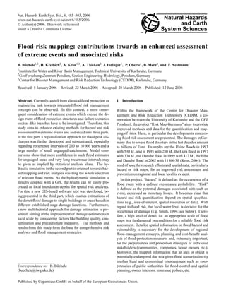
C0 ...C8 regression coefficients 0.00 -1.5
The regression coefficients C0 ...C8 are estimated based
on the gauge-specific flood estimates and the above men- -0.05 -2.0
1 10 100 1000 10000
tioned spatial data sets (available in LfU, 2005b) using recurrence interval T [a]
the method of least squares. The application of this ap-
proach requires two steps. First, MH q is estimated using Fig. 1. Progression of regression coefficients C7 and C8 for recur-
Eq. (1). Subsequently, H QT in unit [m3 /s] is determined rence intervals T from 2 to 10 000 years.
using YT =H qT /MH q in Eqs. (1) and (2):
H QT = YT × MH q × AE0 = YT × MH Q (2) for this specific gauge it may be noticed that the regional-
ization approach is able to reproduce the shape of the sta-
Recently, this approach was extended to recurrence intervals
tistical distribution. At the same time, the 95%-confidence
of 200 to 10 000 years using a selection of 249 gauges and
interval for the statistical distribution (dashed lines) is indi-
applied to a more detailed spatial data set (6200 locations
cating substantial uncertainties, especially in the area of ex-
of the river network, LfU 2005b). The selection of gauges
trapolation (for this sample: about 25% for all H QT with
was done considering the record length and the quality of
T≥100 years). Summing up, the deviations between region-
the flow series in order to achieve more reliable model ad-
alization and flood-frequency analysis vary among the men-
justments for low-frequency events. The present regionaliza-
tioned 249 gauges as presented in Fig. 3. The mean devia-
tion approach is thus consisting of 13 regression equations,
tion is <2.5% at approx. 40% of the gauges, <7.5% at ap-
i.e. one equation for MH Q and each H QT for T from 2 to
prox. 75% and <12.5% at approx. 90%. The deviation is
10 000 years. The coefficients (C0 –C8 ) of these equations
>20% at approx. 3% of the gauges where generally human
are fully documented in LfU (2005b), at which the corre-
activities (e.g., urban drainage systems) or karst conditions
sponding coefficients of determination are R 2 >0.99 for all
are present. Figure 4 illustrates a sample map of the region-
single recurrence intervals (logarithmic analysis). As Fig. 1
alization approach for H q1000 in Baden-W¨ rttemberg. Ac-
u
exemplifies for C7 and C8 (compare Eq. 1), the coefficients
cording to this sample, the highest peak discharges per unit
show a homogeneous progression upon the whole spectrum
area occur in the mountainous regions of the Black Forest
of recurrence intervals, although they are estimated sepa-
(Upper Rhine Basin) and the upper Neckar Basin.
rately for each recurrence interval. To enable user-specific
estimates, the complete spatial data sets and a calculation To substantiate the regionalization approach especially for
tool for the regionalization approach are integrated in a ge- small ungauged catchment areas, the results can be compared
ographical information system (LfU, 2005b), which is dis- to outcomes of rainfall-runoff (RR) models which are sup-
tributed as stand-alone software to local authorities and plan- posed to build on a better representation of catchment char-
ning companies. By these means, regionalized MH Q and acteristics. This was done here for the Fils catchment, a
H QT are provided for any user-defined location of the river tributary to the Neckar River (707 km2 , see Fig. 4), where
network in Baden-W¨ rttemberg, completed by analogous in-
u a RR-model (software see Ihringer, 1999) is available from
formation at 375 gauges and longitudinal profiles for 163 ma- a hydrological study on local flood problems. Within the
jor rivers. Furthermore, the extension of the regionalization RR-model, the catchment is represented by 907 subareas
approach to very high recurrence intervals supports the ongo- and 1501 nodes for the drainage network, considering a to-
ing state-wide elaboration of flood hazard maps and regional tal urban area of 92 km2 , 331 stormwater holding tanks of
dam safety analyses. urban drainage systems and 7 flood-retention basins. As
input of the RR-model, rainfall statistics provided by the
2.3 Model results, comparisons and discussion German Weather Service (DWD, 1997) were used; these
rainfall statistics cover recurrence intervals from 1 to 100
A comparison of at-site and regional flood-frequency anal- years for different duration classes from 0.5 to 72 h. For the
ysis is exemplified in Fig. 2 for the Fils river in Plochin- assessment of higher peak discharges, the mean precipita-
gen showing that the regionalized H QT (squares) are very tion depths for the different duration classes were extrapo-
similar to the statistical distribution for the annual maximum lated. However, different precipitation characteristics (dura-
flood series 1926–2002 (solid line). Beyond the agreement tion classes) cause a set of different flood peaks. Therefore,
www.nat-hazards-earth-syst-sci.net/6/485/2006/ Nat. Hazards Earth Syst. Sci., 6, 485–503, 2006
6. 490 B. B¨ chele et al.: Flood-risk mapping:...extreme events and associated risks
u
0 .0 1 1 0 0 0 0
5 0 0 0
0 .0 5
g a u g e P lo c h in g e n / F ils 2 0 0 0
N o v 1 9 2 6 - O c t 2 0 0 2 ; 7 6 v a lu e s
[% ]
0 .1 0 1 0 0 0
[a ]
5 0 0
e x c e e d a n c e p r o b a b ility
0 .5 0 2 0 0
r e c u r r e n c e in te r v a l T
1 .0 0 1 0 0
2 .0 0 5 0
5 .0 0 2 0
1 0 .0 0 1 0
2 0 .0 0 5
5 0 .0 0 c o n fid e n c e in te r v a l 2
= 9 5 %
L O G - N O R M A L -2
9 5 .0 0 P L O T T IN G P O S
H Q R e g io n a l.
1 2 3 4
1 0 1 0 1 0 1 0
a n n u a l p e a k d is c h a r g e H Q [m ³/s ]
Fig. 2. Comparison of H QT from regionalization (as squares) with flood-frequency analysis at Plochingen/Fils (location see Fig. 4, annual
peak discharges 1926–2002 as plotting positions, Log-Normal distribution as solid line, 95%-confidence interval as dashed lines).
70
MHQ
percentage of gauges (n = 249) [%]
60 HQ2
HQ5
50 HQ10
HQ20
40 HQ50
HQ100
30 HQ200
HQ500
20 HQ1000
HQ2000
10
HQ5000
HQ10000
0
-5 ± 2,5
< -30
0 ± 2,5
5 ± 2,5
-25 ± 2,5
-20 ± 2,5
-15 ± 2,5
-10 ± 2,5
10 ± 2,5
15 ± 2,5
20 ± 2,5
25 ± 2,5
> 30
classified deviation [%]
(regionalized HQT vs. HQT from statistical analysis at gauges)
Fig. 3. Comparison between regionalization and flood-frequency analysis at 249 gauges in Baden-W¨ rttemberg: classified deviations [%]
u
for MH Q and H QT for T =2, ..., 10 000 a (bars from left to right).
the maximum peak of a set representing the relevant spec- eas (especially for H Q1000 <10 m3 /s). The variation around
trum of precipitation characteristics was chosen to estimate the bisecting line, standing for a perfect agreement of both
the 1000-year quantile according of this approach. This value models, can be understood as residual uncertainty of the mu-
is compared to the quantile estimated from the regionaliza- tual application of both models for these specific catchment
tion approach based on observed flood peaks. Figure 5 shows areas. The deviations may be further discussed taking more
a comparison of 1000-year peak discharges of both mod- knowledge on local characteristics into account, that was not
els (H Q1000 from regionalization and RR). According to the yet used in one or both models (e.g., outlets of urban drainage
spatial discretization of the regionalization approach, 265 lo- systems). Mathematically, the deviations between both mod-
cations of the drainage network are plotted. The axes are log- els amount to <7.5% for 66% of all 265 plotted locations,
arithmic in order to visualise the small values better. It can be <12.5% for 82% and >30% for 3% of these locations. The
concluded that the results match fairly well with tendencies latter belong to smaller areas respectively peak discharges
to higher deviations between both approaches in smaller ar- (e.g., 6.96 m3 /s from regionalization versus 11.02 m3 /s from
Nat. Hazards Earth Syst. Sci., 6, 485–503, 2006 www.nat-hazards-earth-syst-sci.net/6/485/2006/
7. B. B¨ chele et al.: Flood-risk mapping:...extreme events and associated risks
u 491
Fig. 4. Regionalized H q1000 in Baden-W¨ rttemberg; location of sample gauge in Plochingen (Fils catchment, 704 km2 ).
u
RR, Fig. 5) where the RR-model – in general – may recog- 1000
nise local influences better. Therefore, more confidence may
be given to the regionalized H QT as implied by statistical
HQ1000 from RR-model [m³/s]
analysis alone (Fig. 2). 100
In view of the needs of practitioners, a coherent and ro-
bust approach for regional flood estimates is thus available
and broadly established in a state-wide sense. Uncertainties 10
of this approach concerning local distinctions call for hydro-
logical justifications of the plausibility of flood estimates on
local scale. The model comparison strategy seems to be the 1
1 10 100 1000
logical way for model validation and practically the unique HQ 1000 from regionalization [m³/s]
chance to reduce uncertainties effectively in areas where the
availability of flow records is scarce. This is valid not only Fig. 5. Comparison of peak discharges calculated by regionalization
in spatial sense (ungauged areas) but also for the extrapola- and RR-model: H Q1000 at 265 locations of the drainage network
tion to very long recurrence intervals. Apart from its practical in the Fils catchment.
use for regional flood estimates, the regionalization approach
leads from at-site flood frequency analysis to distributed hy-
drologic modelling of flood events, enabling a vice-versa re-
view and mutual enhancement of these methods. the flow patterns in a given river section are characterised
by compact and coherent streamlines, 1-dimensional (1-D)
HN-models are considered as adequate for the estimation
3 Hydrodynamic modelling for extreme floods of flood-water levels and delineation of inundation zones
(e.g., Baden-W¨ rttemberg, 2005). In cases with more com-
u
3.1 Basis and objectives plex river geometries and flow patterns (e.g., at river con-
fluences or other complex flow conditions), 2-dimensional
To quantify flood hazard and risk in urban areas or at (2-D) models are used for a spatially differentiated hydraulic
individual locations, flood discharges (e.g., H Q100 ) have analysis, especially when local parameters like flow direc-
to be transformed into hydraulic parameters like water tion, flow velocity, shear stress, etc. are requested. Depend-
levels, inundation depths or flow velocities by means of ing on the intended purposes, both types of models (1-D, 2-
hydrodynamic-numerical (HN) models. In many cases when D) may be applied for stationary flow conditions (e.g., hazard
www.nat-hazards-earth-syst-sci.net/6/485/2006/ Nat. Hazards Earth Syst. Sci., 6, 485–503, 2006
8. 492 B. B¨ chele et al.: Flood-risk mapping:...extreme events and associated risks
u
assessment for a certain H QT ) or unsteady flow conditions tion and validation for a spectrum of (flood) discharges is
(e.g., for impact analyses of dike failures). possible. A detailed description of the system is given by
At the Neckar river (see Fig. 4), the pilot area of this part Oberle (2004).
of the study, a complex flood-information system was set up Areas that contribute to the retention volume of the Neckar
since the late 1990’s (Oberle et al., 2000), consisting of a se- river during a flood event are taken into account by a func-
ries of 1-D- and 2-D-HN-models which are interactively con- tion of storage capacity depending upon the water level. This
nected with a geographical information system (GIS). This function can be determined from the digital terrain model by
system enables the simulation of different flood scenarios in means of several GIS-functionalities and can be verified by
order to evaluate, for example, effects of river engineering comparing calculated with surveyed flood hydrographs.
measures on flood waves. Through its GIS-interface, the hy-
draulic results can be superimposed with a high resolution 3.2 Hydraulic modelling of extreme floods
DTM (grid size: 1×1 m) to determine inundation zones and
respectively the boundaries. The DTM is based on eleva- In most cases, HN-models are applied to documented flood
tion data from different data sources, i.e. terrestrial and air- events from the last decades (in order to assess the present
borne surveys. Apart from topographical information, flood- hydraulic conditions) or to statistical flood events with recur-
relevant spatial data like flood marks, flood impact area, re- rence intervals up to 100 or 200 years (e.g., for delineation
tention zones and legally defined flood areas, are integrated of inundation zones or as design events for flood protection
in the GIS. Linkups to aerial photographs of recent flood measures). With regard to the increasing process complexity,
events complete the volume of spatial data sets. for instance in the case of overtopping or even destruction
With respect to the main target parameters of flood-risk of a flood protection structure, and to the lack of measure-
analysis and mapping (water levels, inundation zones/depths) ments for the calibration and validation of model parameters
and to the flow characteristics along the Neckar river, a gen- for such cases, the application of HN-models to larger floods
erally 1-dimensional HN procedure was chosen. The choice is rarely practised. However, despite of the uncertainties, it
of this procedure was supported by the fact that the handling is necessary to apply HN-models for floods that exceed the
of the system and the computing time should match with the 100- or 200-year level, as they are the most relevant situa-
size of the study area (approx. 220 river kilometres) and the tions in terms of residual risks, causing severe damages and
goal, to install the system as operational tool for daily work- fatalities. In particular with respect to residual risks, it is
ing practice in the water management authorities. Finally, obvious that model parameters should also be valid for ex-
the calculation of a flood event and the visualisation of in- treme events. Only the reflection of all physically plausible
undation depths in the GIS only takes minutes with this sys- hazardous situations from the occurrence of first inundations
tem, so that analyses can be realised also based on actual to the maximum possible water levels yields to a compre-
flood forecasts. Some river sections with more complex flow hensive hazard and risk assessment. This applies equally for
conditions (e.g., tributary mouths) could be assessed only in- flood situations below the design event, as required e.g. for
sufficiently by means of an 1-dimensional approach. Here, cost-benefit-analyses of protection measures or for the as-
local 2-D-HN-models were additionally applied. However, sessment of residual risks due to other failures of technical
a stationary calculation on the base of a 2-dimensional HN or non-technical measures (e.g., late installation of mobile
procedure requires several hours even using a powerful com- protection elements).
puter. Often, historical flood marks indicate much higher water
The hydrodynamic method of the above mentioned 1- levels than current flood protection level and thus, should
dimensional procedure is based on the solution of the serve as realistic reference scenarios for extreme events. In
Saint-Venant-Equations by an implicit difference scheme the upper part of the Neckar, the flood with the highest ever
(Preissmann-scheme, compare Cunge et al., 1980). Under recorded water levels occurred in 1824. The water marks can
the normal flow conditions of the Neckar river, this approach be found at several buildings in flooded communities giv-
is valid and very efficient even for large river sections with ing impressions of the severity of historic floods. They can
respect to data handling, model build-up, model calibration be taken into account for all flood related planning. With
and validation as well as sensitivity analyses and, finally, adapted HN-models (discharge-relevant areas, roughness co-
studies of variants. The functionality of the system includes efficients, etc.) it is possible to assess if similar flood water
modelling schemes for looped and meshed river systems as levels could appear in the present situation.
well as for river-regulating structures (e.g. weirs, groins, wa- The present HN-calculations at the Neckar river have con-
ter power plants). The system geometry of the HN-model, firmed that the historical event 1824 was much higher than
i.e. the discharge area of the main channel and the flood- today’s design flood. Figure 6 shows the calculated maxi-
plains, is represented by modified cross sections. The model mum water levels of the Neckar river for the 100-year flood
calibration is done by comparing calculated water levels with (H Q100 ) and the historical flood of 1824 (under actual hy-
surveyed ones. In most sections, water level measurements draulic conditions). For example, around the community of
of different recent flood events are available, thus a calibra- Offenau, 98 km upstream of the confluence of the Neckar
Nat. Hazards Earth Syst. Sci., 6, 485–503, 2006 www.nat-hazards-earth-syst-sci.net/6/485/2006/
9. B. B¨ chele et al.: Flood-risk mapping:...extreme events and associated risks
u 493
River with the Rhine River, the historical water level of 1824 155.0
Flood marks 1824
was approximately 2.5 m higher than the dikes that have been 154.0 HW 1824
HQ200
built for a 100-year flood. 153.0
HQ100
It has to be emphasised that the consideration of extreme 152.0 HQ50
water level [m asl]
HQ20
historical events can not only support flood awareness as re- 151.0
HQ10
alised scenarios (under historical conditions), but also used 150.0
as reference for the analysis of potential extreme cases un- 149.0
der present conditions. In this regard, the intention here was 148.0
not to reconstruct historical hydraulic conditions or to ver- 147.0
ify historical information in terms of peak discharges. The 146.0
results shown can help, for example, to assess the proba- 145.0
106.0 104.0 102.0 100.0 98.0 96.0 94.0
bility of flood events that cause comparable water levels in Neckar-km
the actual situation. In terms of a reconstruction of histori-
cal discharges, a further investigation on historical hydraulic Fig. 6. Maximum water levels along the Neckar river for statistical
boundary conditions is required (Oberle, 2004). However, flood events H QT with T =10, 20, ..., 200 years) and the historical
due to the limited historical data availability and quality, ma- event 1824 (HW1824), the latter as reconstructed from water-level
jor uncertainties are expected. marks. Note location of the community Offenau at the river Neckar
(98 km upstream of the confluence with the river Rhine).
3.3 Hazard mapping
The above presented hydrological and hydraulic models, and Green, 2000), the largest part of the literature on flood
i.e. the regionalization approach for the estimation of ex- damage concerns direct tangible damage (Merz and Thieken,
treme events (H QT ) as well as the GIS-based flood informa- 2004). The present study is limited to direct monetary flood
tion system for the Neckar river served as basis for the gen- damage to buildings and contents of private households.
eration of hazard maps with prototype character in a state- As outlined above, stage-damage-functions for differ-
wide sense. For example, hazard maps for the lower Neckar ent building types or building uses are an internationally
river (Figs. 4 and 6) are published on the -internet platform accepted standard approach for flood damage estimation.
(Baden-W¨ rttemberg, 2005).
u While the outcome of most stage-damage functions is the
absolute monetary loss to a building, some approaches pro-
vide relative depth-damage functions, determining the dam-
4 Flood-damage estimation
age e.g. in percentage of the building value (e.g. Dutta et al.,
4.1 Basis and objectives 2003). If these functions are used to estimate the loss due
to a given flood scenario property values have to be prede-
Based on the knowledge of accumulated values in the areas at termined (Kleist et al., 2004, 2006). However, using these
risk and relationships between event parameters and resulting functions, one has to be aware that the damage estimation is
damage, flood risks can be identified and quantified, i.e. ex- generally associated with large uncertainties as recent stud-
pected damages for a given flood scenario can be calculated. ies asserted (Merz et al., 2004). One approach to reduce the
This information about flood risk for individual buildings, uncertainty connected with stage-damage functions is their
settlement areas and river basins is indispensable to inform specific adjustment to the area of interest (Buck and Merkel,
the population and stakeholders about the local flood risk, 1999). This strategy was followed here, supported by inten-
for planning of flood control measures and for benefit-cost sive on-site investigations of the building structure in some
analyses of these measures. pilot areas along the Neckar river.
The comprehensive determination of flood damage in- Recent flood events have shown that during slowly rising
volves both, direct and indirect damage. Direct damage is river floods the maximum water level during the flood event
a damage which occurs due to the physical contact of flood is responsible for the resulting damage. In these cases, the
water with human beings, properties or any objects. Indirect gradient of the flood wave is small and for this reason there
damage is a damage which is induced by the direct impact, are no damaging effects due to flow velocity impacts. Ma-
but occurs – in space or time – outside the flood event. Ex- jor damages are caused by wetting of contents and building
amples are disruption of traffic, trade and public services. structure in the cellar and the ground floor. This does not
Usually, both types are further classified into tangible and in- apply for flash floods e.g. in mountainous areas where, due
tangible damage, depending on whether or not these losses to high flow velocity, buildings may collapse partly or to-
can be assessed in monetary values (Smith and Ward, 1998). tally. Therefore, it is obvious that flood damage depends,
Although it is acknowledged that direct intangible damage or in addition to building type and water depth, on many factors
indirect damage play an important or even dominating role which are not considered using stage-damage functions. One
in evaluating flood impacts (FEMA, 1998; Penning-Rowsell factor is the flow velocity, but there are also others like the
www.nat-hazards-earth-syst-sci.net/6/485/2006/ Nat. Hazards Earth Syst. Sci., 6, 485–503, 2006
10. 494 B. B¨ chele et al.: Flood-risk mapping:...extreme events and associated risks
u
duration of inundation, sediment concentration, availability 4.2 Flood damage estimation on local scale based on stage-
and information content of flood warning, and the quality of damage curves
external response in a flood situation (Smith, 1994; Penning-
Rowsell et al., 1994; USACE, 1996). Although a few stud- 4.2.1 GIS-based damage analysis (tool)
ies give some quantitative hints about the influence of some
of the factors (McBean et al., 1988; Smith, 1994; Wind et As discussed above, it is commonly required in flood-risk as-
al., 1999; Penning-Rowsell and Green, 2000; ICPR, 2002; sessment to locate accessible information about hazard and
Kreibich et al., 2005), there is no comprehensive approach vulnerability at a high spatial resolution (e.g. for cost-benefit
to consider these factors in a loss-estimation model. Using analyses, for local protection measures, rating of risks for in-
actual flood damage data from the 2002 flood in Germany, surance purposes). In view of these practical requirements, a
we followed this idea here and developed a multifactorial ap- GIS-based tool for damage estimation was developed in the
proach for damage estimation. present project. This tool supplements the above mentioned
flood information system at the Neckar river, i.e. it builds
The flood-damage estimation can be undertaken on differ- directly on the water level information for individual endan-
ent levels of spatial differentiation: gered objects based on hydrodynamic calculations.
The GIS-based tool for damage estimation on local scale
uses the following procedure.
– On local scale, the damages can be estimated based on
spatial data and stage-damage-functions for individual – Selection of the project area (spatial, postcodes or areas
buildings or land parcels. In Germany, commonly the of communities).
Automated Real Estate Map (ALK) is used for these as-
– Identification and categorization of each building in the
sessments. The ALK data show the base-area of the sin-
project area (based on ALK-Data)
gle buildings and give their specific use (e.g. residential
building, commercial building, stable, garage). – Estimation of the flood-sill for each structure (lowest
damaging water level).
– On a more aggregated level, the approach can be based – Estimation of the ground-floor elevation (floor above
on statistical information about population, added val- the cellar).
ues, business statistics or capital assets for land-use
– Estimation of the values for building-structure and con-
units. These values are published yearly by respon-
tents (fixed/mobile inventory).
sible state authorities (statistical offices). Commonly
data from the Authoritative Topographic-Cartographic – Estimation of the stage-damage-functions, differenti-
Information System (ATKIS) is used for this approach ated for different types of buildings, cellar/floor, build-
in Germany. The ATKIS data differentiate more than ing structure/contents.
100 types of land-use (e.g. residential area, power plant,
sports facilities). – Calculation of the water-level for each object in the area.
– Estimation of the damages to buildings and contents for
different water-levels based upon the type and use of
– Large-scale analyses may be carried out for larger land- each building.
use units, like communities or ZIP-code areas, consid-
ering that they may be only partially flooded. These The tool provides the selection of the project area on the base
analyses are often based on the CORINE land cover of different spatial or administrative areas: barrages, commu-
data (Coordinated Information on the European Envi- nities or postcodes. The area of interest or spatial objects can
ronment). The CORINE data differentiates 45 different be selected from tables or as graphical selection in the GIS.
types of land-use (e.g. continuous urban fabric, indus- For the damage estimation, the water depth close to
trial or commercial units, agro-forestry areas). or inside the object is the determining factor. With the
HN-modelling in connection with the digital terrain model
(DTM) the water depths above the terrain is calculated. The
During the last years, the computational power increased in assumption that the damaging water depth inside the object
a way that today flood damage analyses even for larger river is the same as the depth over terrain is correct if the ground
courses can be undertaken with a high level of detail. In this floor elevation has the same elevation as the surrounding ter-
context, the question of spatial scale of damage analysis is ritory and if there are no protection measures. In this case,
moving from limitations concerning the area size to limita- the relevant elevation of the object basis can be calculated on
tions concerning the quality respectively the level of detail of the base of the DTM as the mean value of the terrain altitude
available spatial data sets. on the buildings base. A second option in the tool is to enter
Nat. Hazards Earth Syst. Sci., 6, 485–503, 2006 www.nat-hazards-earth-syst-sci.net/6/485/2006/
11. B. B¨ chele et al.: Flood-risk mapping:...extreme events and associated risks
u 495
the ground floor elevation and the height of the flood-sill for 1.0
each single object. Thus, local object features and protection 0.9
measures can be considered. 0.8
0.7
The damage estimation is based on the general assump-
damage ratio [-]
0.6
tion that the monetary damage depends on the type and use
0.5
of the building. One of the basic studies was performed by
Linear Polygon Function
0.4
Penning-Rowsell and Chatterton (1977). In the Blue man- Square-root Function, b=0.5
0.3
ual, stage-damage functions for residential buildings in the Square-root Function, b=0.4
0.2 Point-based Power Function C=0.8
UK were derived for age and type of the buildings, the du- Point-based Power Function C=3.0
0.1
ration of the flood event and the social class of the inhabi- User-defined points
0.0
tants. The damages are differentiated for building fabric and 0.0 0.5 1.0 1.5 2.0 2.5
contents. Other similar international studies were done by water depth [m]
Wind et al. (1999); Smith (1994); Parker et al. (1987). In
Germany, in the HOWAS database, some 3600 single dam- Fig. 7. Examples of function types used in the GIS-based damage
age cases for different objects are included. The damage data analysis tool.
were collected after different flood events in Germany. Anal-
yses by Buck and Merkel (1999) showed that for practical
the damage estimation tool as second function type, where
uses, damage estimation with a root function provides rea-
the parameter b is user-defined:
sonable results. √
Due to the fact that the absolute damage depends on a S =b× h (4)
variety of factors being specific for every single building
or land parcel, a meaningful damage estimation can be ex- with S=estimated damage, h=water depth, b=user-defined
pected from the application of such stage-damage functions parameter.
and their adaptation for individual objects or – in terms of The parameter b characterises the damage for h=1 m.
exposure and vulnerability – uniform spatial units. For that Hence, using Eq. (4), the damage progression can be de-
reason, the possibility to apply different functions was imple- scribed with only one parameter. For the sample damage es-
mented in this software module, where the user can choose timation in this paper (see below), the damage functions for
at least one of the three following function types: 1. Lin- different building types in the project area were chosen based
ear Polygon Function, 2. Square-Root Function, or 3. Point- on the flood-damage database HOWAS (Buck and Merkel,
based Power Function. 1999).
– Point-based Power Function
– Linear Polygon Function
In some cases, damage does not occur until the stage rises to
The user interface allows to enter 5 pairs of variates (hi/Si) a threshold height in the building. For example in rooms or
of water-depth and damage, which are interpolated sectional storeys, where floors and walls are tiled, damage can be neg-
with linear functions. Between the minimum (i=1) and max- ligible until the water level affects the electrical installation
imum (i=5) pair, the function can be noted: (power sockets). On the other hand, the maximum damage
is often obtained, when the contents are submerged; a fur-
Si+1 − Si ther rise of the water level does not increase the damage in
S = Si + × (h − hi ) , hi ≤ h < hi+1 (3)
hi+1 − hi a relevant manner. For these cases, a power function can be
chosen in the tool, where the points of first and maximum
where S = estimated damage, Si , hi = user-defined nodes of
damage as well as the exponent C determining the gradient
the function, h=water depth.
of the function can be individually defined.
The first pair of variates (h1 /S1 ) defines the minimum wa-
1
ter depth below which the damage is zero. The last point S0 S0 h − h0 C
(h5 /S5 ) sets the possible maximum damage; for water depths S = Smax × + 1− × (5)
Smax Smax hmax − h0
above the damage stays constant. The Polygon function (3)
allows a simple adaptation to individual damage symptoms with S=estimated damage, h=water depth, (h0 /S0 )=point
of different types of objects. of first damage, (Smax / hmax )=point of maximum damage,
C=user-defined exponent.
– Square-Root Function The three function types (Eqs. 3–5) are exemplified in
Fig. 7.
In practical view, square-root stage-damage functions pro- The creation, editing, and choice of these three functions
vide good results for damage estimation (Buck and Merkel, are realised by different masks that allow the user to con-
1999). Therefore, a square-root function is implemented in veniently handle the input. For the Polygon and the Power
www.nat-hazards-earth-syst-sci.net/6/485/2006/ Nat. Hazards Earth Syst. Sci., 6, 485–503, 2006
12. 496 B. B¨ chele et al.: Flood-risk mapping:...extreme events and associated risks
u
Table 2. Standardized damage to buildings and inundated areas for the test community.
Exceedance Affected buildings [–] Inundated area [m 2 ] Standardized
probability [%] residential total residential settlement damages [%]
10 4 8 4000 6000 0.002
5 14 40 15 000 29 000 0.01
2 71 126 41 000 71 000 53
1 127 242 81 000 129 000 100
0.50 223 378 143 000 220 000 194
0.20 237 403 156 000 237 000 215
0.10 266 447 174 000 267 000 255
0.05 296 496 192 000 298 000 304
0.02 328 540 203 000 326 000 364
0.01 342 571 207 000 341 000 400
Fig. 8. GIS-based damage analysis tool (screenshot of graphical user interface). The damage or the general involvement can be calculated
by selecting the area of interest, land-use and event information and damage-relevant factors.
function types, the damage can be calculated in absolute a range of events, beginning from the flood causing the first
monetary units (EUR) or percentages of damage. damage up to the 1000-year event. The damage values in
Fig. 9 are standardized to the 100-year event. That means for
Before starting the calculation, a flood event must be se-
example, that the damage caused by the 1000-year flood is
lected. According to the coupling of the damage estimation
approximately 2.6 times higher than the one caused by the
tool to the flood information system for the Neckar river,
100-year event.
the outcomes of the hydraulic calculations, i.e. water sur-
faces, can be directly used as input of the damage estimation.
Furthermore, the tool includes functionalities to cope with
The implementation of the damage estimation tool in a GIS-
cases where detailed land-use data (e.g. ALK) are not avail-
software environment is realised in four dialogue modules
able or where the assessment could be simplified. As
shown in Fig. 8.
revealed in Table 2, it is possible to make assumptions
Hence, the GIS-based damage estimation tool enables the e.g. about the number of affected houses in flood-prone ar-
user to assess the flood damage to single buildings in flood- eas, in order to give an overview on flood risk without ex-
prone areas and the spatial aggregation of the event-specific plicitly calculating monetary damage. For damage calcula-
damage for a defined group of buildings or areas. Figure 9 tions on a more aggregated spatial level, the values at risk can
shows the calculated damage values for a test community for be derived from statistical data for administrative districts
Nat. Hazards Earth Syst. Sci., 6, 485–503, 2006 www.nat-hazards-earth-syst-sci.net/6/485/2006/
13. B. B¨ chele et al.: Flood-risk mapping:...extreme events and associated risks
u 497
and related to their spatial unit (EUR/m2 ). In this case, the 10.00
damage estimation can be delivered by spatial intersection
of flood-hazard information (inundation zone) with land-use
exceedence probability [%]
data (e.g. ATKIS) in order to calculate the extension of the 1.00
inundated settlement area (see columns 4 and 5 in Table 2).
Usually, the flood-damage calculation is provided for cost-
benefit analyses of flood protection measures. For this pur- 0.10
pose, the costs of a flood-protection measure can be com-
pared to its benefit, i.e. the avoided damage up to the design
event respectively the residual risk after the implementation
0.01
of the measure, normally expressed as mean annual damage 0.0 1.0 2.0 3.0 4.0 5.0
(MAD). For the above mentioned sample community, a dike standardized damage [-]
designed for a 100-year event provides a significant reduction
of MAD, but the residual risk due to a larger flood event still Fig. 9. Standardized damage to residential buildings in a test
community for annual exceedance probabilities from 0.1 to 0.0001
accounts for approximately 40 percent of the original value.
(i.e. damage to a 100-year flood=1, situation without flood protec-
The main advantage of the presented damage estimation tion measure).
on a local scale is that the damage-determining factors are
given both on the hazard side (being in general the water
depth) as well as on the side of vulnerability (stage-damage a building-specific random sample of households was gener-
functions for individual objects). For estimations on an ag- ated, and always the person with the best knowledge about
gregated spatial level, where areas of the same building type the flood damage in a household was interviewed. An in-
may be defined (e.g. ATKIS-data) but no information on in- terview comprised around 180 questions and lasted about
dividual objects is available, one has to make assumptions on 30 min. The computer-aided telephone interviews were un-
the spatial distribution of buildings and building types. Fur- dertaken by the SOKO-Institute, Bielefeld. Detailed descrip-
thermore, as the water depth in an inundated area varies in tions of the survey were published by Kreibich et al. (2005)
space, the definition of the damage-determining water level and Thieken et al. (2005).
gets more uncertain with increasing spatial units. Thus, us- Statistical analysis was undertaken with the software SPSS
ing stage-damage functions, one has to define the damage- for Windows, version 11.5.1. and Matlab, version 7.0.1.
relevant depth or use a statistical approach to estimate the Since a big share of the resulting data show skewed distribu-
spatial distribution. tions, the mean and the median are given. Significant differ-
ences between two independent groups of data were tested
4.3 Development of a multifactorial approach for damage by the Mann-Whitney-U-Test, for three or more groups of
estimation data the Kruskal-Wallis-H-Test was applied. For all tests a
significance level of p<0.05 was taken.
4.3.1 Damage data of the extreme flood in August 2002
4.3.2 Factors influencing the flood damage
Since flood damage is also influenced by other factors be-
sides the water depth, more knowledge about the connections Flood damage influencing factors can be divided into im-
between actual flood losses and damage-determining factors pact factors like water depth, contamination, flood duration,
is needed for the improvement of damage estimation. There- flow velocity and resistance factors like type of building, pre-
fore, during April and May 2003 in a total of 1697 private ventive measures, preparedness, and warning (Thieken et al.,
households along the Elbe River, the Danube River and their 2005).
tributaries, people were interviewed about the flood damage During the extreme flood in August 2002, for exam-
to their buildings and household contents caused by the Au- ple, contamination led to significantly higher damage ratios
gust 2002 flood as well as about flood characteristics, precau- (fraction of the flood damage in relation to the total value)
tionary measures, warning time, socio-economic variables, to buildings and contents (Fig. 10). The damage ratio of
regional and use-specific factors. The 2002 flood was an ex- contents was increased by 93% for high contamination in
treme event, e.g., with a discharge return period of 150–200 comparison with no contamination. For building damage it
years at the river Elbe in Dresden and with a return period was increased by more than 200%. During the 1999 flood
of 200–300 years at the river Mulde in Erlln (IKSE, 2004). in Bavaria oil contamination on average led to a three times
Detailed descriptions were published by e.g. DKKV (2003), higher damage to buildings, in particular cases even to total
Engel (2004), IKSE (2004). The total damage in Germany is loss (Deutsche R¨ ck, 1999).
u
estimated to be 11.6 billion . The most affected federal state On the resistance side, private precautionary measures sig-
was Saxony where the total flood damage is estimated to be nificantly reduce the flood loss even during an extreme flood
8.6 billion (BMI, 2002; SSK, 2003). In the affected areas, like the one in 2002 (Fig. 11). The damage ratio of contents
www.nat-hazards-earth-syst-sci.net/6/485/2006/ Nat. Hazards Earth Syst. Sci., 6, 485–503, 2006