Engineering Hydrology

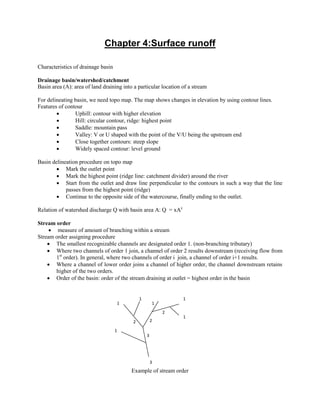
1. Chapter 4:Surface runoff
Characteristics of drainage basin
Drainage basin/watershed/catchment
Basin area (A): area of land draining into a particular location of a stream
For delineating basin, we need topo map. The map shows changes in elevation by using contour lines.
Features of contour
 Uphill: contour with higher elevation
 Hill: circular contour, ridge: highest point
 Saddle: mountain pass
 Valley: V or U shaped with the point of the V/U being the upstream end
 Close together contours: steep slope
 Widely spaced contour: level ground
Basin delineation procedure on topo map
 Mark the outlet point
 Mark the highest point (ridge line: catchment divider) around the river
 Start from the outlet and draw line perpendicular to the contours in such a way that the line
passes from the highest point (ridge)
 Continue to the opposite side of the watercourse, finally ending to the outlet.
Relation of watershed discharge Q with basin area A: Q = xAy
Stream order
 measure of amount of branching within a stream
Stream order assigning procedure
 The smallest recognizable channels are designated order 1. (non-branching tributary)
 Where two channels of order 1 join, a channel of order 2 results downstream (receiving flow from
1st
order). In general, where two channels of order i join, a channel of order i+1 results.
 Where a channel of lower order joins a channel of higher order, the channel downstream retains
higher of the two orders.
 Order of the basin: order of the stream draining at outlet = highest order in the basin
Example of stream order
3
2 2
2
1
11
1
1
1
3

2. Variables based on stream ordering
Bifurcation ratio (RB): ratio of the number Ni, of channels of order i to the number Ni+1 of channels of
order i+1
RB = Ni/Ni+1
RB: relatively constant from one order to another
Length ratio (RL): ratio of average length of streams of order i+1 to that of order i
RL = Li+1/Li
Area ratio (RA): ratio of average area drained by streams of order i+1 to that of order i
RA = Ai+1/Ai
Drainage density (Dd): ratio of total length of all streams of the basin to its area
Dd= Ls/A
 Indication of drainage efficiency
 Higher Dd, quicker runoff, less infiltration and other losses
Length of overland flow = 1/(2 Dd)
Length area relationship (Horton's formula): L = 1.4 A 0.6
where A- mile2
(Useful for large rivers
of the world), L -mile
Stream density (Ds): ratio of number of streams of given order per sq. km.
Ds = Ns/A
Shape of the basin
Shape of the basin governs the rate at which water enters the stream. The shape of basin is expressed by
form factor.
Form factor = average width of basin (B)/axial length of basin (L) = A/L2
Shape factor (Bs): ratio of square of basin length (L) to its area (A), Bs = L2
/A
Slope of the Channel
Slope of channel affects the velocity and flow carrying capacity at any given location at its course.
Slope = elevation difference between 2 points of a channel(h)/horizontal length between points (L)
Centroid of basin
Location of point of weighted center
Hydraulic geometry
It includes the character of channel, longitudinal variation of mean depth, width and velocity at a
particular cross-section.
Stream pattern
a) Meandering types - Formation of successive bends of reverse order leading to the formation
of a complete S curve called meander.
b) Braided - Formation of branches separated by islands

3. c) Straight - Straight and single channel.
Flood plains
The flood plains of a river are the valley floor adjacent to the channel, which may be inundated during
high stage of river. Flood plains are formed due to the deposition of sediment in the river channel and
deposition of fine sediments on the flood plains on flooding.
4.10 Factors affecting runoff
Physiographic factors Climatic factors
1. Basin characteristics
a. Shape
b. Size
c. Slope
d. Nature of valley
e. Elevation
f. Drainage density
2. Infiltration characteristics
a. land use and cover
b. soil type and geological conditions
c. lakes, swamps and other storage
3. Channel characteristics: cross-section,
roughness and storage capacity
1. Strom characteristics
Precipitation: duration,
intensity and magnitude
Movement of storm
2. Initial loss
3. Evappotranspiration
Shape
 Time taken for the water to reach to outlet from remote part depends upon the shape of basin.
 Fan shaped: Greater runoff (same size tributaries, almost similar time of concentration)
 Elongated: broad and low peak (distributed over time)
 Peak flow proportional to square root of drainage area
Size
 Small basin: overland flow predominant
 Large basins: channel flow predominant, constant minimum flow than small basins
Slope
 Slope: control velocity of flow
 Related to overland flow, infiltration capacity and time of concentration of rainfall in streams
 Large stream slope: quicker depletion of storage
 Steeper slope for small basin: higher peak
Elevation
 Affects mean runoff (effect of evaporation and precipitation and effect of snow)
Drainage density
 Drainage density = total channel length/total drainage area
 High density: fast response

4.  Low density: slow response
Land use
 Vegetal cover: reduce peak flow
 Barren land: high runoff
Soil
 Type of soil and subsoil and their permeability conditions
 Geology: Controls infiltration
Storage: reduce runoff
Lakes: reduce flood
Rainfall intensity: increase in runoff with increase in intensity
Rainfall duration: controls volume of runoff
Rainfall distribution: maximum runoff occurs when entire catchment contributes to runoff.
Direction of the storm movement: affects peak flow and time of duration of runoff, up to down: high
runoff, down to up: low runoff
Evapotranspiration: inversely proportional to runoff
Rainfall runoff relationship
Correlation: degree of association between variables.
The relationship between rainfall and runoff is complex due to a number of factors. Therefore, simple
method like correlating runoff with rainfall is used in practice.
a. Linear
Equation for straight line regression
R = aP + b
where R = Runoff
P = Rainfall
a, b: constants
Coefficients by regression
(∑ ) (∑ )(∑ )
(∑ ) (∑ )
∑ ∑
N = number of observations
Coefficient of correlation
(∑ ) (∑ )(∑ )
√[ (∑ ) (∑ ) ][ (∑ ) (∑ ) ]
b. Exponential
For large catchments, exponential relationship can be developed
, m: coefficients
Taking log for linearization

5. With R = lnR, a = m, P = lnP, b = ln , above equation reduces to the one same as before.

6. 4.1 Stream gauging
Streamflow
 That part of precipitation which appears in a stream as surface runoff.
Discharge
 Volume of water flowing through a channel cross section per unit time.
Hydrometry: science of measurement of water
Stage or gauge height
 The elevation of water surface at a location in any water body above a reference datum.
Water body: River, lake, canal, reservoir
Stream gauging station
Stream gauging station is defined as the location at which the river discharges are recorded and the
discharge measurements are carried out.
Purpose of stream gauging: to provide systematic records of stage and discharge
Factors to be considered for the selection of site for stream gauging
 Easily accessible
 Stable and fairly straight river reach about 100m u/s and d/s
 Stable and regular channel bed
 Free from backwater effects
 Regular cross section
 No excessive turbulence and eddies
 No excessive vegetal or aquatic growth
 Velocities: neither too high nor too low, generally in the order of 0.1-5m/s
4.2 Stage measurement
1. Manual or non-recording gauge
Manual gauge is read and recorded by observer/gauge reader once, twice, thrice daily or more. It does not
provide continuous record of stage. It is cheaper and easier to install.
Staff gauge
Staff gauge is the most common and simplest form of manual gauge. It consists of a graduated plate fixed
in the stream or on the bank of river or on a structure e.g. bridge abutment or pier. The level of water
surface in contact with the gauge is measured by matching the reading of the staff and adding with
reference datum level.
It is of three types
 Vertical: one vertical gauge
 Sectional: more than one gauges at different locations
 Inclined

7. Fig. 4.1: Staff gauge
2. Recording gauge or automatic gauge
Recording gauge records continuous stage of a river over time.
Two common automatic gauges
a. Float gauge
A float is connected to one end of a wire which passes through a recorder, and the other end of a rope is
balanced by a suitable counterweight. Displacement of float due to rising or lowering of water level
causes an angular displacement of pulley and hence of the input shaft of the recorder. Mechanical
linkages convert this angular displacement to the linear displacement of a pen to record over a drum
driven by clockwork. The float gauge is protected by installing a stilling well.
Fig. 4.2: Arrangement of float gauge
b. Bubble gauge
Bubble gauge consists of small tube placed at the lowest water level through which compressed air
(usually CO2 or N2 gas) is continuously bubbled out. The pressure required to continuously push the gas
stream out beneath the water surface is a measure of depth of water over the nozzle of the bubble stream.
This pressure is measured by a manometer in the recorder house.
Float
Intake
pipes
Water level
staffga
ugewater
level
Weight
Staff gauge
Intake well
Recorder

8. Fig. 4.3: Arrangement of bubble gauge recorder
4.3 Discharge measurement using velocity-area method
Velocity area method
This involves the measurement of velocity at the gauging site and the corresponding discharge to obtain
river discharge. The velocity is zero at the periphery and changes rapidly as we move from the bank. So a
single area-velocity measurement for the entire cross-section will give highly erroneous results.
Therefore, the cross-section of a river is divided into a number of subsections by imaginary verticals.
Criteria for selection of verticals
 Each vertical should not pass more than 10% of total discharge
 Width of each subsection = 5% of total width of river
 Difference of velocities in adjacent segments: not more than 20%
 Discharge variation between adjacent subsections: between 5% to 10%
For computation of area, the depth of flow is determined by following methods:
 Wading or sounding rod: If the river be crossed, a wading rod is used to measure the depth of
flow. A man walks across the river section with a graduated wading rod to measure water depth.
 Cableway: For deep rivers, cableway is constructed to measure depth and velocity. The lower end
of a cable attached to a current meter with a sounding weight is lowered from cablecar. By
measuring the length of cable lowered, the depth of flow is measured while velocity is recorded
simultaneously by current meter.
 Echo-sounder: In this method, high frequency sound wave is sent down by transducer kept
immersed at the water surface and the echo reflected by the bed is also picked up by the same
transducer. By comparing the time interval between the transmission of the signal and the receipt
of its echo, the distance to the bed is obtained. This method is useful for high velocity streams,
deep streams and mobile or soft bed streams.
Velocity is measured by current meter or floats.
Measurement procedure
Recorder house
Gas pipe
Water level
River bed

9.  Divide the cross-section of the river into n number of verticals.
 At each vertical, measure the horizontal distance from the reference bank, the depth of water and
the velocity at one or more points.
 Compute width, cross-sectional area and average velocity to get discharge at each sub-section.
Computation of average velocity in a vertical
 One point method: for depth<1.0 m
Vav = V0.6d
 Two point method:
Vav = 0.5(V0.2d+V0.8d)
d = depth from water surface
1 2 3 4 5 6 7 8
Fig. 4.4: section for area-velocity method
Computation of discharge
I. Mid section method: widely used
In this method, half width to the left and half width to the right of a vertical is taken as width for a sub-
section.
For section 2 to n-1
Width (Wavi) = ( )
Wi = Width of section i and Wi+1 = width of section i+1
For first and last triangular sections
( )
( )
(Alternative way: Width (Wavi) = ( ) can be used from section 1 to n.)
Cross-section area (Ai) = wavi.di
wheredi = Depth of section i
Discharge at each subsection (Qi) = AiVavi
Total discharge = ∑
II. Mean section method
Cross-section area
( )
Discharge at each subsection

10. ( )
Total discharge = ∑
Moving boat method for discharge measurement in a deep river
Vb= Velocity of boat at right angle to the stream
Vf = Flow velocity
Vr = Resultant velocity
θ = angle made by resultant velocity with the direction of boat
∆t = time of transit between two verticals
Convert surface velocity to average velocity. (Vav = 0.85xVsurface)
Flow
yi+1
Boat
Fig. 4.5: Moving boat method
and
Discharge in each segment
( )
Where
Total discharge = ∑
4.4 Velocity measurement by current meter
1. Current meter
Current meter is the most commonly used instruments for measuring stream velocity. It consists of a
rotating element which rotates due to the reaction of stream current with an angular velocity proportional
to the stream velocity. It is weighted down by lead weight called sounding weight to keep in stable
position in flowing water.
Types of current meter
a. Vertical axis meter
θ
Vf
VR
Vb

11. It consists of a series of conical cups mounted around a vertical axis. The cups rotate in horizontal plane.
The revolutions of cup assembly for a certain time is recorded and converted to stream velocity. The
normal range of velocity measured by such current meter is 0.15m/s to 4m/s. This type of current meter
cannot be used if the vertical component of the velocity is signigicant.
Fig. 4.6: Vertical axis current meter
b. Horizontal axis meter
It consists of a propeller mounted at the end of horizontal shaft.The revolutions of propeller for a certain
time is recorded and converted to stream velocity. The current meter can measure velocity from 0.15m/s
to 4m/s. This type of current meter is fairly rugged and is not affected by oblique flows of as much as 150
.
Fig.4.7: Horizontal axis current meter
Sounding
weight
Stabilizing fin
Cup assembly
Electrical
connection
Sounding
weight
Propeller
Stabilizing finElectrical
connection

12. Relationship between current meter rotation speed and stream velocity
A current meter is so designed that its speed of rotation varies linearly with stream velocity (V). The
relationship is
V = a Ns + b
where V= stream velocity (m/s)
Ns = revolutions per second of current meter
a, b = constants
Calibration of current meter
Determination of constants a and b is known ascalibration of current meter.
Current meters are calibrated in ponds or long channels where water is held stationery. A vehicle with
cantilever arm projection to the channel helps to lower and move the current meter in the pond water. For
each run, the current meter is moved at a predetermined speed (v) and the number of revolutions of the
meter (Ns) are counted. This experiment is repeated over a complete range of velocities and a best fit
linear relation is developed.
Float, types, velocity rod
4.5 Discharge measurement by floats
Floats are used to measure velocity for a small stream in flood, small stream with rapidly changing water
surface and for preliminary analysis.
Vs = surface velocity
L = Distance travelled
t = time taken to travel the float
Discharge = Vav x A
Vav = average velocity = 0.85 to 0.95 times surface velocity
A = cross-sectional area
Types of floats
 Surface float: a simple float moving on stream surface, wooden or metallic object, leaf, orange
 Subsurface float: two floats tied together by thin cord, one float submerged
 Rod float: cylindrical rod partly submerged
Method
 Select straight reach free from current and eddies.
 Measure distance between upstream and downstream section.
 Divide the cross-section into a number of subsections.

13.  For each subsection, release float at an upstream section and note the time taken by float to reach
downstream section. Find average velocity of different sections and compute discharge.
4.6 Slope area method
This is indirect method of discharge measurement. In this method, Manning’s equationand Bernoulli’s
equation are used to estimate the discharge for high floods based on previous flood marks. Two sections
along a river reach are selected. The cross-sectional area of each section and the longitudinal profile
between the sections is measured.
Fig. 4.8: Slope-area method
By using Bernoulli’s equation for sections 1 and 2
Z1, Z2 : Datum headat sections1 and 2
y1, y2 : water depthat sections1 and 2
V1, V2: velocities at sections1 and 2
hL = Head loss
hL = hf + he
hf = Frictional loss
he = eddy loss
Denoting Z + y = h = water surface elevation above the datum
( ) ( ) (a)
From Manning’s equation,
1 2
he
Z2
L
Datum
hf
V2
2
/2g
Z1
y1
V1
2
/2g
y2
Water surface
Energy line
Channel bottom

14. Q =Discharge
n = Roughness coefficient
A = Cross-sectional area
R = Hydraulic radius = A/P where P = wetted perimeter
Sf= Slope of energy line between two points
In other form, Manning’s equation is expressed as
√ (b)
K = Conveyance of channel =
For two sections, average conveyance is
√ (c)
Where and
Eddy loss is given by
| |where Ke = Eddy loss coefficient
Procedure to compute peak discharge by using slope-area method
1. Compute cross-sectional area, wetted perimeter, hydraulic radius, K1and K2 at section 1 and 2.
Compute K using √ .
2. For first iteration, assume V1 = V2. This leads to hf = h1- h2 = Fall in water surface between two
sections. So take hf = h1- h2.
3. Calculate Q using eq. √ √ .
4. Compute V1(= Q/A1) and V2(= Q/A2).
5. Now calculate a refined value of hf by using eq.( ) ( ) ( ) .
6. Take refined value of hf for next iteration and repeat steps 3 to 5until the difference between two
successive values of hf is negligible.
7. Compute Q using final value of hf.
Recommended criteria
 Distance between two sections = 75 times flood depth
 Fall in water head>15 cm
 Straight and uniform reach
 Quality of high-water marks should be good.
Difference between slope-area and velocity area method
I. Velocity-Area method is a direct method for discharge measurement, whereas slope area method is an
indirect method of discharge measurement
II. In velocity-Area method, measurement is performed across a cross-section. The cross-section of a river
is divided into a number of subsections by imaginary verticals. The depth of flow and velocity is
measured at each vertical.
In slope area method, two sections along a river reach are selected. The cross-sectional area of each
section and the longitudinal profile of high flood line between the sections is measured.
III. In velocity-Area method, velocity is measured by current meter or floats. In slope area method,
velocity is computed from the concept of Hydraulics.
IV. In slope area method, the segmental discharge is obtained by multiplying segmental area and mean
velocity, and the total discharge is obtained by summing the segmental discharge.

15. In slope area method, the computation of discharge is based on Manning’s equation and Bernoulli’s
equation.
V. No trial and error is needed in velocity area method, whereas hf is obtained by trial and error approach
in slope area method.
4.7 Flow measuring structures
These structures produce unique control section in the flow. For such structures,
Q =f(H)
Q= discharge
H = Water surface elevation measured from a specified datum
Free flow: flow independent of downstream water level
Submerged or drowned flow: flow affected by downstream water level
Various structures
a. Thin plate structures: made of metal plate, e.g. V-notch, rectangular notch
b. Long base weirs (Broad-crested): made of concrete or masonry
c. Flume: Channel having constriction
Formula
Rectangular notch: √
V-notch: √
Broad-crested weir: √ ( ) and
4.8 Rating Curve (Stage-discharge relationship)
The relationship between discharge (Q) and stage (H) is known as rating curve. Continuous measurement
of discharge is not feasible as it is costly and time consuming. So, discharge data with corresponding
stage is collected from time to time as sample data, and a relation between stage and discharge (rating
curve) is prepared from the sample data. As it is easy and inexpensive, stage is measured continuously.
The rating curve is used to convert the measured stage into discharge. In this way, the continuous
discharge value is obtained.
Q

16. H
Fig. 4.9: Rating curve
Equation of rating curve or stage-discharge relation is expressed in following exponential form.
( )
Q = Discharge
a, b = Constants
H = Stage
H0 = Stage for zero flow
Converting this equation to logarithmic form gives simple linear equation, which is then easy to use for
further analysis.
( )
Or, Y=bX+c
Y =logQ, X = log(H-H0)
The rating curve remains valid so long as the condition at a site remains stable.
Determination of parameters of rating curve
Determination of H0
1. Graphical approach
a. Plot H and Q on a plain graph and draw best fit curve. Extrapolate the curve backwards to touch
ordinate axis where Q =0. Take H corresponding to Q = 0 as H0. Plot Q and H-Ho in log scale and check
whether the plot is straight line. If not, take another value of H0 close to it and repeat the procedure until
straight line plot is obtained.
b. Plot Q vsH to an arithmetic scale and fit the smooth curve. Select three points on the curve such that
their discharges are in geometric progression.
i.e. √
Note H1, H2 and H3corresponding to Q1, Q2 and Q3. Compute H0 by
c. Plot Q vsH to an arithmetic scale and fit the smooth curve. Select three points A, B, and C on the curve
such that their discharges are in geometric progression.Draw vertical lines at A and B and horizontal lines
at B and C. Then two straight lines ED and BA are drawn to intersect at F as show in figure. The ordinate
of F is required value of H0.
H
D
E
C
B
A

17. 2. Determine a, b and H0 simultaneously by least square optimization method.
Value of a and b from regression
(∑ ) (∑ )(∑ )
(∑ ) (∑ )
∑ (∑ )
a =10c
Coefficient of correlation
(∑ ) (∑ )(∑ )
√ (∑ ) (∑ ) √ (∑ ) (∑ )
Methods for extension of rating curve
a. Extension based on Logarithmic plotting of rating curve or using the rating equation
b. Velocity area method: Extend stage-velocity and stage-area curve.
c. Conveyance slope method based on Manning equation:
Flood marks in the river course provides water surface slope of the peak.
√
K = Conveyance of channel =
 For different stages, compute K.
 Compute S for different stages by using from available Q-h data.
 Plot and extend stage-conveyance(K) and stage-slope (S) curve. For different stage, take K and S
from the two curves and compute Q as √ .
Assumptions: For higher stages, the slope remains constant
Control
Control is combined effect of channel and flow parameters, which govern the stage-discharge
relationship.
If the rating curve does not change with time, the control is called permanent control. In other words, the
station with permanent control has single valued rating curve.
If the rating curve changes with time, it is called shifting control.
F
Q

18. Shifting controls
 Vegetation growth, dredging or channel encroachment: no unique rating curve
 Aggradation or degradation in alluvial channel: no unique rating curve
 Variable backwater effect: same stage indicating different discharges
 Unsteady flow effects of rapidly changing stage: for the same stage, low discharge during rising
and high discharge during falling (looped rating)
Correction for backwater effect: To take into account the backwater effect, secondary gauge is installed at
some distance downstream of gauging site and the readings of both gauges are taken. Then, the fall of
water surface in the reach is computed. The relationship for actual discharge (Q) is given by
( )
Q0 = Normalized discharge at the given stage when fall = F0, when the stage in the river is same in both
cases
F = Actual fall
m = exponent 0.5
Unsteady flow correction: Correction has to be applied in case of unsteady flow due to flood wave. The
actual discharge (Q) under unsteady condition is given by
√
Q0 = discharge under steady flow conditions
Vw = Velocity of flood wave
S0 = Bed slope of river
dh/dt = rate of change of stage
4.11 Estimating mean monthly flow for ungauged basin of Nepal
a. Medium irrigation project (MIP) Method
The MIP method presents a technique for estimating the distribution of monthly flows throughout a year
for ungauged locations. For application to ungauged sites, it is necessary to obtain one flow measurement
in the low flow period from November to April.
 In the MIP Method, Nepal has been divided hydrologically into seven zones. Once the catchment
area of the scheme, one flow measurement in the low flow period and the hydrological zone is
identified, long-term average monthly flows can be determined by multiplying the unit
hydrograph (of the concerned region) with the measured catchment area.
 Hydrological zone can be identified based on the location of the scheme in the hydrologically
zoned map of Nepal.
 For catchment areas less than 100 km2
, MIP method is used for better results.
If the measured date is on 15th
of the particular month, the coefficient given in the table is directly used.
For other date of measurement, coefficient for that date is found by interpolation.

19. Monthly flow = April flow x Monthly coefficient
MIP non-dimensional regional hydrographs (Coefficient)
Month Region
1 2 3 4 5 6 7
May 2.60 1.21 1.88 2.19 0.91 2.57 3.50
Jun 6.00 7.27 3.13 3.75 2.73 6.08 6.00
Jul 14.50 18.18 13.54 6.89 11.21 24.32 14.00
Aug 25.00 27.27 25.00 27.27 13.94 33.78 35.00
Sep 16.50 20.19 20.83 20.91 10.00 27.03 24.00
Oct 8.00 9.09 10.42 6.89 6.52 6.08 12.00
Nov 4.10 3.94 5.00 5.00 4.55 3.38 7.50
Dec 3.10 3.03 3.75 3.44 3.33 2.57 5.00
Jan 2.40 2.24 2.71 2.59 2.42 2.03 3.30
Feb 1.80 1.70 1.88 1.88 1.82 1.62 2.20
Mar 1.30 1.33 1.38 1.38 1.36 1.27 1.40
Apr 1.00 1.00 1.00 1.00 1.00 1.00 1.00
Note: all values for mid month

20. Hydrological regions of Nepal for MIP method

21. b. WECS/DHM (Hydest) Method
It is developed for predicting river flows for catchment areas larger than 100 km2
of ungauged rivers
based on hydrological theories, empirical equations and statistics. For long term average monthly flows,
all areas below 5000m are assumed to contribute flows equally per km2
area.
The average monthly flows can be calculated by the equation:
Qmean,(month) = C x (Area of Basin)A1
x (Area below 5000m +1)A2
x (Mean
Monsoon precipitation)A3
.
Where Qmean(month) is the mean flow for a particular month in m3
/s, C, A1, A2 and A3 are
coefficients of the different months.
The catchment area can be calculated from the topographical maps (maps that show contours) once the
intake location is identified.
The input data required in the equation are total basin area (km2
), basin area below 5000m (km2
) and the
average monsoon precipitation (km2
) estimated from isohyetal map.
Values of coefficients for WECS/DHM method
Month C A1 A2 A3
Jan 0.01423 0 0.9777 0
Feb 0.01219 0 0.9766 0
Mar 0.009988 0 0.9948 0
Apr 0.007974 0 1.0435 0
May 0.008434 0 1.0898 0
Jun 0.006943 0.9968 0 0.2610
Jul 0.02123 0 1.0093 0.2523
Aug 0.02548 0 0.9963 0.2620
Sep 0.01677 0 0.9894 0.2878
Oct 0.009724 0 0.9880 0.2508
Nov 0.001760 0.9605 0 0.3910
Dec 0.001485 0.9536 0 0.3607
c. Catchment Area Ratio Method (CAR Method)
If the two catchments are hydrologically similar, then the extension of hydrological data for proposed site
under study could be done simply by multiplying the available long term data at hydrologically similar
catchments (HSC) with ratio of catchment areas of base (proposed site under study) and index (HSC)
stations.
Where, Q = discharge in m3
/s
A = drainage area in sq.km
Suffix 'b' stands for base station and i stands for index station.
This method is useful if the hydro-meteorological data of the index station having similar catchment
characteristics with the base station are available for the data extension.