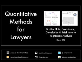
Quantitative Methods for Lawyers - Class #17 - Scatter Plots, Covariance, Correlation & Brief Intro to Regression Analysis

1. Quantitative
Methods
for
Lawyers Class #17
Scatter Plots, Covariance,
Correlation & Brief Intro to
Regression Analysis
@ computational
computationallegalstudies.com
professor daniel martin katz danielmartinkatz.com
lexpredict.com slideshare.net/DanielKatz

2. Associations Among
Variables
Scatterplot is an Initial Tool to Investigate
Relationships Between Variables
Visually Displays Value on the X axis and its
corresponding Value on the Y axis
Roughly Four Possible Relationship Can Be
Revealed in the Data

3. A positive correlation exists between
variable X and variable Y if an increase
in X results in an increase in Y (and vice-
versa)
The more cigarettes you smoke, the
greater the chance of lung cancer.
If you are paid by the hour, the more
hours you work, the more pay you
receive.
The more time you spend studying, the
better grades you make in school.
Scatter Plot
Positive Correlation

4. Scatter Plot
Negative Correlation
A negative correlation exists between
variable X and variable Y if a decrease in
X results in an increase in Y (and vice-
versa).
The heavier your car is, the lower your gas
mileage is.
The colder it is outside, the higher your
heating bill.
The more time you spend watching TV, the
lower your grades are in school.

5. Scatter Plot
No Correlation
In this case, a change in X has no
impact on Y (and vice-versa).
There is no relationship between
the two variables.
For example, the amount of time I
spend watching TV has no impact
on the gas heating bill.

6. Scatter Plot
Non-Linear
The scatter plot illustrates a
nonlinear relationship, in
which Y increases as X
increases, but only up to a
point; after that point, the
relationship reverses
direction.
This is Neg (X^2)

8. Generating Scatter Plots in R
https://s3.amazonaws.com/KatzCloud/auto.dtaLoad this File:
Okay We Are Now Loaded

9. Generating Scatter Plots in R

10. Generating Scatter Plots in R

11. Generating Scatter Plots in R

12. Generating Scatter Plots in R

13. Generating Scatter Plots in R
We Want to Be Able to Color the
Points by {Foreign, Domestic} -
ggplot is probably the best way to
proceed
You Might Consider
Purchasing this Book
http://www.amazon.com/ggplot2-Elegant-
Graphics-Data-Analysis/dp/0387981403

15. Covariance and Correlation
Covariance and Correlation are well established
statistics for identifying and measuring a systemic
relationship between two variables
Covariance Captures how two variables vary in
relationship to each other
Covariance between two variables x / y is measured
as the expectation of the product of each x minus the
population mean and each y minus its population
mean

16. http://ci.columbia.edu/ci/premba_test/c0331/s7/s7_5.html
Covariance
Covariance between two variables
x / y is measured as the expectation
of the product of each x minus the
population mean and each y minus
its population mean

17. http://ci.columbia.edu/ci/premba_test/c0331/s7/s7_5.html
Covariance
Covariance between two variables
x / y is measured as the expectation
of the product of each x minus the
population mean and each y minus
its population mean
Notice the n-1 if sample
(would be n alone if
otherwise)

18. Economic
Growth %
(xi)
S&P 500
Returns %
(yi)
2.1 8
2.5 12
4 14
3.6 10
http://ci.columbia.edu/ci/premba_test/c0331/s7/s7_5.html
Covariance

19. http://ci.columbia.edu/ci/premba_test/c0331/s7/s7_5.html
Covariance

20. Covariance
http://ci.columbia.edu/ci/premba_test/c0331/s7/s7_5.html
Notice
the
“ ... ”
here
Just Showing the
Work for the first
item in the
Summation Series

21. Covariance in R

22. We Have Seen that We Had Covariance Numbers
such as 1.53
This Reveals one of the important limitations of
covariances -- the Units of Covariance are hard to
interpret
Covariance
Typically, Correlation is Reported as it has units that
are scaled and thus allow for easy interpretation
and/or comparison

23. Correlation
Correlation Coefficient is the
statistic that helps us distinguish
b e t w e e n t h e s e t y p e s o f
relationships

24. Correlation
Notice that these are two ways to write the
same formula
Conceptually we are scaling the raw
covariance score to a bench mark unit
and those units are standard deviation
units for x and y
rho

25. Correlation
r is Pearson’s Correlation Coefficient or Pearson’s
Product Moment Correlation Coefficient
Correlation Coefficient is bounded between -1
and +1
Perfect Negative Association r = -1
Perfect Positive Association r = +1
Completely unrelated variables r = 0

26. Correlation
No Hard and Fast Rule about what value for r is
strong enough
Correlation again does not necessarily imply a
causal relationship
See the Murder Rate and Ice Cream Sales
See e.g. Hot Years and Serious and Deadly Assault:
Empirical Tests of the Heat Hypothesis, Journal of Personality
and Social Psychology, Vol. 73(6), Dec 1997, 1213-1223
So Called “Heat Hypothesis” is a likely
confounding variable

27. Correlation

28. Correlation
Lets Look at the Calculation in Detail
sd(mpg) * sd(weight) =
Cov (Weight, MPG) =
same # as before

29. Example Age and Salaries For Technical Workers:
Negative Relationship between age and salaries for
skilled workers
Does not imply that an Age Discrimination Compliant
should be filed
Confound is the diminishing technical skills of older
workers
Tech is a Young Person’s Game
See Daniel l. Rubinfeld, Reference Guide on Multiple Regression, in Reference Manual on
Scientific Evidence 184 (2d ed. 2000)
Spurious Correlation?

30. Welcome to
Regression Analysis

31. Welcome to
Regression Analysis
Regression Analysis is a Tool that Allows for Simultaneous
Consideration of Various Factors/Variables
Allows Researcher to “Control For” the Effect of other
characteristics that might help drive a particular price,
outcome, result, etc.
Regression is VERY LARGE topic and this is a survey course
related to this content:
As stated in Lawless, et al “There will be just a touch of
formality here, but just a touch”

32. Simple Linear Relationships
Y = α + βx
Simple as we are only comparing X and Y
Linear as this is merely a plot of a straight line
Dependent Variable -- Y as it Depends upon the X’s and the
Intercept Term
Independent Variable -- X is independent and it the variable
doing the predicting

33. Simple Linear Relationships
Y = α + βx
α aka “alpha” is the intercept
(this becomes β0 in multiple regression context)
β aka “beta” is the slope of the
regression line
(this becomes β1 in multiple regression context)

34. Here are a Series
of X and Y Values
(Similar to Figure 11-2 Page 302 of
Lawless, et al)

35. Here are a Series
of X and Y Values
(Similar to Figure 11-2 Page 302 of Lawless, et al)

36. Here are a Series
of X and Y Values
(Similar to Figure 11-2 Page 302 of Lawless, et al)

37. Y = α + βx

38. Y = α + βx
Regression Line is Above - it is the Best Fit Line
Regression Seeks to Minimize the Sum of the Squared Differences
between the line of all observations

41. Y = α + βx
Y = 3.2 + .68x

42. Y = α + βx
Y = 3.2 + .68x
Intercept Term
(this becomes β0 in multiple regression context)

43. Y = α + βx
Y = 3.2 + .68x
Intercept Term
(this becomes β0 in multiple regression context)
Regression “Beta” Coefficient
(this becomes β1 in multiple regression context)

44. 05101520 0 5 10 15 20
X
Fitted values Y
Here is that 3.2 Intercept
(i.e. 3.2 on the y Axis)
Y = 3.2 + .68x
Slope Here is .68
for each 1 unit change in X
there is a .68 unit change in Y

45. 05101520
0 5 10 15 20
X
Fitted values Y
Notice that the
prediction line does
not really pass
through the middle
of any particular
observation
There is an error term called “epsilon” which attempts to capture the
amount of error in the model
Y = α + βx + ε
A Large Error Term Mean that the Regression Line Does not Really
“Fit” the Data Particularly Well

46. Multiple
Regression

47. Here is an App
that Predicts the
Price Per Hour of
Various Lawyers
City
Firm Size
Partner
Experience Calculate
Regression Analysis
in Legal Procurement
http://tymetrix.com/mobile_apps/

48. Estimate a lawyer’s rate:
Real Rate Report™ Regression model
From the CT TyMetrix/Corporate Executive Board 2012
Real Rate Report©
$15
1
$16
1
$34
per 10 years$95 +$99
(Finance)
-$15
(Litigation)
n = 15,353 Lawyers
Tier 1
Market Experience
Partner
Status
Practice
Area
Base
+ + +/-
Source: 2012 Real Rate Report™
32
$15
Per
100 Lawyers
Law
Firm
Size+ +
$161
$151
$15
per 100
lawyers $95
$34
per 10
years
-$15
(Litigation)
+$99
(Finance)

49. Y = βo +/- β1 ( X1 ) +/- β2 ( X2 ) +/- β3 ( X3 ) +/- β4 ( X3 ) +/- β5 ( X3 ) + ε
Y = $151 + $15 ( ) + 161 ( ) + 95 ( ) + 34 ( ) +/- β5 ( ) + ε
Per
100
Lawyers
If Tier 1
Market
is True
Partner
Status
is True
Per
10
Years
Practice
Area

50. Daniel Martin Katz
@ computational
computationallegalstudies.com
lexpredict.com
danielmartinkatz.com
illinois tech - chicago kent college of law@