1. ARE CURRENCY WARS WORTH FIGHTING? A PANEL DATA ANALYSIS
Abstract
By analyzing how the exchange rate elasticity of exports has changed over time and across countries, this study
aims to give an answer to a question that has been receiving increasingly media coverage: are currency wars
worth fighting? To this end, the analysis uses a panel data framework covering seven countries over the period
1990-2014, and finds evidence that the elasticity of total exports of goods and services has declined over time.
Introduction
Are currency wars worth waging? Are the risks of retaliations which inevitably follow a competitive devaluation
worth running? This empirical investigation aims at answering these thorny questions by analyzing how the
impact of exchange rates on exports has evolved over time. According to a considerable part of the economic
literature, exchange rates are an important factor in supporting or depressing exports. In particular,
competitively valued exchange rates are regarded as crucial to boost exports. However, in recent years there
have been episodes of large depreciation that seem to have had little impact on exports, one of the most
notable case being Japan. The effectiveness of cheaper currencies in supporting export growth has thus been
called into question by some observers. Have currency depreciations indeed become less effective in boosting
exports?
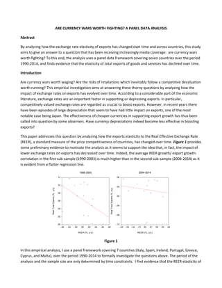
This paper addresses this question by analyzing how the exports elasticity to the Real Effective Exchange Rate
(REER), a standard measure of the price competitiveness of countries, has changed over time. Figure 1 provides
some preliminary evidence to motivate the analysis as it seems to support the idea that, in fact, the impact of
lower exchange rates on exports has decreased over time. Indeed, the average REER growth/ export growth
correlation in the first sub-sample (1990-2003) is much higher than in the second sub-sample (2004-2014) as it
is evident from a flatter regression line.
.00
.02
.04
.06
.08
.10
.12
-.06 -.04 -.02 .00 .02 .04 .06 .08
REER (%, y/y)
1990-2003
RealTotalExports(%,y/y)
-.12
-.08
-.04
.00
.04
.08
-.04 -.03 -.02 -.01 .00 .01 .02 .03 .04
REER (%, y/y)
2004-2014
RealTotalExports(%,y/y)
Figure 1
In this empirical analysis, I use a panel framework covering 7 countries (Italy, Spain, Ireland, Portugal, Greece,
Cyprus, and Malta), over the period 1990-2014 to formally investigate the questions above. The period of the
analysis and the sample size are only determined by time constraints. I find evidence that the REER elasticity of
2. exports has decreased over time. Specifically, the REER elasticity of gross real exports fell in absolute value
from an average 0.63 at the beginning of the period (sub-sample 1, 1990-2003) to 0.4 at the end of the period
(sub-sample 2, 2004-2014). Following the Ahmed, Appendino and Ruta’s approach, I also show that this decline
preceded the global financial crisis, suggesting that it is only in part driven by cyclical factors such as weak
global demand. In short, the effectiveness of cheaper exchange rates to promote exports does appear to have
declined.
Empirical Strategy
To formally investigate the evolution of the relationship between exchange rates and exports, I use panel data
to capture the marginal impact of real exchange rate changes on growth of export volumes, conditional on
country fixed and random effects and other control variables.
I use a panel framework, where annual real export growth is expressed as a function of annual real effective
exchange rate growth. Data are obtained from the IMF database. In my analysis I use three models:
Pooled OLS model (POM): all the observations are pulled together and a ‘grand’ regression is
estimated, neglecting the cross-section and time series nature of the data.
The Fixed Effects model (FEM): all the observations are pulled together, but each cross-section unit is
allowed to have its own intercept.
The Random Effects model (REM): the intercept values are assumed to be a random drawing from a
much bigger pool of countries.
Even though the three models yield similar results, statistical tests suggest that the FEM should be preferred to
the POM, while REM should be preferred to FEM. No matter what model is eventually chosen (based on
statistical tests, economic theory and/or personal beliefs), the conclusion seems to be the same: the role of
exchange rates in promoting exports does indeed seem to be muted. The regression specifications are as
follow:
POM ∆Expit = α + β∆REERit + ξControlit + εit
FEM ∆Expit = α + β∆REERit + ηi + ξControlit + εit
REM ∆Expit = α + β∆REERit + ξControlit + ζit , where ζit = ςi + εit
where ∆Expit denotes real total (goods and services) exports growth of country i at time t, ∆REERit is the growth
in the real effective exchange rate for country i at time t, ηi is the country fixed effects, ςi s the country-specific
error component. The coefficient β captures the effect of depreciation on export growth. I also include a
number of control variables, Controlit, commonly used in the literature. Specifically, 1-period lagged real GDP
(rgdpit) controls for initial conditions, while the export-share weighted average of real GDP growth of each
country’s top five main exports partners (xswgdpit)1
gives a sense of the demand for the country’s exports in a
1
Author’s estimates based on IMF’s World Development Indicators database.
3. particular year. To take into account possible contemporaneous serial correlation among errors, I estimate the
regressions with standard errors clustered across cross-section (White cross-section covariance method). Using
this framework, I run three regressions on seven countries: one for the whole sample (1990-2014), one for the
first sub-sample (1990-2003), and one for the second sub-sample (2004-2014).
Why Panel Data?2
There are several advantages of panel data over cross-section or time series data. Some of them are:
1. Since panel data relate to individuals, firms, countries, etc., over time, there is bound to be heterogeneity in
these units. The technique of panel data estimation can take such heterogeneity explicitly into account by
allowing for subject-specific variables.
2. By combining time series of cross-section observations, panel data give more informative data, more
variability, less collinearity among variables and more degrees of freedom.
3. By studying the repeated cross-section observations, panel data are better suited to study the dynamics of
change. Indeed, it is often of interest (as in this empirical study) to examine how variables, or the
relationships between them, change dynamically (i.e., over time). To do this by using pure time series data
would often require long run of data simply to get a sufficient number of observations to be able to conduct
any meaningful hypothesis tests. But by combining cross-section and time series data (ie, by using panel
data), one can increase the number of degrees of freedom, and thus the power of the test, by employing
information on the dynamic behavior of a large number of entities at the same time.
4. By making data available for several units, panel data can minimize the bias that might result if we
aggregate individuals or firms into broader categories (for example, by averaging values).
In short, panel data can enrich empirical analysis in ways that may not be possible if we use only cross-section
or time series data.
Empirical findings
Table 1 presents my result on the REER elasticity of exports for the whole sample as well as for the two sub-
samples. All three models suggest that the REER elasticity decreased over time. The common constant model
shows that the elasticity of total exports declined by nearly a half, from -0.643 for the period 1990-2003 to
-0.373 for the period 2004-2014. The FEM and the REM models also show a decreasing pattern in the two sub-
samples. Specifically, the FEM shows that the elasticity of total exports fell from -0.629 for the period 1990-
2003 to -0.411 for the period 2004-2014; while REM shows that it dropped from -0.634 for the period 1990-
2003 to -0.378 for the period 2004-2014.
Table 1
Real Growth of Total Common Constant Model Fixed Effects Random Effects
2
Based on Basic Econometrics, Gujarati D.M., Porter D.C.
4. Exports of Goods and
Services
1990-2014 1990-2003 2004-2014 1990-2014 1990-2003 2004-2014 1990-2014 1990-2003 2004-2014
Constant
0.022 0.062** 0.010 0.021 0.074*** 0.009 0.021* 0.067*** 0.010
1.504 2.342 0.770 1.496 2.595 0.691 1.771 3.992 1.534
Real Effective Exchange Rate
-0.595*** -0.643*** -0.373* -0.577*** -0.629*** -0.411* -0.580*** -0.634*** -0.378
-4.786 -2.808 -1.670 -5.131 -2.503 -1.786 -4.395 -4.085 -1.348
1-period Lagged Real GDP
0.259* 0.237 0.090 0.210 -0.339 0.137 0.219 -0.054 0.096
1.879 0.849 0.502 1.392 -1.231 0.604 1.47 -0.189 0.484
Foreign Real GDP
1.139* -0.275 1.554*** 1.214** 0.113 1.581*** 1.202*** -0.048 1.558***
1.891 -0.314 2.732 2.046 0.135 2.621 5.417 -0.101 7.366
Observations 168 91 77 168 91 77 168 91 77
R
2
0.24 0.15 0.45 0.34 0.35 0.49 0.26 0.15 0.45
F-statistic 17.24 5.14 20.14 9.10 4.96 7.10 19.31 5.28 20.30
Redundant FE Rejected Rejected Not Rejected
Hausman test statistic Not Rejected
Not Rejected at
10% Not Rejected
Note: *** indicates statistically significant at 1%, ** indicates statistically significant at 5%, * indicates statistically significant at 10%. Point estimates in bold letters and t-stats below.
White cross-section covariance method for serial correlation robust standard errors.
Why Has the REER Elasticity Declined?
In order to address the possible concern that the lower elasticity is only driven by weaker demand induced by
the global financial crisis, I followed Ahmed, Appendino and Ruta’s methodology and ran three rolling
regressions (one for each model) from the same specification using 7-year windows. Figures 2, 3 and 4 show
that the REER elasticity has gradually decreased since mid-1990s and has only recently started to increase again
(albeit moderately). Importantly, the decline in REER elasticity of exports pre-dates the global financial crisis.
Weaker demand associated to the crisis is, therefore, only one factor among others at play.
6. What can these factors be? In their paper, Ahmed, Appendino and Ruta give four types of explanations:
1. The lower responsiveness of exports to real exchange rates may reflect the fact the global trade growth has
slowed down.
2. Temporary trade barriers such as anti-dumping and countervailing duties are set in response to currency
movements by trading partners.
3. Exchange rate pass-through may have decreased over time. Recent research shows that high performing
firms, large exporters and exporters of high quality goods are more likely to absorb exchange rate
movements in their mark-ups. To the extent that these firms are increasingly more important in the world
trade, we should expect a decrease in the responsiveness of exports to currency depreciations.
4. Countries are more and more integrated in global value chains. As the level of integration increases,
currency depreciation is expected to only improve the competitiveness of a fraction of the value of final
exports. Indeed, Ahmed, Appendino and Ruta’s analysis find evidence that the rise of participation in global
value chains explains on average 40% of the fall in REER elasticity.
Conclusion
This analysis offers further evidence that the REER elasticity of exports has changed over time; in fact, it has
declined. It would be interesting to include more countries in the sample as well as assessing time fixed effects
besides country-specific fixed effects. Declining REER elasticity suggests that there might be fewer reasons to
embark on a currency war as its benefits risk being outweighed by its side effects (which include possible
retaliation from trading partners, higher imported inflation, lower confidence in the stability of the currency,
and reduced central bank’s credibility).