lab 4 requermenrt.pdf
MECH202 – Fluid Mechanics – 2015 Lab 4
Fluid Friction Loss
Introduction
In this experiment you will investigate the relationship between head loss due to fluid friction and
velocity for flow of water through both smooth and rough pipes. To do this you will:
1) Express the mathematical relationship between head loss and flow velocity
2) Compare measured and calculated head losses
3) Estimate unknown pipe roughness
Background
When a fluid is flowing through a pipe, it experiences some resistance due to shear stresses, which
converts some of its energy into unwanted heat. Energy loss through friction is referred to as “head
loss due to friction” and is a function of the; pipe length, pipe diameter, mean flow velocity,
properties of the fluid and roughness of the pipe (the later only being a factor for turbulent flows),
but is independent of pressure under with which the water flows. Mathematically, for a turbulent
flow, this can be expressed as:
hL=f
L
D
V
2
2 g
(Eq.1)
where
hL = Head loss due to friction (m)
f = Friction factor
L = Length of pipe (m)
V = Average flow velocity (m/s)
g = Gravitational acceleration (m/s^2)
Friction head losses in straight pipes of different sizes can be investigated over a wide range of
Reynolds' numbers to cover the laminar, transitional, and turbulent flow regimes in smooth pipes. A
further test pipe is artificially roughened and, at the higher Reynolds' numbers, shows a clear
departure from typical smooth bore pipe characteristics.
Experiment 4: Fluid Friction Loss
The head loss and flow velocity can also be expressed as:
1) hL∝V −whe n flow islaminar
2) hL∝V
n
−whe n flow isturbulent
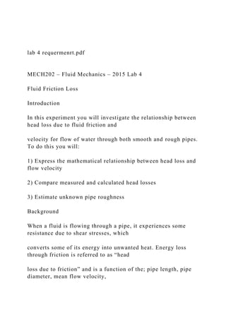
where hL is the head loss due to friction and V is the fluid velocity. These two types of flow are
seperated by a trasition phase where no definite relationship between hL and V exist. Graphs
of hL −V and log (hL) − log (V ) are shown in Figure 1,
Figure 1. Relationship between hL ( expressed by h) and V ( expressed by u ) ;
as well as log (hL) and log ( V )
Experiment 4: Fluid Friction Loss
Experimental Apparatus
In Figure 2, the fluid friction apparatus is shown on the right while the Hydraulic bench that
supplies the water to the fluid friction apparatus is shown on the left. The flow rate that the
hydraulic bench provides can be measured by measuring the time required to collect a known
volume.
Figure 2. Experimental Apparatus
Experimental Procedure
1) Prime the pipe network with water by running the system until no air appears to be discharging
from the fluid friction apparatus.
2) Open and close the appropriate valves to obtain water flow through the required test pipe, the four
lowest pipes of the fluid friction apparatus will be used for this experiment. From the bottom to the
top, these are; the rough pipe with large diameter and then smooth pipes with three successively
smaller diameters.
3) Measure head loss ...
1. lab 4 requermenrt.pdf
MECH202 – Fluid Mechanics – 2015 Lab 4
Fluid Friction Loss
Introduction
In this experiment you will investigate the relationship between
head loss due to fluid friction and
velocity for flow of water through both smooth and rough pipes.
To do this you will:
1) Express the mathematical relationship between head loss and
flow velocity
2) Compare measured and calculated head losses
3) Estimate unknown pipe roughness
Background
When a fluid is flowing through a pipe, it experiences some
resistance due to shear stresses, which
converts some of its energy into unwanted heat. Energy loss
through friction is referred to as “head
loss due to friction” and is a function of the; pipe length, pipe
diameter, mean flow velocity,
2. properties of the fluid and roughness of the pipe (the later only
being a factor for turbulent flows),
but is independent of pressure under with which the water
flows. Mathematically, for a turbulent
flow, this can be expressed as:
hL=f
L
D
V
2
2 g
(Eq.1)
where
hL = Head loss due to friction (m)
f = Friction factor
L = Length of pipe (m)
V = Average flow velocity (m/s)
g = Gravitational acceleration (m/s^2)
Friction head losses in straight pipes of different sizes can be
investigated over a wide range of
Reynolds' numbers to cover the laminar, transitional, and
turbulent flow regimes in smooth pipes. A
3. further test pipe is artificially roughened and, at the higher
Reynolds' numbers, shows a clear
departure from typical smooth bore pipe characteristics.
Experiment 4: Fluid Friction Loss
The head loss and flow velocity can also be expressed as:
1) hL∝V −whe n flow islaminar
2) hL∝V
n
−whe n flow isturbulent
where hL is the head loss due to friction and V is the fluid
velocity. These two types of flow are
seperated by a trasition phase where no definite relationship
between hL and V exist. Graphs
of hL −V and log (hL) − log (V ) are shown in Figure 1,
Figure 1. Relationship between hL ( expressed by h) and V (
expressed by u ) ;
as well as log (hL) and log ( V )
Experiment 4: Fluid Friction Loss
Experimental Apparatus
4. In Figure 2, the fluid friction apparatus is shown on the right
while the Hydraulic bench that
supplies the water to the fluid friction apparatus is shown on the
left. The flow rate that the
hydraulic bench provides can be measured by measuring the
time required to collect a known
volume.
Figure 2. Experimental Apparatus
Experimental Procedure
1) Prime the pipe network with water by running the system
until no air appears to be discharging
from the fluid friction apparatus.
2) Open and close the appropriate valves to obtain water flow
through the required test pipe, the four
lowest pipes of the fluid friction apparatus will be used for this
experiment. From the bottom to the
top, these are; the rough pipe with large diameter and then
smooth pipes with three successively
smaller diameters.
3) Measure head loss between the tappings using the portable
pressure meter for ten different flow
rates by altering the flow using the control valve on the
hydraulics bench for each of the pipes
5. mentioned above. Measure the flow rates using the volumetric
tank or, for small flow rates, use the
measuring cylinder.
4) Measure the internal diameter of each test pipe sample using
a Vernier calliper using the pipe
samples.
Tables to record experimental raw data are provided at the end
of this outline.
Experiment 4: Fluid Friction Loss
Calculations
For your calculations, you are required to provide:
a) Tables showing the raw experimental data
b) Answers to the questions that will be found below:
For the three smooth pipes
Q1) Plot log (hL) vs log ( V ) for the three smooth pipes and
determine n
Q2) Estimate the Reynolds number range for transitional flow
for each of the pipes and comment
what type of flow each of the flow rates is expected to create
for each pipe.
6. Q3) Compare the values of head losses calculated using the
friction factors obtained from the
Moody diagram and Eq.1 to those measured by the portable
pressure meter.
For the rough pipe
Q4) Use the measured head losses and Eq.1 to determine the
friction factor f of the pipe for each
flow rate. Also, calculate the Reynolds number in the pipe for
each flow rate. Plot your values on a
Moody diagram and use them to obtain an estimate for the
roughness (ε) of the pipe.
For all calculations, use water properties at 20 Celsius as
provided in the Moody diagram attached.
Experiment 4: Fluid Friction Loss
Smooth Pipe 1 Smooth Pipe 2 Smooth Pipe 3 Rough Pipe
Diameter
Smooth Pipe 1
Run Measuring Tank
Volume
Measuring Time Head Loss
9. 9
10
Rough Pipe
Run Measuring Tank
Volume
Measuring Time Head Loss
1
2
3
4
5
6
7
8
9
10
__MACOSX/._lab 4 requermenrt.pdf
10. last semester friend similar lab.docx
INTRODUCTION
The purpose of this report is to detail the process and outcomes
of Fluid Friction Experiment. The experiment was conducted to
make students able to better familiarise themselves with the
concept of the head loss due to fluid friction and velocity for
flow of water through smooth bore pipes.
There are three different types of visual flow that will be
shown, laminar, transition and turbulent flow. Laminar flow is
considered a smooth flow where particles move in parallel
straight line. This kind of flow occurs at a very slow velocity.
On the other hand, in turbulent flow particles flow in an erratic
path. This flow occurs at higher velocities. The transition flow
is when there is a significant disturbance in the velocity. This
experiment is done to determine the Reynolds number and that
there is to types of flow may exist in a pipe.
Literature Review:
A weighting function model of transient friction is developed
for flows in smooth pipes by assuming the turbulent viscosity to
vary linearly within a thick shear layer surrounding a core of
uniform velocity and is thus applicable to flows at high
Reynolds number. In the case of low Reynolds number turbulent
flows and short time intervals, the predicted skin friction is
identical to an earlier model developed by Vardy et al (1993).
In the case of laminar flows, it gives results equivalent to those
of Zielke (1966, 1968). The predictions are compared with
analytical results for the special case of flows with uniform
acceleration. It is this case that enables clarifying comparisons
to be drawn with "instantaneous" methods of representing
transient skin friction. (Alan E. Vardy & Jim M.B. Brown,
1995)
Transient conditions in closed conduits have traditionally been
modeled as 1D flows with the implicit assumption that velocity
profile and friction losses can be accurately predicted using
equivalent 1D velocities. Although more complex fluid models
have been suggested, there has been little direct experimental
11. basis for selecting one model over another. This paper briefly
reviews the significance of the 1D assumption and the historical
approaches proposed for improving the numerical modeling of
transient events. To address the critical need for better data, an
experimental apparatus is described, and preliminary
measurements of velocity profiles during two transient events
caused by valve operation are presented. The velocity profiles
recorded during these transient events clearly show regions of
flow recirculation, flow reversal, and an increased intensity of
fluid turbulence. The experimental pressures are compared to a
water hammer model using a conventional quasi-steady
representation of head loss and one with an improved unsteady
loss model, with the unsteady model demonstrating a superior
ability to track the decay in pressure peak after the first cycle.
However, a number of details of the experimental pressure
response are still not accurately reproduced by the unsteady
friction model. (Brunone, B., Karney, B., Mecarelli, M., and
Ferrante, M., 2000)
A new model for the computation of unsteady friction losses in
transient flow is developed and verified in this study. The
energy dissipation in transient flow is estimated from the
instantaneous velocity profiles. The ratio of the energy
dissipation at any instant and the energy dissipation obtained by
assuming quasi-steady conditions defines the energy dissipation
factor. This is a nondimensional, time-varying parameter that
modifies the friction term in the transient flow governing
equations. The model was verified for laminar and turbulent
flows and the comparison of measured and computed pressure
heads shows excellent agreement. This model can be adapted to
an existing transient program that uses the well-known method
of characteristics for the solution of the continuity and
momentum equations. (Silva-Araya, W. and Chaudhry, M.,
1997)
An efficient procedure is developed for simulating frequency-
12. dependent friction in transient laminar liquid flow by the
method of characteristics. The procedure consists of
determining an approximate expression for frequency-dependent
friction such that the use of this expression requires much less
computer storage or computation time than the use of the exact
expression. The derived expression for frequency-dependent
friction approximates the exact expression very well in both
time and frequency domains. Calculated results for a test system
are compared with the experimental results so show that the
approximate expression predicts accurately the surge pressures,
pressure wave distortion as well as pressure attenuation in a
liquid line. (A. K. Trikha, 1995)
From these correlations, a series of more general equations has
been developed making possible a very accurate estimation of
the friction factor without carrying out iterative calculus. The
calculation of the parameters of the new equations has been
done through non-linear multivariable regression. The better
predictions are achieved with those equations obtained from two
or three internal iterations of the Colebrook–White equation. Of
these, the best results are obtained with the following equation:
(Eva Romeo, Carlos Royo, Antonio Monzón, 2002)
· Methodology:
Equipment used:
1. Stop watch
2. Head loss meter
First water was added to the apparatus to initiate the
experiment. The head loss meter was attached to the 10mm pipe
discharge. Then 8 readings were recorded. The time was started
as the water level on the reading apparatus got to 0 litres and
time was then stopped at 2 litre water level. An average flow
was recorded. The same procedure was executed for the second
set of 8 readings but the pipe diameter was increased to
17.5mm. Time again was started at the 0 litre mark and stopped
at the 5 litre mark. In between each reading the flow from the
water source was decreased by closing the valve each time.
13. After the readings were taken flow rate was calculated and then
velocity was calculated.
Formulas used:
This equation was used to calculate flow rate Q, V is the
volume and T was the time that was recorded.
This equation was used to calculated velocity from Q which was
calculated previously and d is the diameter of the pipe that was
being used
Velocity
Flow rate
These equations are the same and are used to calculate the upper
and lower critical velocities.
ρ is the density, u1 and u2 are the upper and lower critical
velocities, µ is the molecular viscosity
14. Results:
The reading abstained from this experiment were tabulated and
further calculations were solved using the following readings.
Figure 2.0
Volume (V) Litres
Time (T) secs
Flow rate (Q) m^3/s
Pipe Dia (dm)
Velocity (u) m/s
Head Loss
Log u
Logh
2
7.97
2.51×10^-4
10mm
3.2
310
0.50515
2.49
2
9.28
2.16×10^-4
10mm
2.75
293
0.439333
2.47
2
9.68
18. 0.176091
1.08
5
20.07
2.5×10^-4
17.5mm
1.04
6
0.017033
0.78
The first set of 8 readings was taken using the 10mm pipe and
the volume of water was 2 litres. The second set of 8 readings
was taken using a 17.5mm pipe and a volume of 5 litres of
water. In both findings the same process was used to calculate
the flow rate, velocity, Log u, and Log h. As the experiment
started the first finding we obtained was the time and head loss,
time was then used to calculate flow rate (Q) also using volume,
the relationship that is seen and is evident through our results in
figure 2.0 is that as time increases flow rate decreases. We were
then able to calculate the velocity as we had the flow rate and
we knew what the diameter of the pipe was, these equations are
shown in the methodology. A total of four graphs were made
from the results two for each set of results these helped
determine Reynolds number (Re) and n-values.
Figure 2.1
Laminar flow
Transition
19. U2
U1
turbulent flow
Figure 2.2
U2
U1
Transition
turbulent flow
Laminar flow
Figure 2.1 and 2.2 show the three zones laminar, transition, and
turbulent. Through this we can determine Re1 and Re2 using u1
and u2 from the graph, ρ density is a constant also µ viscosity is
a constant.
Calculating Re values using figure 2.1
Re1 will have 2 values using u1 and u2
The same proses is used for figure 2.2 to calculate Re2
20. Figure 2.3
Laminar
Turbulent
Figure 2.4
Turbulent
Laminar
From figures 2.3 and 2.4 we got the n values. This was done
using the turbulent
section labelled in the graph.
From figure 2.3 the n value that is the gradient at the turbulent
section was found to be
21. The same procces was repeated in figure 2.4
Discussion
REFRINSE LIST
A. K. Trikha. (1997). An Efficient Method for Simulating
Frequency-Dependent Friction in Transient Liquid Flow.
Available:
http://fluidsengineering.asmedigitalcollection.asme.org/article.a
spx?articleid=1422535. Last accessed 20th May 2015
Alan E. Vardy & Jim M.B. Brown. (2010). Transient, turbulent,
smooth pipe friction. Available:
http://www.tandfonline.com/doi/abs/10.1080/002216895094986
54. Last accessed 20th May 2015.
22. Brunone, B., Karney, B., Mecarelli, M., and Ferrante, M..
(2000). Velocity Profiles and Unsteady Pipe Friction in
Transient Flow. Available:
http://ascelibrary.org/doi/abs/10.1061/(ASCE)0733-
9496(2000)126%3A4(236). Last accessed 20th May 2015.
Eva Romeo, Carlos Royo, Antonio Monzón. (2002). Improved
explicit equations for estimation of the friction factor in rough
and smooth pipes. Available:
http://www.sciencedirect.com/science/article/pii/S13858947010
02546. Last accessed 20th May 2015.
Silva-Araya, W. and Chaudhry, M.. (1997). Computation of
Energy Dissipation in Transient Flow. Available:
http://ascelibrary.org/doi/abs/10.1061/(ASCE)0733-
9429(1997)123:2(108). Last accessed 20th May 2015.
Head loss/ Velocity 2L
0.571.061.341.912.242.642.753.222.061.090.0129.0205.0260.02
93.0310.0
head loss
Head loss / Velocity 5L
1.041.51.792.452.793.083.533.956.011.915.026.032.039.050.05
9.6
velocity m^3/s
head loss
logh/logu 2L
-
0.240.030.130.280.350.420.440.511.341.791.952.112.312.412.4
72.49
log u
log h
logh/logu 5L
23. 0.020.180.250.390.450.490.550.60.781.081.181.411.511.591.71.
78
log u
log h
__MACOSX/._last semester friend similar lab.docx
Last semester friend work similar.docx
Open Channel Flow ReportFluid Mechanics
Table of Contents
1Abstract2
2Experimental Setup3
2.1Objectives3
2.2Apparatus3
2.3Safety Risks3
2.4Method4
3Calculations5
3.1Calculating the ‘Measured’ Flow Rate5
3.2Calculating the ‘Calculated’ Flow Rate5
3.3Measured Head Loss (Between Y1 and Y4):8
3.4Calculated Head Loss (Between Y1 and Y4):8
4Results9
4.1Raw Experimental Measurements9
4.2Calculated Friction, Velocity and Flow Rates10
4.3Calculated Vs Measured Head Loss (Between Y1 and Y4)11
5Discussion12
5.1Accuracy12
5.2Theory and Experiment12
5.3Improvements12
5.4Alternative Experiments13
5.4.1Pipe friction loss in a smooth pipe13
24. 5.4.2Procedure for experimentation14
6Conclusion14
7References15
8Appendix16
1 Abstract
The purpose of this report is to detail the process and outcomes
of our Pipe Friction Experiment. The experiment was conducted
as a means of students being able to better familiarise
themselves with the concepts of energy losses due to friction in
a practical setting. During the experiment we calculated the
head loss due to friction caused by water flowing through a
smooth pipe. We then compared these results to the physical
head loss values we measured using piezometers.
We found that there was an average difference of about 6%
between our measured and calculated values, which we
concluded was an acceptable error most likely caused by failing
in the experimental setup. We would recommend the experiment
be repeated, and the improvements mentioned in the discussion
be implemented to help obtain more accurate results.
2 Experimental Setup2.1 Objectives
The aim of this experiment is to calculate the energy losses
caused by water flowing through a pipe, and to assess their
accuracy through the use of Bernoulli’s equation.2.2 Apparatus
· Elevated water tank
· Water supply
· Pipe (Length: 13.3m, Diameter : 0.019m)
· Mass Scale
· Stop Watch
· Bucket
· Measuring tape (with millimetre increments)
· Five piezometric tubes
· Excess water drainage basin
2.3 Safety Risks
· Slipping on the wet ground surrounding the experimentation
25. area
· Receiving open wounds from sharp edges if equipment was
mishandled
· Falling from ladder due to instability
2.4 Method
1) Set up equipment as shown in diagram:
Figure 1 - Experimental Setup
2) Adjust the height of the exit tube (Ze) to the appropriate
level (First instance was at 1300mm from ground).
3) Record the height of water level in each of the piezometric
tubes, as well as the exit tube height.
4) Place bucket under water output and allow it to fill for
exactly 20 seconds.
5) Measure the mass of the water in bucket and record results.
6) Repeat steps 3 to 5, adjusting the exit tube height (Ze) to
1600mm, 1900mm, 2200mm and 2500mm each time.
7) Calculate the ‘measured’ flow rate by using the recorded
mass and time values. Also the ‘calculated’ flow rate can be
obtained by using changes in height of the exit tube and
26. Bernoulli’s equation.
3 Calculations
3.1 Calculating the ‘Measured’ Flow Rate
The control flow rate was calculating by directly measuring the
volume of water flowing through the system over time:
m3/s
Where is the direct measurement of the flow rate.
Example:
m3/s
3.2 Calculating the ‘Calculated’ Flow Rate
The ‘calculated’ flow rate was measured by deducing the
velocity of the flow and multiplying it by the cross sectional
area of the tube:
m3/s
Where is calculated using Bernoulli’s equation:
Bernoulli’s equation:
This can be rearranged to:
Assumptions:
1) Pentrace = Pexit= 0 (gauge pressure)
27. 2) VEntance= 0
3) ZEntrance– ZExit= H
4) Ve= VPipe (i.e. V is constant throughout pipe)
5) hLoss= hEntrance + hFriction
a. Where
i. K: Loss coefficient
Re-entrant entrance; K assumed to be 0.5
b. And
Example:
If fassumed is originally assumed to be 0.015, then:
Finding the Re based on the estimated velocity:
Finding V using the new value for Re,
Re Calculated:
28. Therefore, V Final:
Re final:
From these results, we were able to calculate the head loss, and
compare theoretical values to the measured results.
3.3 Measured Head Loss (Between Y1 and Y4):
The measured head can be calculated directed by subtracting the
H values at Y4 from Y1.
H at Y1 = 415mm
H at Y2 = 1260mm
Head Loss = 845mm or 0.845m
3.4 Calculated Head Loss (Between Y1 and Y4):
Where:
Distance between Y1 and Y4 = 1960 + 1920 + 2020
= 5900mm
= 5.9m
4 Results
4.1 Raw Experimental Measurements
29. Refer to diagram for meaning of variable:
Figure 2 - Experimental Setup
Collection Tank
Piezometer Tubes
Water from Supply
Large Tank
H
30. Data Set
Ze (mm)
Y1 (mm)
Y2 (mm)
Y3 (mm)
Y4 (mm)
Y5 (mm)
Mass (kg)
Time (s)
1
1300
415
675
955
1260
1515
8.77
20
2
1600
375
590
825
1115
1295
7.85
20
3
1900
335
510
700
945
1055
33. 4.3 Calculated Vs Measured Head Loss (Between Y1 and Y4)
Data Set
H Loss (Measured)
H Loss (Calculated)
Error (%)
1
0.845
0.952
12.7%
2
0.74
0.802
8.4%
3
0.61
0.656
7.5%
4
0.48
0.508
5.8%
5
0.36
0.361
0.3%
5 Discussion
The purpose of this experiment was to highlight friction loss
with respect to flow through pipes. Comparisons were made on
theoretical calculated results against measured results to
determine the validity of the calculated results.5.1 Accuracy
It is important to note that throughout the experiment there were
34. multiple faults in accuracy due to human error and experimental
equipment error. An example of human error would be the
unsynchronised and non-instantaneous reactions from the
individual timing of water flow, and the second individual
holding the bucket under the water output.
A second human error factor would be determining Reynolds
number after obtaining the friction. This was done visually on a
Moody diagram which was not easy to read, and was
additionally limited by its accuracy, which was only to three
decimal places.
Experiential equipment error would be related to how accurate
the mass scale that was being used, the pressure of the input
water supply, the stopwatch accuracy and the measurements of
the equipment such as the height of elevated components.
Data Set
H Loss (Measured)
H Loss (Calculated)
Error (%)
1
0.845
0.952
12.7%
2
0.74
0.802
8.4%
3
0.61
0.656
7.5%
4
0.48
0.508
5.8%
5
0.36
35. 0.361
0.3%
As seen in from the table above, the error was on average
around 6.9%. We believe this was caused by some of the
experimental errors mentioned above and not due to the
theoretical calculations being invalid.5.2 Theory and
Experiment
The aim of this experiment is to determine the friction
experienced by water flowing through a pipe when the entrance
and exit height of the flow were altered. It was assumed that the
velocity is constant throughout the elevation in the pipe
however in the experiment and reality it is known that the water
will travel more slowly due to friction.
The usefulness of the experiment was shown by the similarity of
Qmeasured and Qcalculated. The error margin was small enough
for us to consider the method to be consistent with the theory,
however improving the accuracy of the experiment is still
highly recommended.
5.3 Improvements
Some improvements that can be for the experiment giving a
learning and accuracy advantage would be;
1. Digitally calibrated measuring devices to give accurate
readings by removing human error yielding precise results.
2. Synchronised timer and bucket system to obtain a more
precise measurement once again removing human error and
making results and measurements more accurate.
3. See through equipment to obtain a better understanding of the
experiment and how the flow rate interacts with friction.
4. Repeating the experiment multiple times at the same height
allowing to obtain more insight into the accuracy of each
attempt which can show more stable and reliable measurements,
this also can be applied to the end result.
5.4 Alternative Experiments
36. Figure 3 - Armfield C6-MKII-10 (Faculty UOH n.d.)5.4.1 Pipe
friction loss in a smooth pipe
The apparatus used, as seen above, is the Armfield C6-MKII-10
Fluid Friction Apparatus which is used to study fluid friction
head losses which occurs when an incompressible fluid flows
through pipes, bends, valves and pipe flow metering device.
Water is fed from the hydraulics bench via the barbed connector
(1), as the water flows through the pipes and fittings it is then
fed back into the volumetric tank via the exit tube (23).
The pipes are arranged to provide facilities for testing the
following pipe types (Faculty UOHn.d.):
· An in-line strainer (2)
· An artificially roughened pipe (7)
· Smooth bore pipes of 4 different diameters (8), (9), (10) and
(11)
· A long radius 90° bend (6)
· A short radius 90° bend(15)
· A 45° "Y"(4)
· A 45° elbow(5)
· A 90° "T" (13)
· A 90° mitre (14)
· A 90° elbow (22)
· A sudden contraction(3)
· A sudden enlargement (16)
· A pipe section made of clear acrylic with a Pitot static tube
(17)
· A Venturi meter made of clear acrylic (18)
· An orifice meter made of clear acrylic (19)
· A ball valve (12)
· A globe valve(20)
· A gate valve (21)5.4.2 Procedure for experimentation
1. Fill the network of pipes with water while closing and
opening the appropriate valves to obtain a flow of water through
the desired test pipe.
2. Obtain readings at different flow rates by altering the flow
37. using the control valve on the apparatus.
3. Measure the flow rates using the volumetric tank and measure
head loss between the tapings using a pressurized water
manometer.
4. Repeat experiment for a suitable sample size.6 Conclusion
Our experiment allowed us to find the friction of the flow in the
pipes using Bernoulli’s equation and the theory of energy
conservation. However, the errors present in our method created
some inaccuracies and hence the experiment was not completed
to its full potential. To improve the outcome of this experiment
we would recommend implementing the improvements
mentioned in the discussion.
7 References
ADVDELPhysicsn.d., Moody Chart Calculator, Accessed 1
October 2014
<www.advdelphisys.com/michael_maley/Moody_chart/>
Faculty UOHn.d., Pipe friction loss in a smooth pipe, Accessed
28 September 2014
<http://faculty.uoh.edu.sa/m.mousa/Courses/Thermo-
Lab%20ME%20316/ME%20316_2nd_semester%2012-
13/ME316-2nd-12-13-%20Exps/Exp6-
Pipe%20friction%20loss.pdf>
Huynh, BP, 2008 “Fluid Mechanics – Course Notes”, UTS
Engineering
Neutrium, 2012, Pressure Loss in Pipe, Accessed 20 August
2014, https://neutrium.net/fluid_flow/pressure-loss-in-pipe/
The Engineering Toolbox n.d.Water - Dynamic and Kinematic
Viscosity, Accessed 29 September 2014
<http://www.engineeringtoolbox.com/water-dynamic-kinematic-
viscosity-d_596.html>
38. 8 Appendix
Figure 4 Moody Diagram (Neutrium 2012)
Figure 5 Large Elevated Tank
Figure 6 - Piezometers
Figure 7 - Bucket being weighed on scales
Figure 8 - Water Output
Flow Rate (Measured Vs Calculated)
Q (Measured)Data
Set123450.00043850.00039250.00034050.00028950.000235Q(C
alculated)1.02.03.04.05.00.0004096397410788580.00036972087
79582750.0003343121547147950.0002893962219552910.00024
0121406006494
Data Set
Head Loss (m)
Head Loss Between Two Points (Y1 and Y4)
H Loss (Measured)Data Set123450.8450.740.610.480.36H Loss
39. (Calculated)1.02.03.04.05.00.9524928164900150.802811987315
7870.6564025063463420.5083603181256050.361335450967768
Data Set
Head Loss (m)
Page | 5
__MACOSX/._Last semester friend work similar.docx
results_lab4V1.xlsx
Sheet1Here are the times in seconds for all the pipes for every 5
litres unless specifiedSo the first 4 runs are 5
L0.0050.0030.0020.0010.0001kinematic viscositySP 1 area
m20.0000010040.0000453646Smooth pipe
1D=7.60mm0.0076Flow rate m3/sRun 1Run 2Run 3Run 4Run 5
(3L)Run 6 (2L)Run 7 (1L)Run 8 (100mL)Run 9 (100mL)Run
1Run 2Run 3Run 4Run 5 (3L)Run 6 (2L)Run 7 (1L)Run 8
(100mL)Run 9
(100mL)11.7511.7713.6617.7511.7817.1413.561.654.070.00038
565370.00037096570.00034403670.00028300550.00027615830.
00012514080.00008492570.00006116210.000025109911.511.88
13.1117.7210.1112.8711.61.64.06Velocity
m/s13.314.4114.3617.1412.9817.7611.931.733.838.5012035978.
1774283157.5838145396.2384663726.0875295592.7585559911.
8720697181.3482336960.553512138812.7414.4114.1218.0611.8
912.161.563.97Reynolds
number14.2714.1515.819.3716.189.7364351.7403861900.85178
57407.3610547223.4506346080.9010520881.4995414171.04567
10205.753084189.93252514.2314.2516.149.0515.9611.67Log(V
)2.1402077532.1013777142.026016311.8307343791.806242344
1.0147073510.62704461980.2987953623-0.5914715961Head
loss h_LHead
Loss76.76574.12566.12542.3920.5159.7657.123.8251.68min76.
49. .5250.005027884757828.568.438.769.46666666716.22524851.1
50.80.9750.0012411057039211.7611.4111.587.72333333313.23
72890.690.310.50.0009562220902Rough PipeRunTank Volume
Time 1Time 2Time 3Average timeFlow velocityHL 1 HL
2Average
HLfriction157.857.867.867.8366666675.37261397475.3774.917
5.140.8723420056258.357.87.818.0866666675.54400744474.61
45.9960.30.6574406783357.838.117.638.415.7656763327271.54
71.770.7234846115459.569.299.76106.85573880250.8450.450.6
20.36091130375511.511.1512.9610.317.06826670530.0929.632
9.860.2002861029638.768.2888.95666666710.2340945321.9721
.3321.650.06927011705739.639.838.139.45666666710.8054061
17.2316.3216.7750.04814677597828.938.918.49.78333333316.7
679944910.29.759.9750.011888786529211.3111.5113.057.6066
6666713.037329955.645.415.5250.01089285789
__MACOSX/._Lab-3-Results.xlsx.xlsx
Labs Layout.pdf
MECH202 Fluid Mechanics, 2015, Week 6 Lab Reports
Requirement
Due date:
Weighting: Combined 8% (or 4% each)
For the two reports below, please follow the suggested outline
and formatting included in the
ENGG100 example report that has been provided on ilearn
previously.
50. The specific requirements for each report, and what should be
covered in each section are
outlined below. Please ensure that below the title of your report,
you include your name and
student number. An assignment cover sheet should also be
included.
It is expected that all reports will be typed including any
equations that you wish to include.
Diagrams should be created using graphics software and are not
to be hand drawn. Marks will be
awarded for appropriate formatting and presentation of your
reports.
All work submitted should be the students own work and not be
simply a duplicate of the
information provided. The intention of the two reports is for
students to demonstrate that they
understand how the apparatus and the process connects with the
theory presented in class.
Each lab report will be marked out of a total of 15 marks.
Week 7, Laboratory 3 – Bernoulli’s Principle Lab Report
I. ABSTRACT
51. This should be a concise summary of what was being
investigated, what method was utilised and
the outcome of the experiments. Writing a concise abstract is
challenging, but is necessary to
entice the reader to read the remaining report. This is expected
to be no more than 4 or 5
sentences in length. (1 mark)
II. INTRODUCTION
Describe the problem being investigated in greater detail than
that possible to provide in the
abstract. This should not be greater than one paragraph in
length. (1 mark)
III. METHOD
Describe the process and the equipment that has been used to
obtain the experimental utilising a
diagram as necessary. In total, this section should be no longer
than 1 page in length. (1 marks)
IV. RESULTS AND DISCUSSIONS
52. This is where the results obtained in the lab, the analysis that
has been conducted and the
observations made should be included. For this particular
laboratory, these are expected to be:
1. Provide a table showing the raw experimental results that
were obtained during the
tutorial.
2. Plot the hydraulic grade lines for the five flow rates. What
does this plot tell you about
the interchange of different types of energy as the water flows
through the different
sections of the system (2.5 marks)?
3. Determine the flow velocity at the inlet, outlet and throat for
each flow rate based on
Bernoulli's equation (2.5 mark).
4. For each flow rate, determine the discharge coefficient for
the Venturi meter (Cv) using
the pressure drop between manometers A and E for � (
�
��
+ ℎ). Is Cv a true constant, or
does it vary with Reynolds number? (2.5 marks)
53. 5. Discuss reasons for the difference between the real flow rate
(�����) and ideal flow rate
(������). (1 mark)
6. Identify any potential influences that were not measured or
taken into account. (1
mark)
7. Provide three real world applications of Bernoulli's equation
with correct academic
references. (1.5 marks)
In total, this section should not exceed more than five pages in
length.
V. CONCLUSION
This section should highlight the most significant outcome of
the experiment. This should be no
more than one paragraph in length (1 mark).
54. Week 8, Laboratory 4 – Fluid Friction Loses Lab Report
I. ABSTRACT
This should be a concise summary of what was being
investigated, what method was utilised and
the outcome of the experiments. Writing a concise abstract is
challenging, but is necessary to
entice the reader to read the remaining report. This is expected
to be no more than 4 or 5
sentences in length. (1 mark)
II. INTRODUCTION
Describe the problem being investigated in greater detail than
that possible to provide in the
abstract. This should not be greater than one paragraph in
length. (1 mark)
III. METHOD
Describe the process and the equipment that has been used to
obtain the experimental utilising a
diagram as necessary. In total, this section should be no longer
than 1 page in length. (1 marks)
55. IV. RESULTS AND DISCUSSIONS
This is where the results obtained in the lab, the analysis that
has been conducted and the
observations made should be included. For this particular
laboratory, these are expected to be:
1. Provide a table showing the raw experimental results that
were obtained during the
tutorial.
For the three smooth pipe
1. Plot log(hL) vs log(V) for the three smooth pipes and
determine n. (3 marks)
2. Estimate the Reynolds number range for transitional flow for
each of the pipes and
comment what type of flow each of the flow rates is expected to
create for each pipe
(3 marks).
3. Compare the values of head losses calculated using the
friction factors obtained from
the Moody diagram and Eq.1 to those measured by the portable
pressure meter. (3
marks)
For the three smooth pipe
56. 4. Use the measured head losses and Eq.1 to determine the
friction factor f of the pipe
for each flow rate. Also, calculate the Reynolds number in the
pipe for each flow rate.
Plot your values on a Moody diagram and use them to obtain an
estimate for the
roughness (ε) of the pipe. (3 marks)
For all calculations, use water properties at 20 Celsius as
provided in the Moody diagram
attached.
In total, this section should not exceed more than five pages in
length.
V. CONCLUSION
This section should highlight the most significant outcome of
the experiment. This should be no
more than one paragraph in length (1 mark).
__MACOSX/._Labs Layout.pdf
57. Last semester friend report bit diffrent.docx
2
Introduction:
The Bernoulli’s principle states that the fluid speed is inversely
proportional to the pressure or the potential energy for a non-
conducting inviscid flow of fluid. Bernoulli Principle is named
after the Dutch-Swiss mathematician Daniel Bernoulli.
Bernuolli’s theorem usually relates to Bernuolli’s equation he
expression of the Bernoulli's equation is as follows:
Figure1
The experiment’s objective is to investigate the validity of
Bernoulli’s Theorem as applied to the flow of water in tapering
circular duct. Bernoulli’s theorem is based on the conservation
of mass and energy in the fluid flow. The report first represents
the literature review of the experiment. The report then explains
the method and findings of this experiment. The values
computed are then compared with the measured values to
determine the validity of the Bernoulli’s principle.
Literature Review:
In Bernoulli’s theorem, the fluid is considered incompressible
and has no viscosity. The fluid is taken to be flowing through a
pipe with a cross-sectional area and pressure such that an
element is moved a distance . The theorem states that the sum
of pressure, the potential, and kinetic energy per unit volume is
equal to fixed constant at any point (Giambattista, Richardson
and Richardson, 2010).
Where p is the pressure, is the density of water in this case, g
is gravitational acceleration, h is height, and v is the velocity.
This is considered on one side of the pipe. After dividing this
58. equation by the viscosity, .
Constant
Where is the pressure head, is the velocity head, and the whole
equation is the piezometric head (Oertel, 2004).
Application of the Bernoulli's principle to various fluid flow
types results in what is referred to as the Bernoulli’s equation.
The Bernoulli’s equation forms differ depending on the types of
flow. The simple Bernoulli's principle is applied to
incompressible flows. For compressible flows at higher Mach
numbers, more advanced forms of the Bernoulli equation are
applied.
To understand Bernoulli's Principle, the best way is through
grasping the energy conservation principle. The energy
conservation principle states that the aggregated energy would
be the same for an ideal fluid or any cases where effects of
viscosity are neglected. The energy conservation principle
clearly simplifies Bernoulli's equation, which then deliberates
itself and states that all forms of energy in total would be the
same. As a result, it could be validated through multiple
calculations, which has been achieved by the fluid scientists. It
is very important for the system to be a steady flow (Oertel,
2004).
The principle can also be directly derived from Newton’s
second law. If a small fluid volume is flowing horizontally from
a high-pressure region to a low-pressure region then the
pressure in front is will be less than behind. This gives the
volume a net force, and there is acceleration along the
streamline. Fluid particles are subject to only weight and
pressure. If a fluid is horizontally flowing along a streamline
section, the velocity will increase only when the fluid on that
section moves from a higher-pressure region to a lower pressure
region (Mulley, 2004).
Bernoulli's theory has many implementations in everyday uses;
more specifically in pipes and infrastructure uses. The
59. Bernoulli’s equation is applied when given velocities at two
points of the streamline and pressure at one point. In such a
case, Bernoulli's Equation could be used to determine the
unknown pressure. An example of such a case is the flow
through the converging nozzle.
Several equipment are used in analyzing the Bernoulli's
equation that has been implemented in the real world. For
instance, the pitot probe for the total pressure considered as the
head hT of the fluid in a short distance upstream of the probe's
tip. Also, the valve needs to be controlled gradually to stabilize
the dihydrogen monoxide level in the manometer (Mulley,
2004).
Methodology
The following apparatus are required to perform the experiment:
1. Hydraulic Bench: This allows flow by timed volume
collection to be measured.
2. Bernoulli’s Apparatus Test Equipment.
3. A stopwatch for timing the flow measurement
The first step is ensuring that the Bernoulli apparatus on the
hydraulics bench is leveled. The manometer is carefully filled
with water to eliminate air pockets from within the pipes to
ensure no obstruction that occurs in the resulting reading
obtained. The inlet feed and control valves were adjusted prior
to the start of the experiment for convenience and to obtain
correct reading for the difference between highest and lowest
manometer levels. Three readings were recorded to obtain an
average discharge.
Equations used:
Velocity=discharge/area
60. Results and Discussion:
Table 1: Discharge (Flow rate)
Observation No
Volume (L)
Time (seconds)
Flow rate (mm^3/sec)
Average Discharge (mm^3/sec)
1
3
30.37
0.098
99044
2
3
30.37
0.098
99044
3
3
64. 207
F
135
201.76
2.07
15
542.49
150
149.99
Table 4: The Dimension of cross section
Tapping Position
Manometer Height
Diameter of cross-section (mm)
A
h1
25
B
h2
13.9
C
h3
11.8
D
h4
10.7
E
h5
10
F
h5
25
The results obtained from the experiment are used to determine
the validity of the Bernoulli’s principle. Comparison of the
values of the measured and calculated head is used to verify the
65. principle. The total head cannot be calculated directly without
first finding the velocity and the static head. The velocity
requires to be calculated from the cross-sectional area and the
discharge. The static head is obtained from the manometer
reading.
Table 1 shows the results obtained in getting the average
discharge by measuring the flow rate and the time. The average
discharge was obtained as 9904mm3/sec.
Table 2 shows the readings from the manometer for each tube.
The readings obtained include the tube diameter that is used to
get the cross-sectional area, the manometer level, the probe
level and the probe distance. These values are used in the
calculations in Table 3 to obtain the total heads.
From the given formulas, Table 3 was generated. The table
shows the calculated and the measured values of the velocity
and the head. Comparing the values of the calculated and
measured total heads, it is clear that for all the tubes, the values
are similar. There are only negligible disparities in some of the
values, for example, in tube B the measured total head is
210mm while the calculated total head is 209.99mm. The values
are used to determine the validity of the Bernoulli’s principle.
Table 4 shows the diameters of the tubes and their tapping
points. The diameters are used to assist in obtaining the cross-
sectional area that is required in the calculation of the velocity.
The experiment’s purpose was to investigate the validity of
Bernoulli’s Theorem. Comparisons were made with the
theoretically calculated result against measured results to
determine the validity of the Bernoulli’s equation. From Table
3, the values of the calculated, and the measured total head for
all the tubes were identical. From these values, it can be
concluded that the Bernoulli’s principle is valid. It is important
to note that throughout the experiment there were various errors
caused by human and experimental errors.
References
Brewster, H. (2009). Fluid mechanics. Jaipur, India: Oxford
66. Book Co.
Chanson, H. (2004). Environmental hydraulics of open channel
flows. Oxford: Elsevier Butterworth-Heinemann.
Giambattista, A., Richardson, B. and Richardson, R. (2010).
College physics. Boston: McGraw-Hill.
Enrique Zeleny, (2015), BernoullisTheorem [ONLINE].
Available at:
http://demonstrations.wolfram.com/BernoullisTheorem/
[Accessed 12 May 15].
Mulley, R. (2004). Flow of industrial fluids. Boca Raton, Fla.:
CRC Press.
Oertel, H. (2004). Prandtl's essentials of fluid mechanics. New
York: Springer.
__MACOSX/._Last semester friend report bit diffrent.docx
last semester friend report2.docx
Flow Measurement ReportFluid Mechanics
Table of Contents
Table of Contents2
1Abstract3
2Experimental Setup3
2.1Objective of Experiment3
2.2Apparatus3
2.3Risks4
2.4Method4
2.5Diagram of Setup and Photos5
2.6Theory (Formula)6
2.6.1Orifice Plate:7
2.6.2Flow Nozzle:8
2.6.3Venturi:9
2.7Results10
3Discussion11
67. 3.1Explanation of each device11
3.1.1Geometry:11
3.1.2How they measure pressure:12
3.1.3Differences in Accuracy:12
3.2How our results fit with these:13
3.3Experimental Error14
3.4Relative energy costs (in terms of pressure drops across each
device)15
3.5Relative Advantages and Disadvantages of each device16
3.5.1Orifice plate:16
3.5.2Flow nozzle:16
3.5.3Venturi:16
3.6Other methods that measure flow17
4Conclusion17
5References18
6Appendix18
6.1Appendix 1:18
6.2Appendix 2:19
Abstract
This report outlines an experiment that was designed to
determine the accuracy of three different devices when they
measured the flow rate of a fluid through a cylindrical pipe.
These three devices were the Orifice plate, Venturi and Flow
nozzle.
As the fluid flowed from the source to a volumetric tank it was
forced to go through the Venturi, Nozzle and Orifice. Through
the use of a differential pressure transmitter, the individual
pumps were able to change in pressure for the calibrated
devices and hence calculate flow rates.
Upon applying the data recorded in the experiment, it was
calculated that the orifice provided a flow rate of. The Venturi
yielded a flow rate of while the nozzle had a flow rate of. These
were compared to the measured flow rate of.
It was initially assumed that the Orifice would be the least
accurate device, while the venture would be the most accurate.
68. The presumption of the orifice plate being the least accurate of
the three devices was correct. However the second presumption
was disproved through the experiment as the nozzle
unexpectedly had the most accurate flow rate.
However this result was due to the multitude of errors present
within the experiment and hence it is suggested that the
experiment is repeated once the faults have been
corrected.Experimental SetupObjective of Experiment
This experiment aims to measure the flow rate of water through
a circular pipe with the use of three different measuring
techniques. Through an analysis of the measurement techniques,
individuals will be able to determine the various advantages and
disadvantages of each method. Apparatus
· Water Supply
· Venturi
· Orifice
· Nozzle
· Flow regulating valve
· On-off Valve
· Volumetric tank
· Drain
· Differential pressure transmitters
· Stopwatch
· Power supply
· Ammeters
Risks
This experiment presents a variety of risks to individuals either
participating or observing.
The first is a leakage of water, which can happen through
broken pipes, improper connections or a defective volumetric
tank. These risks can result in slippage or damage to
surrounding equipment. This can be prevented by testing all
69. components prior to the experiment, and replacing all defective
parts.
Rusting equipment is also a major risk within this experiment.
Failure to appropriately maintain and manage equipment may
result in rusting that can deem it unable to fulfil its use. Hence
surrounding equipment can be waterproofed to prevent any
damage. Furthermore getting rust into open wounds and eyes
can be extremely harmful. Therefore individuals must wear
gloves, lab coats and safety goggles to prevent harm.
Electrical safety is one of the most important considerations
when undertaking this experiment. This experiment presents the
potential for a water and electricity mix which can be extremely
harmful and result in electrocution. Therefore individuals must
dry their hands before dealing with electrical equipments and
follow appropriate procedures.
Method
1. Before beginning the experiment it is important to calibrate
each device as shown in the graphs in Appendix 1 to minimise
errors in the experiment.
2. The experiment is set up as shown in the diagram below.
3. Then a Differential Pressure Transmitter in conjunction with
a power supply and ammeter is connected to each the orifice,
nozzle and venturi.
4. The water is supplied at a steady rate and simultaneously the
stop watch is started
5. The volumetric tank is filled to 100 litres and the time is
recorded.
6. Average the data in each column after every three trials
7. With the recorded data, gather the pressure drop, and
calculate the flow rate.
8. The volumetric tank is emptied ready to repeat the
experiment again at different flow rates for a total of three sets
of flow rates.
9. Compare measured flow rates with the calculated flow rates
70. to deduce the accuracy in each device.
10. Use the stopwatch as the control experiment, and have the
differential pressure transmitter as the actual experiment.
Diagram of Setup and Photos
Figure 1: Third measuring device the venturi used in the
experiment.
Figure 2: Nozzle flow device used in the experiment.
Figure 3: The orifice plate utilised during the experiment.
Figure 4: Experimental Setup and Arrangement for measuring
pressure difference (Huynh 2008)
Theory (Formula)
The measured flow rate for the experiment can be found by
using the equation below:
When:
V = volume of fluid (100 litres)
T = average time (49.33 seconds)
This is then compared with the calculated flow rate values of
the orifice, nozzle and venturi to deduce the accuracy of the
devices in measuring the flow rate of a fluid.
Orifice Plate:
71. All the Calculation shown in the appendix
· For all three devices finding the pressure is necessary in
determining the flow rate as it is needed in the final equation
which determines the Qcalculated value for the devices. This
can be acquired by using the equation in the corresponding
graph found in appendix 1.
Where:
mA = average milliamps recorded on multimeter (9.09)
P = Pressure
· The area is also needed to calculate the flow rate of the
devices. For the orifice, only one area is needed.
Where:
A = area with respect to d.
r = radius (0.0125 meters)
· This ratio is needed in order to extract necessary information
from the graph in appendix 2.
Where:
d = orifice diameter (25 millimeters)
D = pipe diameter (52.6 millimeters)
· Using the d/D value and assuming a high Reynolds number
(Re) of 2 x 10⁵, a coefficient can be found of Cv= 0.64 from
graph in appendix 2.
· The flow can be calculated by using the equation:
Where:
Qcalculated = calculated flow rate
Cv = orifice coefficient (0.64)
A = area (4.91 x 10⁻⁴ m2)
72. ΔP = average pressure (14261.6 Pa)
Ρ = density of fluid (1000 kg/m3)
Flow Nozzle:
All the Calculation shown in the appendix
· Solving for the pressure by using the nozzle graph in appendix
1 yields. (Average P)
Where:
mA = average milliamps recorded on multimeter (10.546)
P= Pressure
· Calculating the area for both the pipe and nozzle diameter
Where:
A1 = area of the pipe
r = radius (0.0263 meters)
Where:
A2 = area of the nozzle
r = radius (0.01 meters)
· Calculating the diameter ratio gives.
Where:
d = nozzle diameter (20 millimetres)
D = pipe diameter (52.6 millimetres)
· Using the d/D value and assuming a high Reynolds number
(Re) of 2 x 10⁵, a coefficient can be found of Cv= 0.985 from
the graph
73. · The flow can be calculated by using the equation:
Where:
Qcalculated = calculated flow rate
Cv = Nozzle coefficient (0.985)
A1 = area of pipe (2.17 x 10⁻³ m2)
A2 = area of nozzle (3.14 x 10⁻⁴ m2)
ΔP = average pressure (17690.7Pa)
ρ = density of fluid (1000 kg/m3)
Venturi:
All the Calculation shown in the appendix
· Solving for the pressure by using the Venturi graph in
appendix 1 yields.
Where:
mA = average milliamps recorded on multimeter (10.186)
P= Pressure
· Calculating the area for both the pipe and venturi diameter
Where:
A1 = area of the pipe
r = radius (0.0263 meters)
Where:
A2 = area of the venturi
r = radius (0.0102 meters)
· Calculating the diameter ratio gives.
Where:
d = venturi diameter (20.35 millimetres)
D = pipe diameter (52.6 millimetres)
· Using the d/D value and assuming a high Reynolds number
74. (Re) of 2 x 10⁵, a coefficient can be found of Cv= 0.975 from
the graph
· Likewise with the venturi the flow can be calculated by using
the equation:
Where:
Qcalculated = calculated flow rate
Cv = Venturi coefficient (0.975)
A1 = area of pipe (2.17 x 10⁻³ m2)
A2 = area of nozzle (3.25 x 10⁻⁴ m2)
ΔP = average pressure (14682.4Pa)
ρ = density of fluid (1000 kg/m3)
Results
Nozzle
Orifice
Venturi
d (mm)
20
25
20.35
Area d (mm2)
0.0003142
0.0004909
0.0003253
D (mm)
52.6
52.6
52.6
Area D (mm2)
0.002173
0.002173
75. 0.002173
d/D
0.38
0.48
0.3868821
d*D (mm2)
1070.41
Cv
0.983
0.640
0.973
Table 1: Dimensions for the flow devices used along with their
corresponding coefficient values.
Table 2: Recorded multimeter readings for the devices after
nine trials.
Table 3: Average recorded result from the experiment
Table 4: Error comparison of devices And Average Flow rate
Figure 5: Pressure drop across device vs. measured mass flow
rate
Table 5: Orifice related calculation
Figure 6: Measured mass flow rate vs. calculated mass flow rate
for Orifice
76. Table 6Venturi related calculation
Figure 7: Measured mass flow rate vs. calculated mass flow rate
for Venturi Meter
Table 7 Nozzle related calculation
Figure 8: Measured mass flow rate vs. calculated mass flow rate
for Nozzle
Figure 22
Table 8: Shows the measured and calculated flow rates for the
devices along with their average pressures.Discussion
Explanation of each device
Geometry:
Orifice Plate: The orifice plate consists of a main cylindrical
pipe roughly 52.6mm in diameter along with two thin plates
located about halfway through the pipe. The plates extended
into the pipe from either side leaving an orifice in the centre of
the pipe of about 25mm in diameter which is roughly half of the
original diameter. The plates also consist of 45 degree bores
which provide a sharper edge for the plates.
Figure 5: Orifice (Munson 2013)
Nozzle: This flow measuring device is made up of a funnel inlet
that is designed to impede regular flow and measure pressure.
This funnel inlet decreases in diameter from 52.6mm to 20mm
to create less turbulence when the fluid exits the device.
77. Figure 6: Nozzle Munson 2013)
Venturi: Being the most complex out of the three devices the
venture produces a contraction in the pipe which is shaped like
an hour glass. The contraction leading to the centre of the
venturi is not equal on both sides. In the experimental setup the
venturi had a declined slope of 20 degrees on the entry side of
the flow and a decline of 5 to 7 degrees on the exit side. The
funnel decreases from a maximum of 52.6mm to 20.35mm.
Figure 7: Venturi (Munson 2013)
How they measure pressure:
Since the drop in pressure is used to measure the flow rate, it is
important to have an understanding of Bernoulli’s equation.
Figure 8: Princeton 2008
Orifice:
As fluid begins to flow, the velocity around the orifice plate
increases due to the restricted cross section. Through the
formula we see that change in pressure is proportional to the
square of the velocity. Hence the increase in final velocity
results in a decrease in pressure. Two separate tubes on either
side of the orifice are connected to a differential pressure meter
to measure the change.
Nozzle:
As fluid begins to flow, the velocity increases due to the
decreasing cross section and results in a drop in pressure due to
the same formula applicable to orifice. Similar to the orifice,
two separate tubes across the nozzle measure the change in
pressure.
Venturi:
The venturi was built to further reduce turbulence within flow
78. measurement. To do this it eliminates restrictions by the flow
measurement device and simply has a slowly decreasing
diameter, and again the pressure is determined through two
tubes across the device which is connected to a differential
pressure meter.
Differences in Accuracy:
Firstly from the designs developed for each device we can see
the varying amounts of turbulence. The orifices design is built
in such a way, that the fluid is required to quickly adapt to a
changing diameter and hence there is a significant amount of
turbulence after exiting the orifice. Therefore in theory the
Orifice is very inaccurate.
Secondly the Nozzle is built to allow the water to adjust to the
changing diameter. Despite this design, as the water exits the
device there is turbulence, and hence a loss in pressure.
However due to the inlet, there is less turbulence and hence less
pressure loss in comparison to the orifice.
Lastly the Venturi is built in such a way that it alleviates
turbulence extensively and allows pressure drops to mainly
occur due to the changing diameter. However unlike the Nozzle,
this is done as the water both enters and exits the device. Hence
in theory the venturi should be the most accurate way of
measuring the flow rate.
Expected results due to theory
Device
Accuracy Ranking (Most Accurate to Least Accurate)
Venturi
1
Nozzle
2
Orifice
3
79. Table 9: Expected Results Due to theoryHow our results fit with
these:
Table 9: Results
Firstly, aligning with theory, the results indicate that the orifice
is indeed the least accurate way of measuring flow rate. This is
highlighted through 5.96%,3.3%, and 15.8% errors across the
three flow rates and is clearly further away from the actual flow
rate than both the nozzle and venturi. However observing these
results alone cannot ensure their validity, and hence we must
analyse both the nozzle and venturi.
In this section of the results both the venturi and nozzle do not
seem to follow theory. Through an analysis of the results, it can
be determined that across the board the nozzle seems to be
significantly more accurate than the venturi. This is most
clearly highlighted through the measured flow rate of 1.38,
where the nozzle has 2.8% error in comparison to that of 27%
for the venturi. This leads us to question the method and
whether results have been skewed due to experimental error.
Results analysis
Device
Accuracy Ranking (Most Accurate to Least Accurate)
Venturi
2
Nozzle
1
Orifice
3
Table 10: Results Analysis
Experimental Error
Through a careful analysis, one can determine a plethora of
errors that litter the experimental method of this investigation.
Errors
Error
Reasoning
80. Solution
Parallax Error
During the control experiment, we were required to observe the
tub as it filled to one hundred litres and then stop their timing.
However individuals observing the tub were required to have
their eyes exactly in line- with the limit when timing. This
cannot be done accurately with human eyesight and hence this
affected the result.
Both these problems can be solved through the use of a digital
timer.
Reaction Times
During the control experiment, participants were required to
time the water exactly as it reached 100L. Due to the lack of
81. digital timers in the investigation, individuals must take into
account the potential for reaction time errors.
Volume Measurement
Prior to conducting the experiment, a volume measurement
method was developed through the use of a ruler. However this
was an extremely inaccurate method of measurement.
Volume measurement can be solved through the use of
telemetric measurement.
Series connection of the devices
Within the actual experiment, the devices were connected in
series. Pressure drops from previous devices may result in
inconsistencies with measurement.
This can be solved by separating the testing of devices into
individual categories. This would allow for less pressure drops
and hence a more accurate result.
Leaking pipes
Table 11: Errors
Leaking pipes within the experiment may result in lower than
expected pressures.
Prior to the experiment, pipes must be tested to eliminate leaks
and hence unnecessary pressure drops.
82. Flow measurement accuracy comparison
Figure 6,7,8 Shows in the result shows Graphical
representation of the accuracy of the three devices.
Before we analyse this graph, individuals must understand the
relationship between time and flow rate. As flow rate decreases,
time increases due to the fluid travelling more quickly.
Therefore individuals can determine that across a variety of
different flow rates the Nozzle is consistently the most energy
consuming device, yet this cannot solely be attributed to the
design, but also could be caused by the fact that it has the
largest diameter change. Furthermore the venturi has the second
biggest diameter change while the orifice has the smallest and
subsequently both have the second and third highest energy uses
respectively. This is due to Bernoulli’s equation and the effect
of decreasing diameter resulting in increased velocity. This in
turn leads to a decrease in pressure, and hence we can determine
that pressure change is proportional to the energy usage.
Relative Advantages and Disadvantages of each device
The measuring devices which were used in the experiment all
provide a different way in which they measure flow, some being
83. more accurate than others however at a cost of being more
expensive to manufacture. The merits and flaws of each device
can be distinguished from the tables below.
Orifice plate:
Advantages
Disadvantages
Does not consist of any moving components
Can’t be used for highly viscous fluids and fluids with large
solid content.
Fairly cheap to produce, as cost does not rise much with
changes in pipe size.
Fails in terms of accuracy when measuring large flow rates
Has relatively high accuracy when used in slower flow speeds
and temperatures
Generally lower overall accuracy compared to the nozzle and
venturi.
More prone to wear due to flow of fluid compared to other
devices, resulting in a drop in accuracy
Table 12: Orifice
Flow nozzle:
Advantages
Disadvantages
84. Able to tolerate roughly a 60% greater flow rate as opposed to
the orifice.
Not very good at measuring fluids with high viscosity content
Can measure liquids that have suspended solid content.
Cannot perform very well at low pressures
Able to measure fluid at a variety of temperatures.
Quite firm making it impervious to wear
Table 12: Nozzle
Venturi:
Advantages
Disadvantages
Has relatively low maintenance and pumping costs
Relatively high cost to manufacture regardless of pipe size due
to high cost of parts
Can measure high flow rates with ease at low pressure drops
CNC machining needed to acquire a high accuracy
Able to measure liquids with high viscosity and large solid
content
Has a low wear rate making able to maintain its high accuracy
accurate for a greater amount of time.
Other methods that measure flow
85. Other flow rate measuring devices which were also viable for
the execution of this experiment include:
· Oval gear meter
This measuring device consists of a positive displacement meter
which uses two or a greater amount of oval like gears that are
designed to turn perpendicular to each other, forming a T shape.
As fluid passes through the device compartments within the
device are repeatedly filled and emptied with the liquid. The
flow rate is measured based upon the amount of times these
compartments are filled and emptied.
· Turbine flow meter
Turbine flow meters harness the mechanical energy generated
via the flow of fluid as it passes through the device to rotate a
“pinwheel” which is placed in the centre of the flow surge.
Vanes on the rotor are angled to transfer energy from the
flowing fluid into rotational energy. As the fluid flows faster,
the rotor rotates proportionally faster. A transmitter measures
the rotors rotational velocity via pulse signals to determine the
flow rate of the fluid.Conclusion
Through this analysis of the experiment, individuals can
determine the capacity for the Venturi, Nozzle, and Orifice to
measure flow rates. Through an analysis of the available results,
individuals can see that the Nozzle is consistently the most
accurate and reliable form of measurement among these device.
In comparison both the Orifice seem to be lacking measurement
86. capacity. However participants must take into consideration the
plethora of errors present within this experiment and their
potential to affect the results. The major flaw of this experiment
was the fact that the devices were not set-up appropriately as
they were connected in series which did not conform to
Australian standards. This severely diminished the reliability
for the experiment hence it is recommended that the experiment
is repeated several times once the errors have been corrected to
ensure a much more accurate, valid and reliable result.
References
Emerson process management 2010, Fundamentals of orifice
Measurement, viewed 6th September 2014,
<http://www2.emersonprocess.com/siteadmincenter/pm%20dani
el%20documents/fundamentals-of-orifice-measurement-
techwpaper.pdf>
Princeton 2008, Bernoulli’s Equation, viewed 4th September
2014,
<https://www.princeton.edu/~asmits/Bicycle_web/Bernoulli.htm
l>
Munson 2013, Fundamentals of Fluid Mechanics, 11th Edition,
John Wiley & Sons, United States of America
Huynh, BP, 2008, Fluid Mechanics – Course Notes, UTS
87. Engineering AppendixAppendix 1:
Figure 10: Calibration chart for the Differential Pressure
Transmitter (DP Cell) for the Orifice "Huynh, BP, 2008 “Fluid
Mechanics – Course Notes”, UTS Engineering").
Figure 11: Calibration chart for the Differential Pressure
Transmitter (DP Cell) for the Nozzle "Huynh, BP, 2008 “Fluid
Mechanics – Course Notes”, UTS Engineering").
Figure 12: Calibration chart for the Differential Pressure
Transmitter (DP Cell) for the Venturi ("Huynh, BP, 2008 “Fluid
Mechanics – Course Notes”, UTS Engineering").Appendix 2:
Figure 13: Correction coefficients for the Orifice (from street et
al, 1996).
Figure 14: Correction coefficients for the Nozzle (from street et
al, 1996)
Figure 15: Correction coefficients for the venturi (from street et
al, 1996).
Figure19Nozzle/Venturi Calculation Example
88. figure 20 Orifice Calculations
Page | 28
0
10
20
30
40
50
60
0.000 0.500 1.000 1.500 2.000 2.500 3.000 3.500
Ch
an
ge
in
p
89. re
ss
ur
e
(k
Pa
)
Measured flow rate (Q [L/s])
Pressure drop Vs. Measured mass flow rate
Venturi (kPa)
Nozzle(kPa)
Orifice(kPa)
0
10
20
30
40
50
60
98. d
M
Calculated M
Nozzle
Average Calculated
Average Mesured
__MACOSX/._last semester friend report2.docx
my half report this semester.docx
Bernoulli’s Principle
Jasem Alsabe (SID: 43365019)
Tutor name: Nicholas Tse
Abstract—The main aim of this lab report is to investigate and
validate experimentally Bernoulli’s Principle by applying the
Bernoulli’s equation to observe the fluid flow rate and pressure
along Venturi meter. The flowing fluid used in this
experiment was water and we recorded 5 trials of varying flows.
Introduction
In this experiment we analyze the Bernoulli’s Principle by using
99. the Bernoulli equation to calculate the fluid flow rate and
explore the interchange of pressure and kinetic energy along
Venturi flow meters. Venturi flow meters instrument are widely
used to measure the flow of fluid in pipe and makes the use of
Bernoulli effect. Through the experiment, we had to rely
heavily on the Bernoulli equation, as it allows us to relate
velocity, pressure and area of the flow. As a pipe narrows the
flow increases and the pressure decreases. However, The
experiment is important to conduct because it allows us to apply
the Bernoulli principles to a real life situation. The experiment
focuses on determining the interchange of pressure, kinetic
energy and fluid flow rate, as well as using the Bernoulli
equation to find the pressure at different locations along the
pipe. This allows us to demonstrate our understanding of
Bernoulli equation.
.
Methods
Appartus
The following apparatus were used for the experiment:
1- Venturi flow meter
2- Stop watch
3- Water
.
100. Experimental setup
The following procedure was followed to setup the apparatus
and take the required measurements:
1. The pipe valve on the Venturi meter was loosed to let the
water flow into it.
2. The water flow was adjusted to give the maximum difference
between the monometer at the upstream
3. Location and at the Venturi throat.
4. Support the exit tube so that it does not detach from the
apparatus.
5. Recording for the range 0-300mm to minimize the error
possibility.
6. Using stopwatch to measure the flow rate for 3 trails.
7. All the monometer readings were recorded.
Results
Conclusion
In conclusion, I would like to emphasize that this lab helped us
expand our understanding of incompressible flow through a
Venturi flow meter and Bernoulli’s Principle. Comparing the
theoretical and actual values for velocities, flow rates, a slight
difference was found. The difference in the readings can be
attributed to the friction involved in the actual experiment
reducing the kinetic energy. The actual readings can be
101. improved by reducing the friction in the Venturi flow meter. For
a given Laminar flow, the Reynolds number has to be less than
2100, but as per our results the number is a lot greater than it.
The following error can be explained due as a result of human
error due to hand adjustments on the outer surface flow and the
manometer reading fluctuations due to the periodic change in
diameter. Manometer readings play a vital role in conducting
this experiment successfully, because of the fluctuations that
were encountered we were unable to achieve the desired results
for this experiment.
__MACOSX/._my half report this semester.docx
this semester friend report.pdf
Assignment Coversheet
Faculty of Science and Engineering
UNIT NO: UNIT NAME:
FAMILY NAME: FIRST NAME:
102. STUDENT NO: CONTACT PHONE NO: TUTOR’S NAME:
ASSIGNMENT TITLE: TUTORIAL/PRAC DAY:
TUTORIAL/PRAC TIME:
DATE RECEIVED: SUBMITTED WORD COUNT: TURNITIN
NUMBER: DUE DATE:
□ EXTENSION GRANTED? □ DOCUMENT
ATTACHED?
STUDENT DECLARATION:
I certify that:
• This assignment is my own work, based on my personal study
and/or
research
• I have acknowledged all material and sources used in the
preparation
of this assignment, including any material generated in the
course of
my employment
103. • If this assignment was based on collaborative preparatory
work,
as approved by the teachers of the unit, I have not submitted
substantially the same final version of any material as another
student
• Neither the assignment, nor substantial parts of it, have been
previously submitted for assessment in this or any other
institution
• I have not copied in part, or in whole, or otherwise plagiarised
the
work of other students
• I have read and I understand the criteria used for assessment.
• The use of any material in this assignment does not infringe
the
intellectual property / copyright of a third party
• I have kept a copy of my assignment and this coversheet
• I understand that this assignment may undergo electronic
detection
104. for plagiarism, and a copy of the assignment may be retained on
the
database and used to make comparisons with other assignments
in
future. To ensure confidentiality all personal details would be
removed
• I have read and understood the information on plagiarism. For
the
University’s policy in full, please refer to
mq.edu.au/academichonesty
or Student Information in the Handbook of Undergraduate
Studies.
SIGNATURE:
...........................................................................
DATE:
....................................................................................
MARKER’S FEEDBACK:
(Continue overleaf if required)
MARKERS NAME: GRADE/RESULT:
105. Mech202 Fluid Mechanics
Mitic Stefan
42462215
Lab report 3
09/10/2015
Powered by TCPDF (www.tcpdf.org)
Stefan Mitic
08/10/2015
Bernoulli’s Principle
Stefan Mitic (SID: 42462215)
106. Abstract— This report will thoroughly analyse the flow through
a Venturi meter. Through
observation of the flow rate and pressure variation along the
system analysis of the interchange of
pressure and kinetic energy will be made using Bernoulli’s
equation.
I. INTRODUCTION
As can be seen in figure 1, water enters the test section from the
inlet located to the left of A. It then flow
through a contraction (from A to D), a throat (located at point
E) and an expansion (E to F), before exiting
through a control valve used to control the flow rate in this
experiment. The length of the pipe with the
contraction and expansion is an example of a Venturi flow
meter. There are various pressure tapings placed
107. along the test section, and each monometer is relevant to a
specific pressure tap. The water flow rate was
altered and the time was measured in order to calculate the flow
rate so that by using Bernoulli’s equation
we may plot the relation between each section.
Figure 1. Visual representation of the venturi flow meter.
Using Bernoulli’s equation, as can be seen below, we can
calculate pressure at each point. Having already
known the density of water to be 1000kg/m^3 and obtaining the
velocity of the fluid by measuring it
externally, as well as the obtained pressures, we can
alternatively calculate the pressure inside the system.
(1)
108. In order to use Bernoulli’s equation we must assume that, this is
an inviscid flow containing no shear
stresses as well as being a steady flow which flows along a
streamline while having constant density and has
an inertial reference frame.
II. METHODS AND EQUIPEMENT
A. Equipement
Figure 2- Test apparatus
109. B. Method
When conduction this experiment it is important NOT to close
the control valves as the pressure will build
up at the inlet and the clamp won’t hold the hose tight.
1. Level the test apparatus using the adjustable feet as well as
possible.
2. Support the exit tube so that it does not detach from the
apparatus.
3. Adjust the outlet control valve position such that the
difference between the levels in the manometers will
be at their largest ensuring that the levels within each tube are
within the 0-300mm measurement range. You
must avoid any readings outside this measurement range to
reduce errors.
110. 4. Allow sufficient time for the manometer levels to stabilise, or
close to stabilising, then record all
readings.
5. Measure the flow rate using a stop watch or phone by
measuring the time taken to collect 5 Litres of
water in a bucket. Or is the flow rate is too slow use 3 litters.
6. Get 3 readings for each flow rate from 3 different recorders
and average the results in order to save time
7. Close the outlet control valve slowly (flow rate should
reduce) and allow manometers to stabilise.
8. Repeat steps 3-6 for five different flow rates.
III. RESULTS AND DISCUSSION
The section below shows the results obtained and calculated
during the experimentation phases.
111. Area at
throat
Area at
H
7.85E-05 0.001963
Run 1 Run 2 Run 3 Run 4 Run 5
Time 1 29.8 32.1 34.93 37.75 52.93
Time 2 30.2 32.75 35.11 37.75 54.05
Time 3 29.78 32.32 35.4 39.44 52.76
Average
Time 29.9267 32.39 35.1467 38.3133 53.2467
Q real 1.67E-04
1.54E-
113. Manometer
C 0.135 0.149 0.161 0.184 0.233 0.0118
Manometer
D 0.0525 0.075 0.102 0.133 0.205 0.0107
Manometer
E 0.0225 0.048 0.081 0.111 0.194 0.01
Manometer
F 0.129 0.14 0.15 0.175 0.224 0.025
Manometer
G 0.13 0.139 0.15 0.173 0.224 0.025
Manometer
H 0.3 0.3 0.282 0.293 0.291 0.025
Table 1: results obtained from experiment
114. Bernoulli’s equation (in its kinematic form), as can be seen in
equation 2, will be used to derive the head
form of the equation by dividing each term by the gravitational
acceleration which can be seen by equation
3.
(2)
(3)
Each term now has a dimension with respect to distance. Since
Bernoulli’s equation is a combination of
both the kinematic energy and pressure energy, we can use this
information to obtain the hydraulic head.
Since the second term of the equation, P/pg, represents the
pressure energy of the system which is
associated with the ability of the fluid to do work on
115. surroundings and since the height, h, representing the
vertical elevation of the fluid and acting as potential energy, the
hydraulic head can then be calculated. The
plot, as seen by figure 3, show the hydraulic grade line which
was obtained from the above calculations.
This graph show the total head against the length of the pipe.
The height was obtained from the experiment
and is a measure of hydraulic head along the pipe. However,
since the testing apparatus was horizontal
h1=h2.
Figure 3: Hydraulic grade line between manometers
Figure 3 acts exactly as was expected from the experiment. The
hydraulic gradient drops when it starts
116. entering the narrow regions hence restricting its flow as was
expected. However, each hydraulic gradient
should exit at the same head height as it had entered in if the
apparatus is completely horizontal. However,
since the horizontal measurement was calibrated relying
completely on the human eye and inaccurate
equipment, such as can be seen by figure 4, errors have
occurred. Regardless of these minor errors, the
results behaved as were expected with small errors.
Figure 4: level used obtain horizontal axis.
Using equation 2, it is now possible to determine the flow
velocity at all points within the system. This data
can be seen in table 2 below. Once the flow velocities have been
determined the discharge coefficient (Cv)
for the Venturi meter can be calculated using the pressure drop
117. between manometers A and E and using
equation 3 seen below.
(3)
0
0.05
0.1
0.15
0.2
0.25
0.3
0 0.02 0.04 0.06 0.08 0.1 0.12 0.14 0.16
H
e
119. 25000
0.800 0.900 1.000 1.100 1.200 1.300 1.400 1.500
R
e
Cv
Cv vs Re
run 1 run 2 run3 run 4 run 5
Run1 Run2 Run3 Run4 Run5
VA Bernoulli 0.085091 1.966754 1.812427 1.661915 1.196023
Vb 0.259308 25.735 24.62543 23.27774 18.87608
Vc 0.415019 26.44324 25.20482 23.84951 19.24966
Vd 0.504718 26.97648 25.6514 24.25761 19.52762
120. VE Bernoulli 0.533611 27.16844 25.80849 24.43154 19.63574
Vf 0.422185 26.50866 25.28868 23.92204 19.33944
VG Bernoulli 4.21E-01 2.65E+01 2.53E+01 2.39E+01 1.93E+01
Velocity at H 8.51E-02 1.97E+00 1.81E+00 1.66E+00 1.20E+00
Table 2: Flow velocity based on each manometer reading.
Once the velocities have been found using the venturi meter
equation below, equation 4, we can the
discharge coefficient.
(4)
This equation measures the flow rate in a pipe and utilising the
interchange between pressure head and
121. velocity head to obtain results. But since the flow rate has
already been calculated, the formula can be
rearranged and the discharge coefficient can be found. The
results are shown in table 3 below.
Cv Run 1 Run 2 Run 3 Run 4 Run 5
Manometer A 0.900 0.881 0.909 0.870 0.860
Manometer B 0.881 0.855 0.889 0.849 0.838
Manometer C 0.996 0.972 1.010 0.966 0.951
Manometer D 1.350 1.310 1.370 1.230 1.250
Manometer E 1.400 1.375 1.455 1.345 1.395
Manometer F 1.450 1.440 1.540 1.460 1.540
Manometer G 1.450 1.450 1.540 1.490 1.540
Manometer H 0.900 0.873 0.900 0.868 0.856
122. Re 5314.848 20204.94 18585.49 17086.72 12305.82
Table 3. Coefficient discharge
The results were compared to the Reynolds numbers after each
run and from this information it can be seen
that although the discharge coefficient does act like a true
constant it does vary slightly when compared to the
Reynolds numbers of the test. This can clearly be seen by figure
5 below.
Figure 5: Discharge coefficient compared to the Reynolds
numbers
123. Furthermore, as can be seen by figure 5, the coefficient appears
to be affect by the Reynolds number more
when the flow becomes slightly turbulent or is in the stage of
transition to turbulent flow.
Q real 0.000167 0.000154 0.000142 0.000131 0.000094
Q Ideal 0.000186 0.000168 0.000152 0.000124 0.000115
Table 4: difference between real and ideal flow rate
The results shown in table 4 above compare the real flow rate as
was calculated to the ideal flow rate which
is calculated using equation 4. Although similarities exist there
are differences which are evident. These
differences could be caused by a variety of difference aspects.
For instance the measured results were only
accurate to one decimal factor and have plenty of room for
124. human error. These results where then used to
find the ideal flow rate, which hence altered the ideal flow rate
value as the numbers used where not
accurate enough. Secondly while using equation 4 it was
assumed that the apparatus was perfectly
horizontal, hence allowing h1 to equal to h2. This was shown
not to be the case as stated before, hence two
calculation were conducted, one where the apparatus was
assumed to be perfectly horizontal (Q real) and
one where those factors were taken into consideration (Q ideal)
hence giving slightly different values
There were many potential influences which were not taken into
consideration. One of these aspects was the
temperature of the water, which would alter the density and
hence alter the ideal flow rate values and other
such calculations. Also, we assumed that the apparatus did not
125. have any leaks. If the apparatus did have
holes and exits where pressure could escape this could also
affect the readings and hence alter Bernoulli’s
equation calculations (equation 2). Other smaller factors that
were not considered where the elevation of the
apparatus above sea level, which alter the pressure calculations
and hence provide us with different values.
Bernoulli’s equation are constantly being used in real world
applications. One of the most common is that of
water pipes which disperse water to each house. It is used to
determine the pressure needed to real its target
as well as how fast the water needs to flow. It is also used when
manufacturing cars, to calculate how much
fuel consumption is needed as well as the speed and pressure of
both the exhaust and in the engine block.
Bernoulli’s equations are also more commonly used with
126. pressurised systems such as aerosol cans. The
density of the liquid and the expected purpose of the product,
spray paint or pray deodorant, is taken into
consideration in order to know what material and what
dimensions of the container to use in order to contain
the pressure required for function.
IV. CONCLUSION
This report has thoroughly analysed the flow through a Venturi
meter. Through observation of the flow rate
and pressure variation along the system analysis of the
interchange of pressure and kinetic energy have been
made using Bernoulli’s equation.
ACKNOWLEDGMENT