SlideShare uma empresa Scribd logo
1 de 249
Baixar para ler offline
PHAST Version 2—A Program for Simulating
Groundwater Flow, Solute Transport, and
Multicomponent Geochemical Reactions
Chapter 35 of
Section A, Groundwater, of
Book 6, Modeling Techniques
100
0
CHLORIDE, IN
MILLIGRAMS PER LITER
CALCIUM, IN
MILLIGRAMS PER LITER
ARSENIC, IN
MICROGRAMS PER LITER
pH
8.0
7.0
9.0
20
0
40
25
0
50
200
Techniques and Methods 6–A35
U.S. Department of the Interior
U.S. Geological Survey
COVER ILLUSTRATION: Results of PHAST
simulation of the evolution of water chemistry
in the Central Oklahoma aquifer (example 4 of
this report). Clockwise from upper left are the
distribution of chloride concentrations, calcium
concentrations, arsenic concentrations, and pH
after 1,000,000 years of simulated groundwater
flow and reaction. View is from the southwest
looking to the northeast.
100
0
CHLORIDE, IN
MILLIGRAMS PER LITER
CALCIUM, IN
MILLIGRAMS PER LITER
ARSENIC, IN
MICROGRAMS PER LITER
pH
8.0
7.0
9.0
20
0
40
25
0
50
200
PHAST Version 2—A Program for
Simulating Groundwater Flow, Solute
Transport, and Multicomponent
Geochemical Reactions
By David L. Parkhurst, Kenneth L. Kipp, and Scott R. Charlton
Chapter 35 of
Section A, Groundwater, of
Book 6, Modeling Techniques
U.S. Department of the Interior
U.S. Geological Survey
Techniques and Methods 6–A35
U.S. Department of the Interior
KEN SALAZAR, Secretary
U.S. Geological Survey
Marcia K. McNutt, Director
U.S. Geological Survey, Denver, Colorado: 2010
This and other USGS information products are available at http://store.usgs.gov/
U.S. Geological Survey
Box 25286, Denver Federal Center
Denver, CO 80225
To learn about the USGS and its information products visit http://www.usgs.gov/
1-888-ASK-USGS
Any use of trade, product, or firm names in this publication is for descriptive purposes only and
does not imply endorsement by the U.S. Government.
Although this report is in the public domain, permission must be secured from the individual
copyright owners to reproduce any copyrighted materials contained within this report.
Suggested citation:
Parkhurst, D.L., Kipp, K.L., and Charlton, S.R., 2010, PHAST Version 2—A program for simulating
groundwater flow, solute transport, and multicomponent geochemical reactions: U.S. Geological
Survey Techniques and Methods 6–A35, 235 p.
iii
Contents
Abstract . . . . . . . . . . . . . . . . . . . . . . . . . . . . . . . . . . . . . . . . . . . . . . . . . . . . . . . . . . . . . . . . . 1
Chapter 1. Introduction . . . . . . . . . . . . . . . . . . . . . . . . . . . . . . . . . . . . . . . . . . . . . . . . . . . . . 5
1.1. Enhancements in PHAST Version 2 . . . . . . . . . . . . . . . . . . . . . . . . . . . . . . . . . . . . 5
1.2. Applicability . . . . . . . . . . . . . . . . . . . . . . . . . . . . . . . . . . . . . . . . . . . . . . . . . . . . . . . 6
1.3. Simulator Capabilities . . . . . . . . . . . . . . . . . . . . . . . . . . . . . . . . . . . . . . . . . . . . . . . 7
1.4. Simulator Results . . . . . . . . . . . . . . . . . . . . . . . . . . . . . . . . . . . . . . . . . . . . . . . . . . 7
1.5. Numerical Implementation. . . . . . . . . . . . . . . . . . . . . . . . . . . . . . . . . . . . . . . . . . . . 8
1.6. Computer Resources . . . . . . . . . . . . . . . . . . . . . . . . . . . . . . . . . . . . . . . . . . . . . . . 8
1.7. Purpose and Scope. . . . . . . . . . . . . . . . . . . . . . . . . . . . . . . . . . . . . . . . . . . . . . . . . 9
Chapter 2. Running the Simulator . . . . . . . . . . . . . . . . . . . . . . . . . . . . . . . . . . . . . . . . . . . . 11
2.1. Input Files . . . . . . . . . . . . . . . . . . . . . . . . . . . . . . . . . . . . . . . . . . . . . . . . . . . . . . . .11
2.2. Output Files. . . . . . . . . . . . . . . . . . . . . . . . . . . . . . . . . . . . . . . . . . . . . . . . . . . . . . .11
2.3. Program Execution . . . . . . . . . . . . . . . . . . . . . . . . . . . . . . . . . . . . . . . . . . . . . . . . 13
Chapter 3. Thermodynamic Database and Chemistry Data Files . . . . . . . . . . . . . . . . . . . . 15
3.1. Thermodynamic Database File . . . . . . . . . . . . . . . . . . . . . . . . . . . . . . . . . . . . . . . 15
3.2. Chemistry Data File. . . . . . . . . . . . . . . . . . . . . . . . . . . . . . . . . . . . . . . . . . . . . . . . 16
3.2.1. Chemical Initial and Boundary Conditions for Reactive Transport. . . . . . . . 16
3.2.2. Output of Chemical Data . . . . . . . . . . . . . . . . . . . . . . . . . . . . . . . . . . . . . . . 20
Chapter 4. Flow and Transport Data File . . . . . . . . . . . . . . . . . . . . . . . . . . . . . . . . . . . . . . 21
4.1. Organization of the Flow and Transport Data File. . . . . . . . . . . . . . . . . . . . . . . . . 21
4.2. Spatial Data. . . . . . . . . . . . . . . . . . . . . . . . . . . . . . . . . . . . . . . . . . . . . . . . . . . . . . 23
4.2.1. Zones . . . . . . . . . . . . . . . . . . . . . . . . . . . . . . . . . . . . . . . . . . . . . . . . . . . . . . 24
4.2.1.1. Domain . . . . . . . . . . . . . . . . . . . . . . . . . . . . . . . . . . . . . . . . . . . . . . . . 25
4.2.1.2. Boxes . . . . . . . . . . . . . . . . . . . . . . . . . . . . . . . . . . . . . . . . . . . . . . . . . 25
4.2.1.3. Wedges. . . . . . . . . . . . . . . . . . . . . . . . . . . . . . . . . . . . . . . . . . . . . . . . 25
4.2.1.4. Prisms. . . . . . . . . . . . . . . . . . . . . . . . . . . . . . . . . . . . . . . . . . . . . . . . . 25
4.2.1.5. Use of Zones for Defining Porous-Media Properties . . . . . . . . . . . . . 27
4.2.1.6. Use of Zones for Defining Initial- and Boundary-Condition Properties 28
4.2.1.7. Property Definitions . . . . . . . . . . . . . . . . . . . . . . . . . . . . . . . . . . . . . . 29
4.2.2. Rivers, Drains, and Wells. . . . . . . . . . . . . . . . . . . . . . . . . . . . . . . . . . . . . . . 29
4.2.3. One-, Two-, and Three-Dimensional Interpolation. . . . . . . . . . . . . . . . . . . . 30
4.3. Transient Data. . . . . . . . . . . . . . . . . . . . . . . . . . . . . . . . . . . . . . . . . . . . . . . . . . . . 31
4.4. Documentation Conventions . . . . . . . . . . . . . . . . . . . . . . . . . . . . . . . . . . . . . . . . . 31
4.5. Description of Input for Zones . . . . . . . . . . . . . . . . . . . . . . . . . . . . . . . . . . . . . . . . 33
Example . . . . . . . . . . . . . . . . . . . . . . . . . . . . . . . . . . . . . . . . . . . . . . . . . . . . . . . . . 33
Explanation . . . . . . . . . . . . . . . . . . . . . . . . . . . . . . . . . . . . . . . . . . . . . . . . . . . . . . 34
Notes . . . . . . . . . . . . . . . . . . . . . . . . . . . . . . . . . . . . . . . . . . . . . . . . . . . . . . . . . . . 36
Example Problems. . . . . . . . . . . . . . . . . . . . . . . . . . . . . . . . . . . . . . . . . . . . . . . . . 37
4.6. Description of Input for Properties. . . . . . . . . . . . . . . . . . . . . . . . . . . . . . . . . . . . . 37
Example 1 . . . . . . . . . . . . . . . . . . . . . . . . . . . . . . . . . . . . . . . . . . . . . . . . . . . . . . . 38
iv
Explanation 1 . . . . . . . . . . . . . . . . . . . . . . . . . . . . . . . . . . . . . . . . . . . . . . . . . . . . . 38
Notes 1 . . . . . . . . . . . . . . . . . . . . . . . . . . . . . . . . . . . . . . . . . . . . . . . . . . . . . . . . . . 40
Example 2 . . . . . . . . . . . . . . . . . . . . . . . . . . . . . . . . . . . . . . . . . . . . . . . . . . . . . . . . 41
Explanation 2 . . . . . . . . . . . . . . . . . . . . . . . . . . . . . . . . . . . . . . . . . . . . . . . . . . . . . 42
Notes 2 . . . . . . . . . . . . . . . . . . . . . . . . . . . . . . . . . . . . . . . . . . . . . . . . . . . . . . . . . . 43
Example Problems . . . . . . . . . . . . . . . . . . . . . . . . . . . . . . . . . . . . . . . . . . . . . . . . . 43
4.7. Description of Keyword Data Blocks . . . . . . . . . . . . . . . . . . . . . . . . . . . . . . . . . . . 44
CHEMISTRY_IC . . . . . . . . . . . . . . . . . . . . . . . . . . . . . . . . . . . . . . . . . . . . . . . . . . . 45
Example . . . . . . . . . . . . . . . . . . . . . . . . . . . . . . . . . . . . . . . . . . . . . . . . . . . . . . 45
Explanation . . . . . . . . . . . . . . . . . . . . . . . . . . . . . . . . . . . . . . . . . . . . . . . . . . . . 45
Notes . . . . . . . . . . . . . . . . . . . . . . . . . . . . . . . . . . . . . . . . . . . . . . . . . . . . . . . . 48
Example Problems . . . . . . . . . . . . . . . . . . . . . . . . . . . . . . . . . . . . . . . . . . . . . . 49
DRAIN. . . . . . . . . . . . . . . . . . . . . . . . . . . . . . . . . . . . . . . . . . . . . . . . . . . . . . . . . . . 50
Example . . . . . . . . . . . . . . . . . . . . . . . . . . . . . . . . . . . . . . . . . . . . . . . . . . . . . . 50
Explanation . . . . . . . . . . . . . . . . . . . . . . . . . . . . . . . . . . . . . . . . . . . . . . . . . . . . 50
Notes . . . . . . . . . . . . . . . . . . . . . . . . . . . . . . . . . . . . . . . . . . . . . . . . . . . . . . . . 51
Example Problems . . . . . . . . . . . . . . . . . . . . . . . . . . . . . . . . . . . . . . . . . . . . . . 52
END. . . . . . . . . . . . . . . . . . . . . . . . . . . . . . . . . . . . . . . . . . . . . . . . . . . . . . . . . . . . . 53
Example Problems . . . . . . . . . . . . . . . . . . . . . . . . . . . . . . . . . . . . . . . . . . . . . . 53
FLUX_BC . . . . . . . . . . . . . . . . . . . . . . . . . . . . . . . . . . . . . . . . . . . . . . . . . . . . . . . . 54
Example . . . . . . . . . . . . . . . . . . . . . . . . . . . . . . . . . . . . . . . . . . . . . . . . . . . . . . 54
Explanation . . . . . . . . . . . . . . . . . . . . . . . . . . . . . . . . . . . . . . . . . . . . . . . . . . . . 54
Notes . . . . . . . . . . . . . . . . . . . . . . . . . . . . . . . . . . . . . . . . . . . . . . . . . . . . . . . . 55
Example Problems . . . . . . . . . . . . . . . . . . . . . . . . . . . . . . . . . . . . . . . . . . . . . . 56
FREE_SURFACE_BC . . . . . . . . . . . . . . . . . . . . . . . . . . . . . . . . . . . . . . . . . . . . . . 57
Example . . . . . . . . . . . . . . . . . . . . . . . . . . . . . . . . . . . . . . . . . . . . . . . . . . . . . . 57
Explanation . . . . . . . . . . . . . . . . . . . . . . . . . . . . . . . . . . . . . . . . . . . . . . . . . . . . 57
Notes . . . . . . . . . . . . . . . . . . . . . . . . . . . . . . . . . . . . . . . . . . . . . . . . . . . . . . . . 57
Example Problems . . . . . . . . . . . . . . . . . . . . . . . . . . . . . . . . . . . . . . . . . . . . . . 57
GRID . . . . . . . . . . . . . . . . . . . . . . . . . . . . . . . . . . . . . . . . . . . . . . . . . . . . . . . . . . . . 58
Example . . . . . . . . . . . . . . . . . . . . . . . . . . . . . . . . . . . . . . . . . . . . . . . . . . . . . . 58
Notes . . . . . . . . . . . . . . . . . . . . . . . . . . . . . . . . . . . . . . . . . . . . . . . . . . . . . . . . 61
Example Problems . . . . . . . . . . . . . . . . . . . . . . . . . . . . . . . . . . . . . . . . . . . . . . 62
HEAD_IC . . . . . . . . . . . . . . . . . . . . . . . . . . . . . . . . . . . . . . . . . . . . . . . . . . . . . . . . 63
Example 1. . . . . . . . . . . . . . . . . . . . . . . . . . . . . . . . . . . . . . . . . . . . . . . . . . . . . 63
Explanation 1 . . . . . . . . . . . . . . . . . . . . . . . . . . . . . . . . . . . . . . . . . . . . . . . . . . 63
Example 2. . . . . . . . . . . . . . . . . . . . . . . . . . . . . . . . . . . . . . . . . . . . . . . . . . . . . 63
Explanation 2 . . . . . . . . . . . . . . . . . . . . . . . . . . . . . . . . . . . . . . . . . . . . . . . . . . 63
Notes . . . . . . . . . . . . . . . . . . . . . . . . . . . . . . . . . . . . . . . . . . . . . . . . . . . . . . . . 64
Example Problems . . . . . . . . . . . . . . . . . . . . . . . . . . . . . . . . . . . . . . . . . . . . . . 64
LEAKY_BC. . . . . . . . . . . . . . . . . . . . . . . . . . . . . . . . . . . . . . . . . . . . . . . . . . . . . . . 65
Example . . . . . . . . . . . . . . . . . . . . . . . . . . . . . . . . . . . . . . . . . . . . . . . . . . . . . . 65
v
Explanation . . . . . . . . . . . . . . . . . . . . . . . . . . . . . . . . . . . . . . . . . . . . . . . . . . . 65
Notes . . . . . . . . . . . . . . . . . . . . . . . . . . . . . . . . . . . . . . . . . . . . . . . . . . . . . . . . 67
Example Problems. . . . . . . . . . . . . . . . . . . . . . . . . . . . . . . . . . . . . . . . . . . . . . 68
MEDIA . . . . . . . . . . . . . . . . . . . . . . . . . . . . . . . . . . . . . . . . . . . . . . . . . . . . . . . . . . 69
Example. . . . . . . . . . . . . . . . . . . . . . . . . . . . . . . . . . . . . . . . . . . . . . . . . . . . . . 69
Explanation . . . . . . . . . . . . . . . . . . . . . . . . . . . . . . . . . . . . . . . . . . . . . . . . . . . 69
Notes . . . . . . . . . . . . . . . . . . . . . . . . . . . . . . . . . . . . . . . . . . . . . . . . . . . . . . . . 71
Example Problems. . . . . . . . . . . . . . . . . . . . . . . . . . . . . . . . . . . . . . . . . . . . . . 73
PRINT_FREQUENCY . . . . . . . . . . . . . . . . . . . . . . . . . . . . . . . . . . . . . . . . . . . . . . 74
Example. . . . . . . . . . . . . . . . . . . . . . . . . . . . . . . . . . . . . . . . . . . . . . . . . . . . . . 74
Explanation . . . . . . . . . . . . . . . . . . . . . . . . . . . . . . . . . . . . . . . . . . . . . . . . . . . 74
Notes . . . . . . . . . . . . . . . . . . . . . . . . . . . . . . . . . . . . . . . . . . . . . . . . . . . . . . . . 80
Example Problems. . . . . . . . . . . . . . . . . . . . . . . . . . . . . . . . . . . . . . . . . . . . . . 81
PRINT_INITIAL . . . . . . . . . . . . . . . . . . . . . . . . . . . . . . . . . . . . . . . . . . . . . . . . . . . 82
Example. . . . . . . . . . . . . . . . . . . . . . . . . . . . . . . . . . . . . . . . . . . . . . . . . . . . . . 82
Explanation . . . . . . . . . . . . . . . . . . . . . . . . . . . . . . . . . . . . . . . . . . . . . . . . . . . 82
Notes . . . . . . . . . . . . . . . . . . . . . . . . . . . . . . . . . . . . . . . . . . . . . . . . . . . . . . . . 86
Example Problems. . . . . . . . . . . . . . . . . . . . . . . . . . . . . . . . . . . . . . . . . . . . . . 86
PRINT_LOCATIONS . . . . . . . . . . . . . . . . . . . . . . . . . . . . . . . . . . . . . . . . . . . . . . . 87
Example. . . . . . . . . . . . . . . . . . . . . . . . . . . . . . . . . . . . . . . . . . . . . . . . . . . . . . 87
Explanation . . . . . . . . . . . . . . . . . . . . . . . . . . . . . . . . . . . . . . . . . . . . . . . . . . . 87
Notes . . . . . . . . . . . . . . . . . . . . . . . . . . . . . . . . . . . . . . . . . . . . . . . . . . . . . . . . 88
Example Problems. . . . . . . . . . . . . . . . . . . . . . . . . . . . . . . . . . . . . . . . . . . . . . 88
RIVER . . . . . . . . . . . . . . . . . . . . . . . . . . . . . . . . . . . . . . . . . . . . . . . . . . . . . . . . . . 89
Example. . . . . . . . . . . . . . . . . . . . . . . . . . . . . . . . . . . . . . . . . . . . . . . . . . . . . . 89
Explanation . . . . . . . . . . . . . . . . . . . . . . . . . . . . . . . . . . . . . . . . . . . . . . . . . . . 89
Notes . . . . . . . . . . . . . . . . . . . . . . . . . . . . . . . . . . . . . . . . . . . . . . . . . . . . . . . . 91
Example Problems. . . . . . . . . . . . . . . . . . . . . . . . . . . . . . . . . . . . . . . . . . . . . . 93
SOLUTE_TRANSPORT . . . . . . . . . . . . . . . . . . . . . . . . . . . . . . . . . . . . . . . . . . . . 94
Example. . . . . . . . . . . . . . . . . . . . . . . . . . . . . . . . . . . . . . . . . . . . . . . . . . . . . . 94
Explanation . . . . . . . . . . . . . . . . . . . . . . . . . . . . . . . . . . . . . . . . . . . . . . . . . . . 94
Notes . . . . . . . . . . . . . . . . . . . . . . . . . . . . . . . . . . . . . . . . . . . . . . . . . . . . . . . . 94
Example Problems. . . . . . . . . . . . . . . . . . . . . . . . . . . . . . . . . . . . . . . . . . . . . . 94
SOLUTION_METHOD. . . . . . . . . . . . . . . . . . . . . . . . . . . . . . . . . . . . . . . . . . . . . . 95
Example 1 . . . . . . . . . . . . . . . . . . . . . . . . . . . . . . . . . . . . . . . . . . . . . . . . . . . . 95
Explanation 1. . . . . . . . . . . . . . . . . . . . . . . . . . . . . . . . . . . . . . . . . . . . . . . . . . 95
Notes 1 . . . . . . . . . . . . . . . . . . . . . . . . . . . . . . . . . . . . . . . . . . . . . . . . . . . . . . 97
Example 2 . . . . . . . . . . . . . . . . . . . . . . . . . . . . . . . . . . . . . . . . . . . . . . . . . . . . 98
Explanation 2. . . . . . . . . . . . . . . . . . . . . . . . . . . . . . . . . . . . . . . . . . . . . . . . . . 98
Notes 2 . . . . . . . . . . . . . . . . . . . . . . . . . . . . . . . . . . . . . . . . . . . . . . . . . . . . . . 99
Example Problems. . . . . . . . . . . . . . . . . . . . . . . . . . . . . . . . . . . . . . . . . . . . . . 99
SPECIFIED_HEAD_BC. . . . . . . . . . . . . . . . . . . . . . . . . . . . . . . . . . . . . . . . . . . . 100
Example. . . . . . . . . . . . . . . . . . . . . . . . . . . . . . . . . . . . . . . . . . . . . . . . . . . . . 100
vi
Explanation . . . . . . . . . . . . . . . . . . . . . . . . . . . . . . . . . . . . . . . . . . . . . . . . . . . 100
Notes . . . . . . . . . . . . . . . . . . . . . . . . . . . . . . . . . . . . . . . . . . . . . . . . . . . . . . . 102
Example Problems . . . . . . . . . . . . . . . . . . . . . . . . . . . . . . . . . . . . . . . . . . . . . 102
STEADY_FLOW. . . . . . . . . . . . . . . . . . . . . . . . . . . . . . . . . . . . . . . . . . . . . . . . . . 103
Example . . . . . . . . . . . . . . . . . . . . . . . . . . . . . . . . . . . . . . . . . . . . . . . . . . . . . 103
Explanation . . . . . . . . . . . . . . . . . . . . . . . . . . . . . . . . . . . . . . . . . . . . . . . . . . . 103
Notes . . . . . . . . . . . . . . . . . . . . . . . . . . . . . . . . . . . . . . . . . . . . . . . . . . . . . . . 104
Example Problems . . . . . . . . . . . . . . . . . . . . . . . . . . . . . . . . . . . . . . . . . . . . . 105
TIME_CONTROL . . . . . . . . . . . . . . . . . . . . . . . . . . . . . . . . . . . . . . . . . . . . . . . . . 106
Example . . . . . . . . . . . . . . . . . . . . . . . . . . . . . . . . . . . . . . . . . . . . . . . . . . . . . 106
Explanation . . . . . . . . . . . . . . . . . . . . . . . . . . . . . . . . . . . . . . . . . . . . . . . . . . . 106
Notes . . . . . . . . . . . . . . . . . . . . . . . . . . . . . . . . . . . . . . . . . . . . . . . . . . . . . . . 107
Example Problems . . . . . . . . . . . . . . . . . . . . . . . . . . . . . . . . . . . . . . . . . . . . . 108
TITLE . . . . . . . . . . . . . . . . . . . . . . . . . . . . . . . . . . . . . . . . . . . . . . . . . . . . . . . . . . 109
Example . . . . . . . . . . . . . . . . . . . . . . . . . . . . . . . . . . . . . . . . . . . . . . . . . . . . . 109
Explanation . . . . . . . . . . . . . . . . . . . . . . . . . . . . . . . . . . . . . . . . . . . . . . . . . . . 109
Notes . . . . . . . . . . . . . . . . . . . . . . . . . . . . . . . . . . . . . . . . . . . . . . . . . . . . . . . 109
Example Problems . . . . . . . . . . . . . . . . . . . . . . . . . . . . . . . . . . . . . . . . . . . . . 109
UNITS . . . . . . . . . . . . . . . . . . . . . . . . . . . . . . . . . . . . . . . . . . . . . . . . . . . . . . . . . . 110
Example . . . . . . . . . . . . . . . . . . . . . . . . . . . . . . . . . . . . . . . . . . . . . . . . . . . . . 110
Explanation . . . . . . . . . . . . . . . . . . . . . . . . . . . . . . . . . . . . . . . . . . . . . . . . . . . 110
Notes . . . . . . . . . . . . . . . . . . . . . . . . . . . . . . . . . . . . . . . . . . . . . . . . . . . . . . . 114
Example Problems . . . . . . . . . . . . . . . . . . . . . . . . . . . . . . . . . . . . . . . . . . . . . 115
WELL . . . . . . . . . . . . . . . . . . . . . . . . . . . . . . . . . . . . . . . . . . . . . . . . . . . . . . . . . . 116
Example . . . . . . . . . . . . . . . . . . . . . . . . . . . . . . . . . . . . . . . . . . . . . . . . . . . . . 116
Explanation . . . . . . . . . . . . . . . . . . . . . . . . . . . . . . . . . . . . . . . . . . . . . . . . . . . 116
Notes . . . . . . . . . . . . . . . . . . . . . . . . . . . . . . . . . . . . . . . . . . . . . . . . . . . . . . . 119
Example Problems . . . . . . . . . . . . . . . . . . . . . . . . . . . . . . . . . . . . . . . . . . . . . 120
ZONE_FLOW . . . . . . . . . . . . . . . . . . . . . . . . . . . . . . . . . . . . . . . . . . . . . . . . . . . . 121
Example . . . . . . . . . . . . . . . . . . . . . . . . . . . . . . . . . . . . . . . . . . . . . . . . . . . . . 121
Explanation . . . . . . . . . . . . . . . . . . . . . . . . . . . . . . . . . . . . . . . . . . . . . . . . . . . 121
Notes . . . . . . . . . . . . . . . . . . . . . . . . . . . . . . . . . . . . . . . . . . . . . . . . . . . . . . . 122
Example Problems . . . . . . . . . . . . . . . . . . . . . . . . . . . . . . . . . . . . . . . . . . . . . 122
Chapter 5. Output Files . . . . . . . . . . . . . . . . . . . . . . . . . . . . . . . . . . . . . . . . . . . . . . . . . . . 123
5.1. Content of Output Files . . . . . . . . . . . . . . . . . . . . . . . . . . . . . . . . . . . . . . . . . . . . 123
5.2. Selection of Data for Chemical Output Files . . . . . . . . . . . . . . . . . . . . . . . . . . . . 128
5.3. Output Files for Postprocessing . . . . . . . . . . . . . . . . . . . . . . . . . . . . . . . . . . . . . . 129
5.4. Diagnostic Output Files . . . . . . . . . . . . . . . . . . . . . . . . . . . . . . . . . . . . . . . . . . . . 129
Chapter 6. Examples . . . . . . . . . . . . . . . . . . . . . . . . . . . . . . . . . . . . . . . . . . . . . . . . . . . . . 131
6.1. Verification Examples. . . . . . . . . . . . . . . . . . . . . . . . . . . . . . . . . . . . . . . . . . . . . . 131
6.2. Example 1: Pulse Source of Chemical Constituent that Undergoes Sorption and
Decay . . . . . . . . . . . . . . . . . . . . . . . . . . . . . . . . . . . . . . . . . . . . . . . . . . . . . . . . . . 132
6.3. Example 2: Chain of Four Kinetically Decaying Reactants . . . . . . . . . . . . . . . . . 139
vii
6.4. Example 3: Aerobic Consumption of a Substrate with Biomass Growth. . . . . . . 144
6.5. Example 4: Regional-Scale Transport and Reactions in the Central
Oklahoma Aquifer . . . . . . . . . . . . . . . . . . . . . . . . . . . . . . . . . . . . . . . . . . . . . . . . 150
6.5.1. Initial Conditions. . . . . . . . . . . . . . . . . . . . . . . . . . . . . . . . . . . . . . . . . . . . . 152
6.5.2. Chemistry Data File . . . . . . . . . . . . . . . . . . . . . . . . . . . . . . . . . . . . . . . . . . 153
6.5.3. Flow and Transport Data File. . . . . . . . . . . . . . . . . . . . . . . . . . . . . . . . . . . 155
6.5.4. Simulation Results . . . . . . . . . . . . . . . . . . . . . . . . . . . . . . . . . . . . . . . . . . . 160
6.6. Example 5: Simulation of Groundwater Flow for a Sewage Wastewater Plume at
Cape Cod, Massachusetts. . . . . . . . . . . . . . . . . . . . . . . . . . . . . . . . . . . . . . . . . . 161
6.6.1. Flow and Transport Data File. . . . . . . . . . . . . . . . . . . . . . . . . . . . . . . . . . . 163
6.6.2. Steady-Flow Simulation Results . . . . . . . . . . . . . . . . . . . . . . . . . . . . . . . . 171
6.6.3. Transient Simulation Results . . . . . . . . . . . . . . . . . . . . . . . . . . . . . . . . . . . 171
6.7. Example 6: Simulation of Ammonium Transport and Reactions for a Sewage
Wastewater Plume at Cape Cod, Massachusetts . . . . . . . . . . . . . . . . . . . . . . . . 172
6.7.1. Chemistry Data File . . . . . . . . . . . . . . . . . . . . . . . . . . . . . . . . . . . . . . . . . . 172
6.7.2. Flow and Transport Data File. . . . . . . . . . . . . . . . . . . . . . . . . . . . . . . . . . . 173
6.7.3. Simulation . . . . . . . . . . . . . . . . . . . . . . . . . . . . . . . . . . . . . . . . . . . . . . . . . 175
6.7.3.1. Accuracy of the Transport Solution. . . . . . . . . . . . . . . . . . . . . . . . . . 175
6.7.3.2. Simulation Results . . . . . . . . . . . . . . . . . . . . . . . . . . . . . . . . . . . . . . 181
Chapter 7. Notation . . . . . . . . . . . . . . . . . . . . . . . . . . . . . . . . . . . . . . . . . . . . . . . . . . . . . . 183
7.1. Roman Characters . . . . . . . . . . . . . . . . . . . . . . . . . . . . . . . . . . . . . . . . . . . . . . . 183
7.2. Greek Characters . . . . . . . . . . . . . . . . . . . . . . . . . . . . . . . . . . . . . . . . . . . . . . . . 186
7.3. Mathematical Operators and Special Functions . . . . . . . . . . . . . . . . . . . . . . . . . 187
References Cited. . . . . . . . . . . . . . . . . . . . . . . . . . . . . . . . . . . . . . . . . . . . . . . . . . . . . . . . 189
Appendix A. Three-Dimensional Visualization of PHAST Simulation Results. . . . . . . . . . 193
Appendix B. Using PHASTHDF to Extract Data from the HDF Output File . . . . . . . . . . . 195
Appendix C. Parallel-Processing Version of PHAST. . . . . . . . . . . . . . . . . . . . . . . . . . . . . 197
C.1. Parallelization of PHAST . . . . . . . . . . . . . . . . . . . . . . . . . . . . . . . . . . . . . . . . . . 197
C.2. Running the Parallel Version . . . . . . . . . . . . . . . . . . . . . . . . . . . . . . . . . . . . . . . 201
Appendix D. Theory and Numerical Implementation. . . . . . . . . . . . . . . . . . . . . . . . . . . . . 203
D.1. Flow and Transport Equations . . . . . . . . . . . . . . . . . . . . . . . . . . . . . . . . . . . . . . 203
D.1.1. Components . . . . . . . . . . . . . . . . . . . . . . . . . . . . . . . . . . . . . . . . . . . . . . . 205
D.1.2. Spatial Discretization. . . . . . . . . . . . . . . . . . . . . . . . . . . . . . . . . . . . . . . . . 206
D.1.3. Temporal Discretization. . . . . . . . . . . . . . . . . . . . . . . . . . . . . . . . . . . . . . . 208
D.1.4. Automatic Time-Step Algorithm for Steady-State Flow Simulation . . . . . . 210
D.2. Chemical-Reaction Equations . . . . . . . . . . . . . . . . . . . . . . . . . . . . . . . . . . . . . . 210
D.2.1. Equilibrium Reactions . . . . . . . . . . . . . . . . . . . . . . . . . . . . . . . . . . . . . . . . 210
D.2.2. Component Mole Balance . . . . . . . . . . . . . . . . . . . . . . . . . . . . . . . . . . . . . 211
D.2.3. Kinetic Reactions. . . . . . . . . . . . . . . . . . . . . . . . . . . . . . . . . . . . . . . . . . . . 211
D.3. Property Functions and Transport Coefficients. . . . . . . . . . . . . . . . . . . . . . . . . . .211
D.4. Well-Source Conditions . . . . . . . . . . . . . . . . . . . . . . . . . . . . . . . . . . . . . . . . . . . 213
D.5. Boundary Conditions . . . . . . . . . . . . . . . . . . . . . . . . . . . . . . . . . . . . . . . . . . . . . 215
D.5.1. Specified-Head Boundary with Associated-Solution Composition . . . . . . 215
viii
D.5.2. Specified-Head Boundary with Specified-Solution Composition . . . . . . . . 216
D.5.3. Flux Boundary . . . . . . . . . . . . . . . . . . . . . . . . . . . . . . . . . . . . . . . . . . . . . . 216
D.5.4. Leaky Boundary . . . . . . . . . . . . . . . . . . . . . . . . . . . . . . . . . . . . . . . . . . . . . 217
D.5.5. River Boundary. . . . . . . . . . . . . . . . . . . . . . . . . . . . . . . . . . . . . . . . . . . . . . 218
D.5.6. Drain Boundaries . . . . . . . . . . . . . . . . . . . . . . . . . . . . . . . . . . . . . . . . . . . . 222
D.5.7. Free-Surface Boundary . . . . . . . . . . . . . . . . . . . . . . . . . . . . . . . . . . . . . . . 223
D.5.8. Boundary-Condition Compatibility . . . . . . . . . . . . . . . . . . . . . . . . . . . . . . . 225
D.6. Initial Conditions . . . . . . . . . . . . . . . . . . . . . . . . . . . . . . . . . . . . . . . . . . . . . . . . . 226
D.7. Method of Solution. . . . . . . . . . . . . . . . . . . . . . . . . . . . . . . . . . . . . . . . . . . . . . . . 228
D.7.1. Operator Splitting and Sequential Solution. . . . . . . . . . . . . . . . . . . . . . . . . 228
D.7.2. Linear-Equation Solvers for Flow and Transport Finite-Difference
Equations . . . . . . . . . . . . . . . . . . . . . . . . . . . . . . . . . . . . . . . . . . . . . . . . . . 230
D.7.3. Solving Equilibrium and Kinetic Chemical Equations . . . . . . . . . . . . . . . . . 232
D.8. Accuracy from Spatial and Temporal Discretization. . . . . . . . . . . . . . . . . . . . . . . 232
D.9. Global Mass-Balance Calculations . . . . . . . . . . . . . . . . . . . . . . . . . . . . . . . . . . . 233
D.10. Zone Flow-Rate Calculation . . . . . . . . . . . . . . . . . . . . . . . . . . . . . . . . . . . . . . . 234
D.11. Nodal Velocity Calculation . . . . . . . . . . . . . . . . . . . . . . . . . . . . . . . . . . . . . . . . . 235
Figures
2.1. Figure showing the relation between input and output files and the execution of
the two programs PHASTINPUT and PHAST . . . . . . . . . . . . . . . . . . . . . . . . . . . . . 14
4.1.–4.9. Figures showing:
4.1. The grid region, boundary nodes, and one shaded element. . . . . . . . . . . . . . . 23
4.2. The grid region, boundary of the active grid region, boundary nodes, cell
boundaries, and one shaded cell . . . . . . . . . . . . . . . . . . . . . . . . . . . . . . . . . . . 24
4.3. Identifying numbers for four wedges with axis of right angle parallel to the
Y axis . . . . . . . . . . . . . . . . . . . . . . . . . . . . . . . . . . . . . . . . . . . . . . . . . . . . . . . . 25
4.4. Prism defined by rectangular perimeter, default top, and bottom defined by an
ArcInfo ASCII raster file with elevation of impermeable bedrock . . . . . . . . . . . 26
4.5. Rectangular box used to select elements from a two-dimensional grid, and the
elements selected by the box . . . . . . . . . . . . . . . . . . . . . . . . . . . . . . . . . . . . . . 27
4.6. The parts of eight elements contained within a cell and the parts of four
elements located within each cell face . . . . . . . . . . . . . . . . . . . . . . . . . . . . . . . 27
4.7. Rectangular zone used for determining areas of application for leaky and flux
boundary conditions or to select nodes for initial conditions and specified-
head boundary conditions, and the nodes and cells selected by the zone . . . . . .
4.8. Flow-control diagram for parallel-processing version of PHAST. . . . . . . . . . . . 72
4.9. Discretization of river segments for a river and its tributary . . . . . . . . . . . . . . . 92
6.1.–6.3. Figures showing:
6.1. Example 1, analytical solution for concentration at 120 seconds of a pulse
of solute that undergoes linear sorption and linear decay compared to
numerical solutions . . . . . . . . . . . . . . . . . . . . . . . . . . . . . . . . . . . . . . . . . . . . . 138
6.2. Example 2, analytical solution compared to simulation results for concentra-
tions at 400 days and Z=12.5 meters of a chain of decay products . . . . . . . . 143
ix
6.3. Example 3, concentrations of substrate, biomass, and dissolved oxygen at
37 days. . . . . . . . . . . . . . . . . . . . . . . . . . . . . . . . . . . . . . . . . . . . . . . . . . . . . . 150
6.4. Map showing locations in the Central Oklahoma aquifer with arsenic concentra-
tions greater than 50 micrograms per liter and PHAST model area . . . . . . . . . . . 151
6.5.–6.6. Figures showing:
6.5. Example 4, locations of boundary conditions and steady-state head
distribution . . . . . . . . . . . . . . . . . . . . . . . . . . . . . . . . . . . . . . . . . . . . . . . . . . . 159
6.6. Example 4, distribution of chloride concentrations, calcium concentrations,
pH, and arsenic concentrations after 1,000,000-year simulation of the evolu-
tion of water in the Central Oklahoma aquifer . . . . . . . . . . . . . . . . . . . . . . . . 160
6.7. Example 5, map showing wastewater infiltration beds and selected surface-water
features of Cape Cod, Massachusetts. . . . . . . . . . . . . . . . . . . . . . . . . . . . . . . . . . 162
6.8.–6.13. Figures showing:
6.8. Example 5, zones used to define the media properties and active area of the
model domain. . . . . . . . . . . . . . . . . . . . . . . . . . . . . . . . . . . . . . . . . . . . . . . . . 168
6.9. Example 5, boundary-condition definitions. . . . . . . . . . . . . . . . . . . . . . . . . . . 169
6.10. Example 5, grid and boundary conditions for the transient simulation. . . . . 170
6.11. Example 5, steady-flow head distribution. . . . . . . . . . . . . . . . . . . . . . . . . . . 171
6.12. Example 6, distribution of ammonium and nitrate after year 1995. . . . . . . . 180
6.13. Example 6, input of nitrogen through the infiltration beds and simulated
discharge of nitrogen to Ashumet Pond and rivers and ocean . . . . . . . . . . . 181
B.1.–B.3. PHASTHDF input screen:
B.1. For selection of HDF output file from which data are to be extracted . . . . . . 195
B.2. Associated with the first (X-Coor) and fourth (Scalars) of five tabs that allow
selection of model nodes and chemical data to be extracted from the HDF
output file . . . . . . . . . . . . . . . . . . . . . . . . . . . . . . . . . . . . . . . . . . . . . . . . . . . . 196
B.3. Used to specify the file name for the export file . . . . . . . . . . . . . . . . . . . . . . . 196
C.1. Flow-control diagram for parallel-processing version of PHAST . . . . . . . . . . . . . 198
D.1.–D.3. Figures showing:
D.1. Grid of node points that covers the model domain. . . . . . . . . . . . . . . . . . . . . 207
D.2. Schematic section showing geometry for a river boundary . . . . . . . . . . . . . . 219
D.3. Steps by which river segments and river segment properties are
determined . . . . . . . . . . . . . . . . . . . . . . . . . . . . . . . . . . . . . . . . . . . . . . . . . . . 220
Tables
2.1. List of output files that may be generated by a PHAST simulation. . . . . . . . . . . . 12
3.1. Keyword data blocks commonly used in the thermodynamic database file. . . . . 16
3.2. Elements and element valence states included in default thermodynamic
database phast.dat, including PHAST notation and default formulas for gram for-
mula weight . . . . . . . . . . . . . . . . . . . . . . . . . . . . . . . . . . . . . . . . . . . . . . . . . . . . . 17
3.3. Keyword data blocks commonly used in the chemistry data file. . . . . . . . . . . . . . 19
4.1. Keyword data blocks for the flow and transport data file.. . . . . . . . . . . . . . . . . . . 22
6.1. Run times for example problems.. . . . . . . . . . . . . . . . . . . . . . . . . . . . . . . . . . . . 131
6.2. Chemical and physical parameters for example 1. . . . . . . . . . . . . . . . . . . . . . . 132
6.3. Chemistry data file for example 1. . . . . . . . . . . . . . . . . . . . . . . . . . . . . . . . . . . . 134
x
6.4. Flow and transport data file for example 1. . . . . . . . . . . . . . . . . . . . . . . . . . . . . . 136
6.5. Chemical and physical parameters for example 2. . . . . . . . . . . . . . . . . . . . . . . . 139
6.6. Chemistry data file for example 2.. . . . . . . . . . . . . . . . . . . . . . . . . . . . . . . . . . . . 140
6.7. Flow and transport data file for example 2. . . . . . . . . . . . . . . . . . . . . . . . . . . . . . 142
6.8. Chemical and physical parameters for example 3. . . . . . . . . . . . . . . . . . . . . . . . 145
6.9. Chemistry data file for example 3.. . . . . . . . . . . . . . . . . . . . . . . . . . . . . . . . . . . . 147
6.10. Flow and transport data file for example 3. . . . . . . . . . . . . . . . . . . . . . . . . . . . . . 149
6.11. Chemistry data file for example 4.. . . . . . . . . . . . . . . . . . . . . . . . . . . . . . . . . . . . 154
6.12. Flow and transport data file for example 4. . . . . . . . . . . . . . . . . . . . . . . . . . . . . . 156
6.13. Flow and transport data file for example 5. . . . . . . . . . . . . . . . . . . . . . . . . . . . . . 164
6.14. Chemistry data file for example 6.. . . . . . . . . . . . . . . . . . . . . . . . . . . . . . . . . . . . 173
6.15. Flow and transport data file for example 6. . . . . . . . . . . . . . . . . . . . . . . . . . . . . . 176
D.1. Compatibility among boundary conditions and wells for a cell. . . . . . . . . . . . . . . 226
Conversion Factors
SI to Inch/Pound
Multiply By To obtain
Length
centimeter (cm) 0.3937 inch (in.)
millimeter (mm) 0.03937 inch (in.)
meter (m) 3.281 foot (ft)
kilometer (km) 0.6214 mile (mi)
meter (m) 1.094 yard (yd)
Area
square meter (m2
) 0.0002471 acre
square centimeter (cm2
) 0.001076 square foot (ft2
)
square meter (m2) 10.76 square foot (ft2)
Volume
liter (L) 1.057 quart (qt)
liter (L) 0.2642 gallon (gal)
cubic meter (m3
) 264.2 gallon (gal)
cubic meter (m3
) 0.0002642 million gallons (Mgal)
cubic meter (m3) 35.31 cubic foot (ft3)
cubic meter (m3
) 1.308 cubic yard (yd3
)
xi
Temperature in degrees Celsius (°C) may be converted to degrees Fahrenheit (°F) as follows:
°F=(1.8×°C)+32
Temperature in degrees Fahrenheit (°F) may be converted to degrees Celsius (°C) as follows:
°C=(°F-32)/1.8
Vertical coordinate information is referenced to the North American Vertical Datum of 1988
(NAVD 88).
Horizontal coordinate information is referenced to the North American Datum of 1983 (NAD
83).
Altitude, as used in this report, refers to distance above the vertical datum.
Flow rate
cubic meter per second (m3
/s) 70.07 acre-foot per day (acre-ft/d)
cubic meter per year (m3/yr) 0.000811 acre-foot per year (acre-ft/yr)
meter per second (m/s) 3.281 foot per second (ft/s)
meter per day (m/d) 3.281 foot per day (ft/d)
meter per year (m/yr) 3.281 foot per year ft/yr)
cubic meter per second (m3
/s) 35.31 cubic foot per second (ft3
/s)
cubic meter per second per
square kilometer [(m3
/s)/km2
]
91.49 cubic foot per second per
square mile [(ft3
/s)/mi2
]
cubic meter per day (m3
/d) 35.31 cubic foot per day (ft3
/d)
Mass
gram (g) 0.03527 ounce, avoirdupois (oz)
kilogram (kg) 2.205 pound avoirdupois (lb)
Pressure
kilopascal (kPa) 0.009869 atmosphere, standard (atm)
kilopascal (kPa) 0.01 bar
Density
kilogram per cubic meter (kg/m3) 0.06242 pound per cubic foot (lb/ft3)
Energy
joule (J) 0.0000002 kilowatthour (kWh)
Hydraulic conductivity
meter per day (m/d) 3.281 foot per day (ft/d)
xii
Abbreviations
atmosphere atm
cubic meter m3
day d
equivalent eq
gram g
gigabytes GB
hour hr
joule J
kilogram kg
kilogram of water kgw
kilometer km
liter L
meter m
mole mol
milliequivalent meq
milligram mg
millimole mmol
microgram μg
micromole μmol
pascals Pa
parts per million ppm
second s
square meter m2
year yr
Abstract 1
Abstract
The computer program PHAST (PHREEQC And HST3D) simulates multicomponent, reactive solute
transport in three-dimensional saturated groundwater flow systems. PHAST is a versatile groundwater flow
and solute-transport simulator with capabilities to model a wide range of equilibrium and kinetic geochem-
ical reactions. The flow and transport calculations are based on a modified version of HST3D that is
restricted to constant fluid density and constant temperature. The geochemical reactions are simulated with
the geochemical model PHREEQC, which is embedded in PHAST. Major enhancements in PHAST Version
2 allow spatial data to be defined in a combination of map and grid coordinate systems, independent of a
specific model grid (without node-by-node input). At run time, aquifer properties are interpolated from the
spatial data to the model grid; regridding requires only redefinition of the grid without modification of the
spatial data.
PHAST is applicable to the study of natural and contaminated groundwater systems at a variety of scales
ranging from laboratory experiments to local and regional field scales. PHAST can be used in studies of
migration of nutrients, inorganic and organic contaminants, and radionuclides; in projects such as aquifer
storage and recovery or engineered remediation; and in investigations of the natural rock/water interactions
in aquifers. PHAST is not appropriate for unsaturated-zone flow, multiphase flow, or density-dependent
flow.
A variety of boundary conditions are available in PHAST to simulate flow and transport, including spec-
ified-head, flux (specified-flux), and leaky (head-dependent) conditions, as well as the special cases of rivers,
drains, and wells. Chemical reactions in PHAST include (1) homogeneous equilibria using an ion-associa-
tion or Pitzer specific interaction thermodynamic model; (2) heterogeneous equilibria between the aqueous
solution and minerals, ion exchange sites, surface complexation sites, solid solutions, and gases; and (3)
kinetic reactions with rates that are a function of solution composition. The aqueous model (elements, chem-
ical reactions, and equilibrium constants), minerals, exchangers, surfaces, gases, kinetic reactants, and rate
expressions may be defined or modified by the user.
A number of options are available to save results of simulations to output files. The data may be saved
in three formats: a format suitable for viewing with a text editor; a format suitable for exporting to spread-
sheets and postprocessing programs; and in Hierarchical Data Format (HDF), which is a compressed binary
format. Data in the HDF file can be visualized on Windows computers with the program Model Viewer and
extracted with the utility program PHASTHDF; both programs are distributed with PHAST.
Operator splitting of the flow, transport, and geochemical equations is used to separate the three pro-
cesses into three sequential calculations. No iterations between transport and reaction calculations are imple-
mented. A three-dimensional Cartesian coordinate system and finite-difference techniques are used for the
spatial and temporal discretization of the flow and transport equations. The nonlinear chemical equilibrium
PHAST Version 2—A Program for Simulating
Groundwater Flow, Solute Transport, and
Multicomponent Geochemical Reactions
By David L. Parkhurst, Kenneth L. Kipp, and Scott R. Charlton
2 PHAST Version 2
equations are solved by a Newton-Raphson method, and the kinetic reaction equations are solved by a
Runge-Kutta or an implicit method for integrating ordinary differential equations.
The PHAST simulator may require large amounts of memory and long Central Processing Unit (CPU)
times. To reduce the long CPU times, a parallel version of PHAST has been developed that runs on a multi-
processor computer or on a collection of computers that are networked. The parallel version requires Mes-
sage Passing Interface, which is freely available. The parallel version is effective in reducing simulation
times.
This report documents the use of the PHAST simulator, including running the simulator, preparing the
input files, selecting the output files, and visualizing the results. It also presents six examples that verify the
numerical method and demonstrate the capabilities of the simulator. PHAST requires three input files. Only
the flow and transport file is described in detail in this report. The other two files, the chemistry data file and
the database file, are identical to PHREEQC files, and a detailed description of these files is in the PHREEQC
documentation.
PHAST Version 2 has a number of enhancements to allow simpler definition of spatial information and
to avoid grid-dependent (node-by-node) input definitions. Formerly, all spatial data were defined with rect-
angular zones. Now wedge-shaped and irregularly shaped volumes may be used to specify the hydrologic
and chemical properties of regions within the model domain. Spatial data can be imported from ArcInfo
shape and ASCII raster files and from a simple X,Y, Z file format. To accommodate a grid that is not aligned
with the coordinate system of the imported files, it is possible to define features in map and grid coordinate
systems within the same input file.
The definition of leaky and flux boundary conditions has been modified to select only exterior faces
within a specified volume of the model domain and to restrict the boundary conditions to the area of defini-
tion, which may include fractions of cell faces. Previously, flux and leaky boundary conditions were applied
only to entire cell faces; thus, the area could vary as the model grid was refined and cell sizes changed.
New capabilities have been added to interpolate spatial data to the two- or three-dimensional locations
of cells and elements. Two-dimensional interpolation is used to define surfaces for the tops and bottoms of
three-dimensional regions within the model domain. Surfaces are created by two-dimensional interpolation
of scattered X, Y points with associated elevation data. Within the bounds of the scattered points (the convex
hull), natural neighbor interpolation is implemented, which uses an area weighting scheme to assign an ele-
vation to a target point based on elevations at the nearest of the scattered points; outside the convex hull, the
elevation of the closest point is assigned to a target point.
Three-dimensional scattered data can be used to define porous-media properties, boundary condition
properties, or initial conditions. Three-dimensional interpolation always assigns the value of the closest scat-
tered point to a target point. The interpolation capabilities allow head and chemical data to be saved at the
end of one run and used as initial conditions for a subsequent run, even if the grid spacing has been changed.
A new capability has been added to aggregate flows of water and solute into an arbitrarily shaped region
and through the boundary-condition cells included in the region. Any number of flow aggregation regions
may be defined. These regions need not be mutually exclusive, and regions can be combined to define larger,
possibly noncontiguous regions. A facility exists to save heads as a function of time and space for these
regions, which then can be used to specify boundary-condition heads in a subsequent run.
A drain boundary condition has been added. Drains function similarly to rivers, except they only dis-
charge water from the aquifer. Drains are one-dimensional features with an associated width or diameter,
which will accept water if the head in the aquifer is greater than the elevation of the drain. Drains have no
time-dependent parameters.
Other changes implemented in PHAST Version 2 include a method for row scaling of the flow and trans-
port equations to allow the definition of a single convergence tolerance for both flow and transport. Memory
Abstract 3
requirements for the chemistry processes in parallel processing have been minimized by elimination of most
flow and transport storage. A start time other than zero may be defined. PHAST Version 2 includes many
bug fixes and some other minor additions to the input files.
4 PHAST Version 2
Chapter 1. Introduction 5
Chapter 1. Introduction
The computer program PHAST (PHREEQC And HST3D) simulates multicomponent, reactive solute
transport in three-dimensional saturated groundwater flow systems. PHAST is a versatile groundwater flow
and transport simulator with capabilities to model a wide range of equilibrium and kinetic geochemical reac-
tions. The flow and transport calculations are based on a modified version of HST3D (Kipp, 1987, 1997) that
is restricted to constant fluid density and constant temperature. The geochemical reactions are simulated with
the geochemical model PHREEQC (Parkhurst, 1995; Parkhurst and Appelo, 1999), which is embedded in
PHAST. Major enhancements in PHAST Version 2 allow spatial data to be defined in a combination of map
and grid coordinate systems, independent of a specific model grid (without node-by-node input). At run time,
aquifer properties are interpolated from the spatial data to the model grid; regridding requires only redefini-
tion of the grid without modification of the spatial data. The combined flow, transport, and geochemical pro-
cesses are simulated by three sequential calculations for each time step: first, flow velocities are calculated,
then the chemical components are transported, and finally geochemical reactions are calculated. This
sequence is repeated for successive time steps until the end of the simulation.
Reactive-transport simulations with PHAST require three input files: a flow and transport data file, a
chemistry data file, and a thermodynamic database file. All input data files are built with modular keyword
data blocks. Each keyword data block defines a specific kind of information—for example, grid locations,
porous-media properties, boundary-condition information, or initial chemical composition in a zone. All spa-
tial data are defined by zones, which can be rectangular boxes, right-triangular wedges, or irregularly shaped
volumes based on ArcInfo shapefiles [Environmental Systems Research Institute (ESRI), 1998] or scattered
data points. Simulation results can be saved in a variety of file formats, including Hierarchical Data Format
(HDF, http://www.hdfgroup.org/). Two utility programs are distributed with PHAST: (1) Model Viewer
(Windows only), which is used to produce three-dimensional visualizations of problem definition and sim-
ulation results, and (2) PHASTHDF, which is used to extract subsets of the data stored in the HDF file.
The PHAST simulator can be run on most computer systems, including computers with Windows,
Linux, and Unix operating systems. Coupled reactive-transport simulations are computer intensive, which
can result in long run times on a single-processor computer. A parallel (multiprocessor) version of PHAST,
implemented with the Message Passing Interface (MPI), is distributed for use on multiprocessor computers
and on networked computer clusters (Windows, Unix, or Linux). Using the parallel version of PHAST can
greatly reduce run times.
1.1. Enhancements in PHAST Version 2
PHAST Version 2 has a number of enhancements relative to PHAST Version 1 (Parkhurst and others,
2004) to allow simpler definition of spatial information and to avoid grid-dependent (node-by-node) input
definitions. Formerly, all spatial data were defined with rectangular zones. Now wedge-shaped and irregu-
larly shaped volumes may be used to specify the hydrologic and chemical properties of regions within the
model domain. Spatial data can be imported from ArcInfo shapefiles (ESRI, 1998) and ASCII raster files
(ESRI, 2009) and from a simple X,Y, Z file format. The shapefiles and raster files are public-domain formats
developed by the Environmental Systems Research Institute. The shapefiles are read by the open-source
shapelib software (Maptools.org, 2003). To accommodate a grid that is not aligned with the coordinate sys-
tem of the imported files, it is possible to define features in map and grid coordinate systems within the same
input file.
The definition of leaky and flux boundary conditions has been modified to select only exterior faces
within a specified volume of the model domain and to restrict the boundary conditions to the area of defini-
6 PHAST Version 2
tion, which may include fractions of cell faces. Previously, flux and leaky boundary conditions were applied
only to entire cell faces and thus the area could vary as the model grid was refined and cell sizes changed.
New capabilities have been added to interpolate spatial data to the two- or three-dimensional locations
of cells and elements. Two-dimensional interpolation is used to define surfaces for the tops and bottoms of
three-dimensional regions within the model domain. Surfaces are created by two-dimensional interpolation
of scattered X, Y points with associated elevation data. Within the bounds of the scattered points (the convex
hull), natural neighbor interpolation is implemented, which uses an area weighting scheme to assign an ele-
vation to a target point based on elevations at the nearest of the scattered points; outside the convex hull, the
elevation of the closest point is assigned to a target point.
Three-dimensional scattered data can be used to define porous-media properties, boundary condition
properties, or initial conditions. Three-dimensional interpolation always assigns the value of the closest scat-
tered point to a target point. The interpolation capabilities allow potentiometric head (groundwater-level ele-
vation) and chemical data to be saved at the end of one run and used as initial conditions for a subsequent
run, even if the grid spacing has been changed.
A new capability has been added to aggregate flows of water and solute into an arbitrarily shaped region
and through the boundary-condition cells included in the region. Any number of flow aggregation regions
may be defined. These regions need not be mutually exclusive, and regions can be combined to define larger,
possibly noncontiguous regions. A facility exists to save heads as a function of time and space for these
regions, which then can be used to specify boundary-condition heads in a subsequent run.
A drain boundary condition has been added. Drains function similarly to rivers, except they only dis-
charge water from the aquifer. Drains are one-dimensional features with an associated width or diameter,
which will accept water if the head in the aquifer is greater than the elevation of the drain. Drains have no
time-dependent parameters.
Other changes implemented in PHAST Version 2 include a method for row scaling of the flow and trans-
port equations to allow the definition of a single convergence tolerance for both flow and transport. Memory
requirements for the chemistry processes in parallel processing have been minimized by elimination of most
flow and transport storage. A start time other than zero may be defined. PHAST Version 2 includes many bug
fixes and some other minor additions to the input files.
1.2. Applicability
PHAST is applicable to the study of natural and contaminated groundwater systems at a variety of scales
ranging from laboratory experiments to local and regional field scales. Representative examples of PHAST
applications include simulation of effluent arsenic concentrations in laboratory column experiments, migra-
tion of dissolved organic compounds from a landfill, migration of nutrients in a sewage plume in a sandy
aquifer, storage of freshwater in a slightly saline aquifer, and examination of natural mineral and exchange
reactions in a regional aquifer.
PHAST is not suitable for some types of reactive-transport modeling. In particular, PHAST is not appro-
priate for unsaturated-zone flow and does not account for flow and transport of a gas phase or a nonaqueous
liquid phase. PHAST is restricted to constant temperature and constant density and does not account for den-
sity-dependent flow caused by concentration gradients or temperature variations. Thus, PHAST is not an
appropriate simulator for many systems and processes, including transport of volatile organic compounds in
a soil zone, systems with two liquid phases, hydrothermal systems, systems with large fluid-density contrasts,
or heat storage and recovery in aquifers.
Chapter 1. Introduction 7
1.3. Simulator Capabilities
The PHAST simulator is a general computer code with various reaction chemistry, equation-discretiza-
tion, boundary-condition, source-sink, and equation-solver options. Four types of flow and reactive-transport
simulations can be performed with PHAST. Listed in order from simple to complex in terms of input-data
requirements and computational workload, they are steady-state simulation of groundwater flow, transient
simulation of groundwater flow, steady-state simulation of flow followed by reactive transport, and transient
simulation of flow with reactive transport. The reactive-transport simulation is always transient, even though
it may evolve to steady-state concentration fields after sufficient simulation time. The first two types of sim-
ulations are used to model groundwater flow and to calibrate a groundwater flow model. The third type of
simulation is used when the flow field can be assumed to be in steady state. The fourth type of simulation is
for general reactive-transport simulations with a transient-flow field. Additional details about the four types
of simulations are provided in Chapter 2 and Appendix D.
The groundwater flow and transport are defined by initial and boundary conditions for heads and con-
centrations. The available boundary conditions include (1) specified-head conditions where solution compo-
sitions are fixed; (2) specified-head conditions where solution compositions are associated with inflowing
water; (3) flux (specified-flux) conditions, such as precipitation recharge, with associated-solution composi-
tion for inflowing water; (4) leaky (head-dependent) conditions, such as leakage from a constant-head water
table through a confining unit, with associated-solution composition; (5) rivers with associated-solution
composition; (6) drains (no recharge), (7) injection of specified-solution compositions or pumpage by wells;
and (8) free-surface boundary condition (unconfined flow). A PHAST simulation is composed of a series of
simulation periods. Heads and compositions of solutions for boundary conditions are constant over each
period, but time series of values may be defined for heads, solution compositions, and pumping rates for a
series of time periods to simulate transient boundary conditions.
A wide range of chemical reactions can be coupled to the transport calculations. Heterogeneous equilib-
rium reactions may be simulated, including equilibrium among the aqueous solution and minerals, ion
exchange sites, surface complexation sites, solid solutions, and a gas phase. The most complex simulations
include kinetic reactions, which require mathematical expressions that define the rates of reactions as a func-
tion of solution composition, time, or other chemical factors. In addition, geochemical simulations, which
include all of the above types of reactions plus additional reaction capabilities, may be used to define chem-
ical initial and boundary conditions for the reactive-transport simulations. Any modeling capability available
in PHREEQC (including one-dimensional transport simulations) may be used to establish initial and bound-
ary conditions for the reactive-transport simulation of PHAST. The aqueous model, equilibrium conditions,
and kinetic rate expressions are defined through a database file that can be modified by the user.
1.4. Simulator Results
PHAST produces a large amount of information internally, including heads, groundwater velocity com-
ponents, component concentrations, activities and molalities of aqueous species, and saturation indices of
minerals for each active node for each time step. The program offers a number of options to select the data
to be saved to output files and the frequency at which they are saved. The data may be saved in tabular ASCII
files suitable for viewing with a text editor, in ASCII files with tab-delimited columns of data suitable for
importing into spreadsheets or plotting programs, and in a binary HDF file.
Data in the HDF file can be visualized on Windows computers with the program Model Viewer (see
Appendix A). Model Viewer can be used to display boundary-condition nodes and media properties (hydrau-
lic conductivity, porosity, storage coefficient, and dispersivities) for verification of a problem setup, to view
8 PHAST Version 2
three-dimensional fields of scalar results (head, concentration, moles of minerals, and others), and to view
velocity vectors that are located at each node of the grid region. Data can be viewed for selected time steps
and data for multiple time steps can be used to produce an animation. Data can be extracted from the HDF
file with a Java utility program, PHASTHDF, which runs on any computer with a Java Runtime Environment
(see Appendix B).
1.5. Numerical Implementation
PHAST solves a set of partial differential equations for flow and transport and a set of nonlinear algebraic
and ordinary differential equations for chemistry. The equations that are solved numerically are (1) the satu-
rated groundwater flow equation for conservation of total fluid mass, (2) a set of solute-transport equations
for conservation of mass of each solute component of a chemical-reaction system, and (3) a set of chemi-
cal-reaction equations comprising mass-balance equations, mass-action equations, and kinetic-rate equa-
tions. The groundwater flow and solute-transport equations are coupled through the dependence of advective
transport on the interstitial fluid-velocity field. For constant and uniform density groundwater, this coupling
is one way—the fluid-velocity field affects the solute transport, but the solute transport does not affect the
fluid-velocity field. The solute-transport equations and the chemical equations are coupled through the chem-
ical concentration terms. The chemical equations are algebraic mass-balance and mass-action equations for
equilibrium reactions and ordinary differential equations for kinetic reactions. The chemical equations are
fully coupled through the concentration terms and must be solved simultaneously.
By using a sequential solution approach for flow, transport, and reaction calculations, numerical solu-
tions are obtained for each of the dependent variables: potentiometric head, solute-component concentra-
tions, species concentrations, and masses of reactants in each cell. Operator splitting is used to separate the
solute-transport calculations from the chemical-reaction calculations (Yeh and Tripathi, 1989). No iterations
between transport and reaction calculations within a time step are performed. Finite-difference techniques
are used for the spatial and temporal discretization of the flow and transport equations. The linear finite-dif-
ference equations for flow and for transport of each solute component are solved either by a direct solver or
by an iterative solver.
Operator splitting also is used to separate the chemical equilibrium reactions from the kinetic reactions.
The nonlinear chemical equilibrium equations are solved by a Newton-Raphson method (Parkhurst and
Appelo, 1999). The kinetic-reaction equations are ordinary differential equations, which are solved by using
an explicit Runge-Kutta algorithm or an implicit algorithm for stiff differential equations called CVODE
(Cohen and Hindemarsh, 1996). These algorithms evaluate the reaction rates at several (possibly many) inter-
mediate times within the overall time interval equal to the transport time step. An automatic time-step algo-
rithm is used for controlling errors in the integration of the kinetic reaction rates, and the equilibrium
equations are solved at each intermediate step of the integration.
A three-dimensional Cartesian coordinate system is used to define the region for reactive-transport sim-
ulations. Although flow and transport calculations are always three dimensional, the symmetry of conceptu-
ally one- and two-dimensional regions can be used to reduce the computational workload of the geochemical
calculations. For these cases, the geochemical calculations are performed on a line or plane of nodes and then
copied to the corresponding symmetric parts of the grid region.
1.6. Computer Resources
The computer code for PHAST is written in Fortran-90, C, and C++. The code conforms to American
National Standards Institute (ANSI) standards for Fortran-90, C, and C++ with few exceptions and has
Chapter 1. Introduction 9
proven portable to a variety of computer operating systems, including Windows (Windows95 or later), Linux
on personal computers, and Unix on Sun, Digital Equipment Corporation (DEC), Hewlett Packard (HP), and
International Business Machines (IBM) computers. Mathematical expressions for kinetic reactions and some
output values are calculated by using a Basic-language interpreter (with permission, David Gillespie, Syn-
aptics, Inc., San Jose, Calif., written commun., 1997).
Fully dynamic memory allocation is used by PHAST as provided by the Fortran-90, C, and C++ lan-
guages. Little effort has been expended to minimize storage requirements. Consequently, the PHAST simu-
lator may require large amounts of memory for execution. The number of nodes defined for the simulation
grid is the primary determinant of the amount of memory needed for execution. PHAST can require long
CPU (Central Processing Unit) times in addition to large amounts of memory. Processing time is determined
mainly by the number of nodes, the number of time steps, and the presence or absence of kinetic reactions
in the simulation. For equal numbers of nodes and time steps, a problem with kinetic reactions will run more
slowly than a problem without kinetics. The CPU time also increases with the number of components, aque-
ous species, equilibrium phases, and other reactants that are included in the problem definition.
To reduce the long CPU times of PHAST simulations, a parallel version of PHAST has been developed
that runs on a multiprocessor computer or on a collection of computers that are networked. The parallel ver-
sion requires libraries for MPI, a standard for message passing among processes, be installed on all comput-
ers that are used for parallel processing. Multiple processors are used only for the geochemical part of a
simulation. In general, the geochemical part of the simulation requires most of the CPU time, so the parallel
version is effective in reducing run times. (See Appendix C.)
1.7. Purpose and Scope
The purpose of this documentation is to provide the user with information about the capabilities and
usage of the reactive-transport simulator PHAST. Sections on running the simulator, preparing input data
files, selecting output data files, and examples are provided. Sections on the output-visualization tool Model
Viewer, the interactive output-data extractor PHASTHDF, the parallel-computer version, and the theory and
numerical implementation are provided as appendices. The examples include a set of three verification prob-
lems for multicomponent reactive transport and three demonstration problems for tutorial purposes.
Although the present documentation is intended to provide a complete description of the flow and transport
capabilities of PHAST, the documentation for PHREEQC (Parkhurst and Appelo, 1999) is necessary to use
the chemical-reaction capabilities of PHAST. Documentation for HST3D Versions 1 and 2 (Kipp, 1987,
1997) provides additional details about the flow and transport calculations.
10 PHAST Version 2
Chapter 2. Running the Simulator 11
Chapter 2. Running the Simulator
This chapter contains information needed to run the PHAST simulator as well as some background infor-
mation on program organization and flow of execution. Specific information on preparation of input data
files is contained in Chapter 3 and Chapter 4 and the PHREEQC documentation (Parkhurst and Appelo,
1999).
2.1. Input Files
Three data-input files are needed for simulations that include flow, transport, and reactions: (1) pre-
fix.trans.dat the flow and transport calculation data, (2) prefix.chem.dat the chemical-reaction calculation
data, and (3) the thermodynamic database (default name phast.dat). The identification prefix is provided by
the user and is used to identify files for a simulation. In this documentation, it is represented by “prefix”.
(Here, and throughout the documentation, bold type is used for words that must be typed as specified and
italic type is used for words that must be specified by the user and for file names.) If only groundwater flow
is simulated, only the prefix.trans.dat file is needed. Chapter 3 and the PHREEQC documentation (Parkhurst
and Appelo, 1999) contain the necessary information to create the chemistry data file and to modify the ther-
modynamic database file. Chapter 4 contains the necessary information to create the flow and transport data
file.
2.2. Output Files
Various types of output files can be produced by running the PHAST program. Some of the output files
are in a tabular format intended to be displayed or printed. Some files are intended only for postprocessing
by visualization or plotting programs.
Table 2.1 lists the file names in alphabetical order with a brief description of the contents of each of the
output files. A more detailed description of output files is presented in Chapter 5. Except for the time unit,
the units of measure of the output data are always SI (International System) metric, no matter what units were
used for the input data. The time unit for output is selected by the user. Chemical concentrations are written
in units of molality in all of the output files, except in the prefix.chem.xyz.tsv and prefix.h5 files, where it is
possible for the user to print concentrations in alternative units.
The files with names ending with .txt are in tabular format to be viewed in an editor (or to be printed).
Many .txt files contain values of variables at grid nodes, which are arranged by horizontal or vertical grid
slices, as chosen by the user. The files with names ending in .tsv are in tab-separated-values format, suitable
for importing into spreadsheet and plotting programs. Files with names ending in .xyz.tsv in the name are
tab-separated-values formatted blocks of data with one row of values for each active node in the grid region;
blocks may be written for multiple time steps. All of the output files are written in ASCII format, except for
the HDF file and the .gz restart file, which are in compressed binary formats. Data written to the binary HDF
file (.h5) can be visualized by the program Model Viewer (Appendix A) and data can be extracted to an
ASCII file with the program PHASTHDF (Appendix B). Data in the .gz file are ASCII text that has been
compressed with the program gzip.
12 PHAST Version 2
Table 2.1. List of output files that may be generated by a PHAST simulation.
File name Contents
prefix.bal.txt Fluid and chemical component regional mass balances, total balances, and balances listed by
boundary-condition type (text format)
prefix.bcf.txt Boundary-condition fluid and solute flow rates for cells listed by boundary-condition type (text format)
prefix.chem.txt Solution concentrations, distribution of aqueous species, saturation indices, and compositions of
equilibrium-phase assemblages, exchangers, kinetic reactants, surfaces, solid solutions, and gas phases
from the internal PHREEQC calculation at the beginning of a PHAST run. Data normally are not
written to this file during flow, transport, and reaction calculations (text format)
prefix.chem.xyz.tsv Selected initial-condition and transient chemical data (tab-separated-values format by node)
prefix.comps.txt Initial-condition and transient total dissolved concentrations for chemical elements (components) (text
format)
prefix.comps.xyz.tsv Initial-condition and transient cell concentrations for each chemical element (component)
(tab-separated-values format by node)
prefix.h5 Grid and boundary-condition information, media properties, potentiometric head field, velocity field,
and selected chemical concentration data (binary format)
prefix.head.dat Potentiometric heads at the final time step of the simulation in a form that can be read as initial head
conditions in subsequent simulations (text format)
prefix.head.txt Initial-condition and steady-state or transient potentiometric heads (text format)
prefix.head.xyz.tsv Initial-condition and steady-state or transient potentiometric heads (tab-separated-values format by
node)
prefix.kd.txt Static fluid conductances and transient solute dispersive conductances at cell faces for X-, Y-, and
Z-coordinate directions (text format)
prefix.log.txt Copies of the prefix.trans.dat and prefix.chem.dat input data files, solver statistics, and all error or
warning messages (text format)
prefix.probdef.txt Flow and transport problem definition as specified by the input files, including array sizes, grid
definition, media properties, initial conditions, static and transient boundary-condition information (text
format)
prefix.restart.gz Chemical composition of solutions and reactants at all nodes in the active grid region at a point in time,
which can be used as initial conditions subsequent simulations (binary format)
prefix.vel.txt Interstitial velocities for X-, Y-, and Z-coordinate directions across cell faces and interstitial velocities
in the X-, Y-, and Z-coordinate directions at nodes (text format)
prefix.vel.xyz.tsv Steady-state or transient velocity-vector components interpolated to grid nodes (tab-separated-values
format by node)
prefix.wel.txt Well location, well identification number, fluid and solute flow rates, cumulative fluid and solute flow
amounts, solute concentrations, and injection and production rates per node for each well (text format)
prefix.wel.xyz.tsv Initial and transient concentration data for wells (tab-separated-values format by well)
Chapter 2. Running the Simulator 13
Table 2.1. List of output files that may be generated by a PHAST simulation.—Continued
The types of transient information that may be written include the solution-method information (pre-
fix.log.txt), the fluid and solute-dispersive conductance distributions (prefix.kd.txt), the potentiometric head
(prefix.head.txt, prefix.head.xyz.tsv, prefix.wt.txt, prefix.wt.xyz.tsv, and prefix.h5), component concentra-
tion distributions (prefix.comps.txt and prefix.comps.xyz.tsv), selected chemical information (pre-
fix.chem.txt, prefix.chem.xyz.tsv, and prefix.h5), the steady-state or final potentiometric head distribution
(prefix.head.dat), the groundwater flow velocity distribution (prefix.vel.txt, prefix.vel.xyz.tsv, and pre-
fix.h5), the regional fluid-flow and solute-flow rates and the regional cumulative-flow results (pre-
fix.bal.txt), boundary-condition flow rates (prefix.bcf.txt), well-flow data (prefix.wel.txt), component
concentration data for wells (prefix.wel.xyz.tsv), and fluid and solute fluxes into and out of specified spatial
zones and into and out of the boundary-condition cells within the zones (prefix.zf.txt, and prefix.zf.tsv). The
selection of the frequency that data are written to these files is explained in Chapter 4.
The potentiometric head field from one simulation may be used to establish the initial condition for a
subsequent simulation. Potentiometric head distribution from a steady-state or transient-flow simulation can
be written to a file (prefix.head.dat), which can be read as the initial head conditions for subsequent runs
(executions of the PHAST program). The chemical compositions of solutions and reactants at nodes can be
written to a file (prefix.restart.gz), which can be read as the initial conditions for subsequent runs.
2.3. Program Execution
PHAST is run by using a batch file (Windows) or shell script (Unix), each referred to as a “script”. The
script invokes two programs, (1) PHASTINPUT (file phastinput for Unix, phastinput.exe for Windows),
which converts the flow and transport data file in keyword format into an intermediate input file, Phast.tmp,
and (2) PHAST (file phast-ser for Unix, phast-ser.exe for Windows; “ser” for serial or single processor),
which performs the flow and reactive-transport simulations. Figure 2.1 illustrates the relation among the
input and output files and the execution of PHASTINPUT and PHAST within the script. The script is
invoked from a command line with either one or two arguments:
File name Contents
prefix.wt.txt Steady-state or transient potentiometric heads at the water table (text format)
prefix.wt.xyz.tsv Steady-state or transient potentiometric heads at the water table (tab-separated-values format by X-Y
node)
prefix.zf.tsv Fluid and solute flows through zone boundaries and through boundary-condition cells within the zones
(tab-separated-values format by zone and component)
prefix.zf.txt Fluid and solute flows through zone boundaries and through boundary-condition cells within the zones
(text format)
user defined (.xyzt) Time series of heads for a zone that can be used to define boundary conditions for subsequent
simulations (text format)
selected_output Rarely used. Selected chemical data from the initial call to PHREEQC to process the chemistry data file
(Following the initial call to PHREEQC, selected output for initial and transient conditions are written
to prefix.chem.xyz.tsv.)
14 PHAST Version 2
phast prefix [database_name]
where the first argument is the prefix and the optional second argument is the thermodynamic database file
name. The input files for transport and chemistry must be present in the working directory and must be
named prefix.trans.dat and prefix.chem.dat. If the thermodynamic database file name is not specified as
the second argument, the file phast.dat in the database subdirectory of the installation directory for PHAST
will be used. If the thermodynamic database file name is specified, the file must be present in the working
directory or be specified with a complete pathname. PHASTINPUT converts time-series data read in the
prefix.trans.dat to a series of simulation periods over which boundary conditions and print frequencies are
constant. Static data and data for each of these simulation periods are written to the file Phast.tmp.
When the PHAST simulator is run, the program executes the following steps: (1) The first part of the
intermediate file Phast.tmp is read and static flow and transport data are initialized. (2) An initial call to
PHREEQC is executed, which reads the thermodynamic database file, and then reads and performs the cal-
culations specified in the chemistry data file. (3) Additional static flow and transport data are read from
Phast.tmp, and, if requested, a steady-state flow simulation is performed. (4) Transient data for the first sim-
ulation period are read from Phast.tmp and the flow (if not steady state), transport, and reaction calculations
are performed for the first simulation period. (5) Step 4 is repeated for each simulation period that is defined.
The file selected_output is written (if requested) only during step 2, the initial call to PHREEQC; all other
output files contain information from steps 3 and 4. The logical flow of the calculation is described further
in the section D.7.1. Operator Splitting and Sequential Solution.
Figure 2.1. The relation between input and output files and the execution of the two programs
PHASTINPUT and PHAST.
Chapter 3. Thermodynamic Database and Chemistry Data Files 15
Chapter 3. Thermodynamic Database and Chemistry Data Files
When the program PHAST is invoked, the thermodynamic database file and the chemistry data file are
used to define the chemical model, the initial and boundary-condition solutions, and the equilibrium-phase
assemblages, exchangers, surface assemblages, kinetic reactants, solid solutions, and gas phases that are
present in each cell of the active grid region. Complete descriptions of the keyword data blocks for these files
are found in the PHREEQC manual (Parkhurst and Appelo, 1999) and are not presented in this manual. Both
of the chemistry data and thermodynamic database files for PHAST have identical formats to PHREEQC
input and database files, and they can be generated or modified by using an interface to PHREEQC. Two
interfaces are available: PHREEQC For Windows (http://www.geo.vu.nl/users/posv/phreeqc/index.html) and
PHREEQCI (Charlton and Parkhurst, 2002; http://wwwbrr.cr.usgs.gov/projects/GWC_coupled/phre-
eqc/index.html).
The thermodynamic database file is used to specify static data for the chemical model, which includes a
list of chemical elements; chemical-reaction equations that define aqueous, exchange, surface, and solid spe-
cies; and the equilibrium constants for the chemical reactions. The chemistry data file is used to specify solu-
tion compositions and compositions of reactants (equilibrium phases, exchangers, surfaces, kinetic reactants,
solid solutions, and gas phases), either directly, or indirectly through specification of geochemical reactions.
Solutions, equilibrium-phase assemblages, ion exchangers, surfaces, kinetic reactants, solid solutions, and
gas phases that are specified in the chemistry data file are used to define the initial and boundary conditions
and the sets of reactants that are present in each cell of the active grid region. Another important function of
the chemistry data file is to select chemical data that are written to output files, such as pH, molalities of aque-
ous species, and amounts of minerals and kinetic reactants. The chemistry data file can be used to modify the
chemical model that is defined in the thermodynamic database file.
3.1. Thermodynamic Database File
The thermodynamic database file is used to specify the reactions and thermodynamic properties of the
aqueous and solid chemical species that compose the chemical model of PHAST. Although any keyword
data block can be included in the thermodynamic database file, commonly, the file contains the keyword data
blocks listed in table 3.1, which are used to define basic thermodynamic properties. These keyword data
blocks define master species, reaction stoichiometry, and equilibrium constants for all of the aqueous-phase
species, exchange species, surface species, and equilibrium phases that can be modeled with PHAST. Six
thermodynamic database files are provided with the program: the default thermodynamic database file,
phast.dat, which is derived from PHREEQE (Parkhurst and others, 1980) and WATEQ4F (Ball and Nord-
strom, 1991), and is the same as phreeqc.dat in the PHREEQC distribution; wateq4f.dat, which is derived
from WATEQ4F (Ball and Nordstrom, 1991) and is consistent with phreeqc.dat but contains more trace ele-
ments; minteq.dat and minteq.v4.dat, which are derived from MINTEQA2 (Allison and others, 1990);
llnl.dat, which is the most comprehensive of the thermodynamic database files and is derived from thermo-
dynamic data (designation thermo.com.v8.r6.230) assembled by Lawrence Livermore National Laboratory
(Wolery, 1992a, 1992b; Bethke, 1996; and Johnson and others, 1991); and pitzer.dat, which is derived from
PHRQPITZ (Plummer and others, 1988). The elements and element valence states that are included in
phast.dat are listed in table 3.2 along with the PHAST notation and the default formula for gram-formula
weight used to convert mass to moles.
16 PHAST Version 2
3.2. Chemistry Data File
The chemistry data file defines the solutions, equilibrium-phase assemblages, exchangers, surfaces,
kinetic reactants, solid solutions, and gas phases that are used in initial and boundary conditions of the reac-
tive-transport simulation. Also defined in the chemistry data file is the set of chemical data to be written to
the prefix.h5 and prefix.chem.xyz.tsv output data files. The keyword data blocks most commonly used in the
chemistry data file to define initial and boundary conditions are listed in table 3.3. For details on the formats
and options for these and all other data blocks that can be included in the chemistry data file (and thermody-
namic database file), it is necessary to refer to the PHREEQC manual (Parkhurst and Appelo, 1999).
3.2.1. Chemical Initial and Boundary Conditions for Reactive Transport
Initial conditions for the reactive-transport simulation are defined with SOLUTION,
EQUILIBRIUM_PHASES, EXCHANGE, SURFACE, KINETICS, SOLID_SOLUTIONS, and
GAS_PHASE data blocks. Solution compositions and speciation calculations are defined with the SOLU-
TION data block. The identity and amount of each phase in an equilibrium-phase assemblage is defined with
the EQUILIBRIUM_PHASES data block; the composition of an exchange assemblage is defined with the
EXCHANGE data block; the composition of a surface assemblage is defined with the SURFACE data
block; sets of kinetic reactions are defined with the KINETICS data block, and rate expressions for the
kinetic reactions are defined with the RATES data block. The composition of a fixed-total-pressure or
fixed-volume multicomponent gas phase is defined with the GAS_PHASE data block. (The gas phase fea-
ture is rarely used; gases are usually defined as fixed partial pressure phases in EQUILIBRIUM_PHASES
data blocks.) Index numbers are defined for each solution, equilibrium-phase assemblage, exchange assem-
blage, surface assemblage, kinetic-reactant set, solid-solution assemblage, and gas phase. These index num-
bers are used in the flow and transport data file to specify initial and boundary conditions by zones. For
example, solutions defined by different index numbers can be applied to a series of zones to define the spa-
tially varying initial composition of water within an aquifer.
The units for input in the SOLUTION data block are concentration units, which are converted to mola-
lity for all chemical calculations. The units for input in the data blocks EQUILIBRIUM_PHASES,
EXCHANGE, SURFACE, KINETICS, SOLID_SOLUTIONS are extensive (moles). For each cell in
PHAST, the representative porous-medium volume for chemistry contains one kilogram of water, when sat-
urated. Thus, when defining amounts of solid-phase reactants, the appropriate number of moles is numeri-
Table 3.1. Keyword data blocks commonly used in the thermodynamic database file.
Keyword data block Function
EXCHANGE_MASTER_SPECIES Defines names of exchange sites
EXCHANGE_SPECIES Defines reactions for exchange sites
SOLUTION_MASTER_SPECIES Defines names of elements
SOLUTION_SPECIES Defines aqueous species
SURFACE_MASTER_SPECIES Defines names of surface sites
SURFACE_SPECIES Defines reactions for surface sites
PHASES Defines mineral and gas dissociation reactions
Chapter 3. Thermodynamic Database and Chemistry Data Files 17
Table 3.2. Elements and element valence states included in default thermodynamic database phast.dat, including
PHAST notation and default formulas for gram formula weight.
[For alkalinity, formula for gram equivalent weight is given]
Element or element valence state
PHAST
notation
Formula used for gram
formula weight
Alkalinity Alkalinity Ca0.5(CO3)0.5
Aluminum Al Al
Barium Ba Ba
Boron B B
Bromide Br Br
Cadmium Cd Cd
Calcium Ca Ca
Carbon C HCO3
Carbon(IV) C(4) HCO3
Carbon(-IV), methane C(-4) CH4
Chloride Cl Cl
Copper Cu Cu
Copper(II) Cu(2) Cu
Copper(I) Cu(1) Cu
Fluoride F F
Hydrogen(0), dissolved hydrogen H(0) H
Iron Fe Fe
Iron(II) Fe(2) Fe
Iron(III) Fe(3) Fe
Lead Pb Pb
Lithium Li Li
Magnesium Mg Mg
Manganese Mn Mn
Manganese(II) Mn(2) Mn
Manganese(III) Mn(3) Mn
Nitrogen N N
Nitrogen(V), nitrate N(5) N
Nitrogen(III), nitrite N(3) N
Nitrogen(0), dissolved nitrogen N(0) N
Nitrogen(-III), ammonia N(-3) N
Oxygen(0), dissolved oxygen O(0) O
Phosphorus P P
Potassium K K
Silica Si SiO2
Sodium Na Na
Strontium Sr Sr
Sulfur S SO4
Sulfur(VI), sulfate S(6) SO4
Sulfur(-II), sulfide S(-2) S
Zinc Zn Zn
18 PHAST Version 2
cally equal to the concentration of the reactant (moles per liter of water), assuming a saturated porous
medium. In terms of moles per liter of water, the concentrations of the solid reactants vary spatially as poros-
ity varies, which makes it difficult to define the appropriate solid reactant concentrations. To avoid this dif-
ficulty, PHAST Version 2 has options in the UNITS data block (flow and transport data file) to specify that
the number of moles of solid reactants be interpreted as moles per liter of rock. As initial conditions are dis-
tributed to the finite-difference cells, the moles of solid reactants are scaled by the factor (1– )/ , where
is the porosity for the cell. This scaling takes into account the varying porosity and produces units of moles
per liter of water. Molality (moles per kilogram of water; mol/kgw) is assumed to equal molarity (mol/L) for
all transport calculations.
For unconfined flow (free-surface) calculations, the volume of water in a cell may vary. Thus, it is impor-
tant to define the rate expressions for kinetic reactions to account for the changing volume of solution. Rate
expressions for kinetic reactions introduce moles of reactants; thus, if a known rate expression has units of
moles per kilogram of water, it is necessary to multiply by the mass of water present [TOT(“water”) is the
Basic-language function for mass of water] to calculate the proper number of moles of reaction to add to solu-
tion (see KINETICS data block in Parkhurst and Appelo, 1999).
Reaction calculations specified in the chemistry data file may be used to define initial or boundary con-
ditions. These reaction calculations are processed during the initial call to the PHREEQC module. Reactions
are defined by allowing a solution or mixture of solutions to come to equilibrium with one or more of the
following reactants: an equilibrium-phase assemblage, an exchange assemblage, a surface assemblage, a
solid-solution assemblage, or a multicomponent gas phase. In addition, irreversible reactions, kinetic reac-
tions, and reaction temperature can be specified for reaction calculations. (Although temperature does not
affect flow, it does affect chemical reactions. See section D.6. Initial Conditions.) Previously defined reac-
tants can be used in reaction calculations by USE data blocks. The composition of the solution, equilib-
rium-phase assemblage, exchange assemblage, surface assemblage, solid-solution assemblage, or gas phase
can be saved after a reaction calculation with the SAVE keyword for subsequent use in a reaction calculation
or for initial and boundary conditions. The SAVE keyword assigns an index number to the specified compo-
sition. These index numbers are used in the flow and transport file to define initial and boundary conditions
for specified zones within the active grid region.
Some keyword data blocks from PHREEQC that are less commonly used have been omitted from table
3.1 and table 3.3, but all of the functionality of PHREEQC is available in the initial-reaction calculations by
the PHREEQC module, including all reaction and one-dimensional transport and advection capabilities.
Thus, it is possible to use a reaction calculation to define a water composition that is produced by equilibrat-
ing pure water with calcite and dolomite, which can then be used as the initial water composition for an aqui-
fer. It also is possible, for example, to simulate the percolation of a contaminant through a one-dimensional
column that represents a confining layer and save the water compositions of the column effluent to be used
as time-varying input through a flux boundary condition.
φ φ φ
Chapter 3. Thermodynamic Database and Chemistry Data Files 19
Table 3.3. Keyword data blocks commonly used in the chemistry data file.
[index, integer number corresponding to a definition in the chemistry data file; —, index number is not used in flow and transport
data file; keyword, one of the keywords allowed in a USE data block in the chemistry data file]
Keyword data block
Function of data block in initial call to
PHREEQC module
Keyword data block using
index number in the flow
and transport data file
END Marks the end of definitions for initial and reaction
calculations
—
EQUILIBRIUM_PHASES index Defines a mineral assemblage CHEMISTRY_IC
EXCHANGE index Defines an assemblage of ion exchangers CHEMISTRY_IC
GAS_PHASE index Defines a gas phase. This option is rarely used because
gas transport is not simulated. More commonly, gases are
treated with fixed partial pressures in
EQUILIBRIUM_PHASES.
CHEMISTRY_IC
KINETICS index Defines a set of kinetic reactions CHEMISTRY_IC
RATES Defines rate expressions for kinetic reactions —
REACTION index Adds specified amounts of reactants —
REACTION_TEMPERATURE index Sets the temperature for reaction calculations —
SAVE solution index Saves solution composition that is the result of a reaction
simulation
CHEMISTRY_IC,
FLUX_BC, LEAKY_BC,
SPECIFIED_HEAD_BC,
RIVER, WELL
SAVE equilibrium_phases index
SAVE exchange index
SAVE surface index
SAVE kinetics index
SAVE solid_solution index
SAVE gas_phase index
Saves reaction simulation results to define new
compositions of equilibrium phases, exchangers,
surfaces, kinetic reactants, solid solutions, and gas phase
CHEMISTRY_IC
SELECTED_OUTPUT Defines data to be written to the prefix.h5 and
prefix.chem.xyz.tsv files
—
SOLID_SOLUTIONS index Defines an assemblage of solid solutions CHEMISTRY_IC
SOLUTION index Defines a solution composition CHEMISTRY_IC,
FLUX_BC, LEAKY_BC,
SPECIFIED_HEAD_BC,
RIVER, WELL
SURFACE index Defines sets of surface complexation reactions CHEMISTRY_IC
TITLE Defines a character string to annotate the calculations —
USE keyword index Selects solution, equilibrium phases, exchanger
assemblage, surface assemblage, kinetic reactants,
reaction, solid-solution assemblage, or gas phase to be
used in a reaction calculation
—
USER_PUNCH Defines data to be written to the prefix.h5 and
prefix.chem.xyz.tsv files
—
20 PHAST Version 2
3.2.2. Output of Chemical Data
PHAST simulations produce a large amount of chemical data—including, but not limited to, the molality
and activity of every aqueous species, exchange species, and surface species; the moles of every reactive
mineral; the saturation index for each of a large number of minerals; and the mole transfer of every kinetic
reactant—for every cell for every time step. The SELECTED_OUTPUT and USER_PUNCH data blocks
are used to select a subset of the chemical results to be written to the prefix.h5 and prefix.chem.xyz.tsv output
data files. The SELECTED_OUTPUT data block allows selection of certain types of chemical data to be
written to these two output files, including pH; pe; total molalities of specified elements; molalities and activ-
ities of specified aqueous, exchange, and surface species; saturation indices and partial pressures of specified
minerals and gases; amounts and mole-transfers of equilibrium phases and kinetic reactants; and moles of
gas components in the gas phase.
The USER_PUNCH data block provides another more versatile method to select data for the two output
files. The USER_PUNCH data block uses an embedded Basic-language interpreter to allow calculation of
chemical quantities that can then be written to the output files. The Basic-language interpreter has a full range
of programming capabilities, including variables, mathematical functions, FOR loops, and subroutines,
which allows calculation of almost any chemical quantity that is needed in the output files. During the reac-
tion calculation for a cell at any given time step in the reactive-transport simulation, virtually all of the infor-
mation related to the chemical calculation for the cell is available through Basic-language
functions—molalities, activities, ionic strength, equilibrium constants, moles of minerals, among others. The
calculations using these functions can be written to the output file with a Basic-language command
(PUNCH). Thus, for example, it is possible to calculate the number of grams of calcite in a cell from the num-
ber of moles of calcite, and write the mass to the two output files (prefix.h5 and prefix.chem.xyz.tsv).
Another example is to calculate the sodium sorption ratio (SAR) from the concentrations of the major cations,
and write the result to the output files.
The selected_output file also may contain data as defined by SELECTED_OUTPUT and
USER_PUNCH. However, the file only will contain results related to the first call to PHREEQC, which pre-
cedes all steady-flow, active-grid initialization and reactive-transport calculations. Frequently, a spreadsheet
file of this preliminary calculation is not useful, and the SELECTED_OUTPUT data block is located at the
end of the prefix.chem.dat file, following an END keyword, which results in no data being written to the
selected_output file.
If necessary, the chemistry data file can be used to modify or augment the thermodynamic database file.
If new elements, aqueous species, exchange species, surface species, or phases need to be included in addi-
tion to those defined in the thermodynamic database file, or if the stoichiometry, equilibrium constant, or
activity coefficient information from the thermodynamic database file needs to be modified for a simulation,
then the keyword data blocks listed in table 3.1 can be included in the chemistry data file. The data read for
these data blocks in the chemistry data file will augment or supersede the data read from the thermodynamic
database file. In most cases, the aqueous model and thermodynamic data for phases defined in the thermo-
dynamic database file will not be modified, and the keywords listed in table 3.1 will not be used in the chem-
istry data file.
Chapter 4. Flow and Transport Data File 21
Chapter 4. Flow and Transport Data File
The flow and transport data file provides information necessary to simulate groundwater flow and solute
transport. The file contains the definition of the grid, porous-media properties, initial conditions, boundary
conditions, and time step. Selected properties, for example well pumping rate, boundary-condition heads,
and boundary-condition solution compositions, may vary over the course of a simulation by definition of
time series for these data. The flow and transport data file also is used to specify the units for input data, print
frequencies for output files, and information related to the formulation and solution of the flow and transport
finite-difference equations. All chemical compositions in the flow and transport data file, which are related
to initial conditions, boundary conditions, and chemical reactions, are specified by index numbers that cor-
respond to complete definitions in the chemistry data file (section 3.2. Chemistry Data File).
It requires only a single change—SOLUTE_TRANSPORT true to false—in the flow and transport
data file to switch from a flow, solute transport, and reaction simulation to a flow-only simulation. For
flow-only simulations, the flow and transport data file is the only input file necessary for PHAST (the ther-
modynamic database file and chemistry data file are not used) and all data related to transport and chemistry
in the flow and transport data file are ignored.
In this documentation, the term “property” refers to any numerical value used in the definition of a
porous-media property, initial condition, or boundary condition. In the flow and transport file, spatially dis-
tributed properties are defined by “zone”, which may be a rectangular box, a triangular wedge, or an arbitrary
volume with a perimeter, top, and bottom referred to as a “prism”. Multiple overlapping zones may be used
to assemble spatially varying distributions of properties. Time-series data in boundary-condition definitions
allow for changes in flow and chemical boundary conditions over the course of a simulation.
All of the data in the flow and transport data file are defined through the keyword data blocks listed in
table 4.1. This chapter contains complete descriptions of data input for these keyword data blocks.
4.1. Organization of the Flow and Transport Data File
PHAST uses keyword data blocks in the flow and transport data file to define static properties, initial
conditions, and time-varying properties. Some of the data blocks define static data that apply unchanged for
the entire simulation, whereas some of the data blocks are used to define both static data and transient data.
As indicated in table 4.1, the definition of a flow-only simulation requires, at a minimum, the GRID,
HEAD_IC, MEDIA, SOLUTE_TRANSPORT, TIME_CONTROL, and UNITS data blocks. A reac-
tive-transport simulation requires additionally the CHEMISTRY_IC data block.
Data blocks that define the input units, grid, porous-media properties, initial conditions, numerical meth-
ods, steady-state flow, the selection of cells for writing output data, the free-surface boundary condition,
drains, and zones for calculation of flow rates are static and apply to the entire simulation. These data blocks
and the data blocks for title and printing initial conditions contain no time-varying properties. The data
blocks that define only static information are CHEMISTRY_IC, DRAIN, FREE_SURFACE_BC, GRID,
HEAD_IC, MEDIA, PRINT_INITIAL, PRINT_LOCATIONS, SOLUTE_TRANSPORT,
SOLUTION_METHOD, STEADY_FLOW, TITLE, UNITS, and ZONE_FLOW.
Data blocks for other boundary conditions include both static and transient data. The boundary-condition
data blocks assign static data—for example, the type and location of all boundary conditions, the thickness
of a leaky boundary, the diameter of a well, or the hydraulic conductivity of a riverbed—and transient data,
which include time-series property definitions for head, solution composition, flux, and pumping or injection
rate. The transient data are properties that are allowed to vary over the course of a simulation; however, the
static data cannot be changed. The boundary-condition data blocks that include both static and transient data
PHAST simulates groundwater flow, transport, and geochemistry

Mais conteúdo relacionado

Semelhante a PHAST simulates groundwater flow, transport, and geochemistry

A_Practical_Introduction_to_Python_Programming_Heinold.pdf
A_Practical_Introduction_to_Python_Programming_Heinold.pdfA_Practical_Introduction_to_Python_Programming_Heinold.pdf
A_Practical_Introduction_to_Python_Programming_Heinold.pdfTariqSaeed80
 
C sharp programming
C sharp programmingC sharp programming
C sharp programmingsinghadarsh
 
Python_Programming_and_Numerical_Methods_A_Guide_for_Engineers_and.pdf
Python_Programming_and_Numerical_Methods_A_Guide_for_Engineers_and.pdfPython_Programming_and_Numerical_Methods_A_Guide_for_Engineers_and.pdf
Python_Programming_and_Numerical_Methods_A_Guide_for_Engineers_and.pdfjankoabel2022
 
javanotes5.pdf
javanotes5.pdfjavanotes5.pdf
javanotes5.pdfkmspega
 
Modlica an introduction by Arun Umrao
Modlica an introduction by Arun UmraoModlica an introduction by Arun Umrao
Modlica an introduction by Arun Umraossuserd6b1fd
 
Modelica programming help book
Modelica programming help bookModelica programming help book
Modelica programming help bookArun Umrao
 
Introduction to Programming Using Java v. 7 - David J Eck - Inglês
Introduction to Programming Using Java v. 7 - David J Eck - InglêsIntroduction to Programming Using Java v. 7 - David J Eck - Inglês
Introduction to Programming Using Java v. 7 - David J Eck - InglêsMarcelo Negreiros
 
Mongo db crud-guide
Mongo db crud-guideMongo db crud-guide
Mongo db crud-guideDan Llimpe
 
Mongo db crud guide
Mongo db crud guideMongo db crud guide
Mongo db crud guideDeysi Gmarra
 
Uni cambridge
Uni cambridgeUni cambridge
Uni cambridgeN/A
 
Stochastic Processes and Simulations – A Machine Learning Perspective
Stochastic Processes and Simulations – A Machine Learning PerspectiveStochastic Processes and Simulations – A Machine Learning Perspective
Stochastic Processes and Simulations – A Machine Learning Perspectivee2wi67sy4816pahn
 

Semelhante a PHAST simulates groundwater flow, transport, and geochemistry (20)

A_Practical_Introduction_to_Python_Programming_Heinold.pdf
A_Practical_Introduction_to_Python_Programming_Heinold.pdfA_Practical_Introduction_to_Python_Programming_Heinold.pdf
A_Practical_Introduction_to_Python_Programming_Heinold.pdf
 
Analytical-Chemistry
Analytical-ChemistryAnalytical-Chemistry
Analytical-Chemistry
 
C sharp programming
C sharp programmingC sharp programming
C sharp programming
 
C sharp programming[1]
C sharp programming[1]C sharp programming[1]
C sharp programming[1]
 
Python_Programming_and_Numerical_Methods_A_Guide_for_Engineers_and.pdf
Python_Programming_and_Numerical_Methods_A_Guide_for_Engineers_and.pdfPython_Programming_and_Numerical_Methods_A_Guide_for_Engineers_and.pdf
Python_Programming_and_Numerical_Methods_A_Guide_for_Engineers_and.pdf
 
Javanotes5 linked
Javanotes5 linkedJavanotes5 linked
Javanotes5 linked
 
Javanotes6 linked
Javanotes6 linkedJavanotes6 linked
Javanotes6 linked
 
Copy_of_python-journeyman.pdf
Copy_of_python-journeyman.pdfCopy_of_python-journeyman.pdf
Copy_of_python-journeyman.pdf
 
Operations research
Operations researchOperations research
Operations research
 
javanotes5.pdf
javanotes5.pdfjavanotes5.pdf
javanotes5.pdf
 
Fraser_William
Fraser_WilliamFraser_William
Fraser_William
 
Modlica an introduction by Arun Umrao
Modlica an introduction by Arun UmraoModlica an introduction by Arun Umrao
Modlica an introduction by Arun Umrao
 
Modelica programming help book
Modelica programming help bookModelica programming help book
Modelica programming help book
 
Introduction to Programming Using Java v. 7 - David J Eck - Inglês
Introduction to Programming Using Java v. 7 - David J Eck - InglêsIntroduction to Programming Using Java v. 7 - David J Eck - Inglês
Introduction to Programming Using Java v. 7 - David J Eck - Inglês
 
phd_unimi_R08725
phd_unimi_R08725phd_unimi_R08725
phd_unimi_R08725
 
tutorial.pdf
tutorial.pdftutorial.pdf
tutorial.pdf
 
Mongo db crud-guide
Mongo db crud-guideMongo db crud-guide
Mongo db crud-guide
 
Mongo db crud guide
Mongo db crud guideMongo db crud guide
Mongo db crud guide
 
Uni cambridge
Uni cambridgeUni cambridge
Uni cambridge
 
Stochastic Processes and Simulations – A Machine Learning Perspective
Stochastic Processes and Simulations – A Machine Learning PerspectiveStochastic Processes and Simulations – A Machine Learning Perspective
Stochastic Processes and Simulations – A Machine Learning Perspective
 

Último

UNIT-II FMM-Flow Through Circular Conduits
UNIT-II FMM-Flow Through Circular ConduitsUNIT-II FMM-Flow Through Circular Conduits
UNIT-II FMM-Flow Through Circular Conduitsrknatarajan
 
High Profile Call Girls Nagpur Meera Call 7001035870 Meet With Nagpur Escorts
High Profile Call Girls Nagpur Meera Call 7001035870 Meet With Nagpur EscortsHigh Profile Call Girls Nagpur Meera Call 7001035870 Meet With Nagpur Escorts
High Profile Call Girls Nagpur Meera Call 7001035870 Meet With Nagpur EscortsCall Girls in Nagpur High Profile
 
Online banking management system project.pdf
Online banking management system project.pdfOnline banking management system project.pdf
Online banking management system project.pdfKamal Acharya
 
MANUFACTURING PROCESS-II UNIT-2 LATHE MACHINE
MANUFACTURING PROCESS-II UNIT-2 LATHE MACHINEMANUFACTURING PROCESS-II UNIT-2 LATHE MACHINE
MANUFACTURING PROCESS-II UNIT-2 LATHE MACHINESIVASHANKAR N
 
CCS335 _ Neural Networks and Deep Learning Laboratory_Lab Complete Record
CCS335 _ Neural Networks and Deep Learning Laboratory_Lab Complete RecordCCS335 _ Neural Networks and Deep Learning Laboratory_Lab Complete Record
CCS335 _ Neural Networks and Deep Learning Laboratory_Lab Complete RecordAsst.prof M.Gokilavani
 
The Most Attractive Pune Call Girls Budhwar Peth 8250192130 Will You Miss Thi...
The Most Attractive Pune Call Girls Budhwar Peth 8250192130 Will You Miss Thi...The Most Attractive Pune Call Girls Budhwar Peth 8250192130 Will You Miss Thi...
The Most Attractive Pune Call Girls Budhwar Peth 8250192130 Will You Miss Thi...ranjana rawat
 
UNIT - IV - Air Compressors and its Performance
UNIT - IV - Air Compressors and its PerformanceUNIT - IV - Air Compressors and its Performance
UNIT - IV - Air Compressors and its Performancesivaprakash250
 
Coefficient of Thermal Expansion and their Importance.pptx
Coefficient of Thermal Expansion and their Importance.pptxCoefficient of Thermal Expansion and their Importance.pptx
Coefficient of Thermal Expansion and their Importance.pptxAsutosh Ranjan
 
Processing & Properties of Floor and Wall Tiles.pptx
Processing & Properties of Floor and Wall Tiles.pptxProcessing & Properties of Floor and Wall Tiles.pptx
Processing & Properties of Floor and Wall Tiles.pptxpranjaldaimarysona
 
University management System project report..pdf
University management System project report..pdfUniversity management System project report..pdf
University management System project report..pdfKamal Acharya
 
AKTU Computer Networks notes --- Unit 3.pdf
AKTU Computer Networks notes ---  Unit 3.pdfAKTU Computer Networks notes ---  Unit 3.pdf
AKTU Computer Networks notes --- Unit 3.pdfankushspencer015
 
Porous Ceramics seminar and technical writing
Porous Ceramics seminar and technical writingPorous Ceramics seminar and technical writing
Porous Ceramics seminar and technical writingrakeshbaidya232001
 
(PRIYA) Rajgurunagar Call Girls Just Call 7001035870 [ Cash on Delivery ] Pun...
(PRIYA) Rajgurunagar Call Girls Just Call 7001035870 [ Cash on Delivery ] Pun...(PRIYA) Rajgurunagar Call Girls Just Call 7001035870 [ Cash on Delivery ] Pun...
(PRIYA) Rajgurunagar Call Girls Just Call 7001035870 [ Cash on Delivery ] Pun...ranjana rawat
 
(ANVI) Koregaon Park Call Girls Just Call 7001035870 [ Cash on Delivery ] Pun...
(ANVI) Koregaon Park Call Girls Just Call 7001035870 [ Cash on Delivery ] Pun...(ANVI) Koregaon Park Call Girls Just Call 7001035870 [ Cash on Delivery ] Pun...
(ANVI) Koregaon Park Call Girls Just Call 7001035870 [ Cash on Delivery ] Pun...ranjana rawat
 
Extrusion Processes and Their Limitations
Extrusion Processes and Their LimitationsExtrusion Processes and Their Limitations
Extrusion Processes and Their Limitations120cr0395
 
(SHREYA) Chakan Call Girls Just Call 7001035870 [ Cash on Delivery ] Pune Esc...
(SHREYA) Chakan Call Girls Just Call 7001035870 [ Cash on Delivery ] Pune Esc...(SHREYA) Chakan Call Girls Just Call 7001035870 [ Cash on Delivery ] Pune Esc...
(SHREYA) Chakan Call Girls Just Call 7001035870 [ Cash on Delivery ] Pune Esc...ranjana rawat
 
MANUFACTURING PROCESS-II UNIT-1 THEORY OF METAL CUTTING
MANUFACTURING PROCESS-II UNIT-1 THEORY OF METAL CUTTINGMANUFACTURING PROCESS-II UNIT-1 THEORY OF METAL CUTTING
MANUFACTURING PROCESS-II UNIT-1 THEORY OF METAL CUTTINGSIVASHANKAR N
 
(ANJALI) Dange Chowk Call Girls Just Call 7001035870 [ Cash on Delivery ] Pun...
(ANJALI) Dange Chowk Call Girls Just Call 7001035870 [ Cash on Delivery ] Pun...(ANJALI) Dange Chowk Call Girls Just Call 7001035870 [ Cash on Delivery ] Pun...
(ANJALI) Dange Chowk Call Girls Just Call 7001035870 [ Cash on Delivery ] Pun...ranjana rawat
 

Último (20)

UNIT-II FMM-Flow Through Circular Conduits
UNIT-II FMM-Flow Through Circular ConduitsUNIT-II FMM-Flow Through Circular Conduits
UNIT-II FMM-Flow Through Circular Conduits
 
High Profile Call Girls Nagpur Meera Call 7001035870 Meet With Nagpur Escorts
High Profile Call Girls Nagpur Meera Call 7001035870 Meet With Nagpur EscortsHigh Profile Call Girls Nagpur Meera Call 7001035870 Meet With Nagpur Escorts
High Profile Call Girls Nagpur Meera Call 7001035870 Meet With Nagpur Escorts
 
Online banking management system project.pdf
Online banking management system project.pdfOnline banking management system project.pdf
Online banking management system project.pdf
 
MANUFACTURING PROCESS-II UNIT-2 LATHE MACHINE
MANUFACTURING PROCESS-II UNIT-2 LATHE MACHINEMANUFACTURING PROCESS-II UNIT-2 LATHE MACHINE
MANUFACTURING PROCESS-II UNIT-2 LATHE MACHINE
 
CCS335 _ Neural Networks and Deep Learning Laboratory_Lab Complete Record
CCS335 _ Neural Networks and Deep Learning Laboratory_Lab Complete RecordCCS335 _ Neural Networks and Deep Learning Laboratory_Lab Complete Record
CCS335 _ Neural Networks and Deep Learning Laboratory_Lab Complete Record
 
The Most Attractive Pune Call Girls Budhwar Peth 8250192130 Will You Miss Thi...
The Most Attractive Pune Call Girls Budhwar Peth 8250192130 Will You Miss Thi...The Most Attractive Pune Call Girls Budhwar Peth 8250192130 Will You Miss Thi...
The Most Attractive Pune Call Girls Budhwar Peth 8250192130 Will You Miss Thi...
 
UNIT - IV - Air Compressors and its Performance
UNIT - IV - Air Compressors and its PerformanceUNIT - IV - Air Compressors and its Performance
UNIT - IV - Air Compressors and its Performance
 
Coefficient of Thermal Expansion and their Importance.pptx
Coefficient of Thermal Expansion and their Importance.pptxCoefficient of Thermal Expansion and their Importance.pptx
Coefficient of Thermal Expansion and their Importance.pptx
 
DJARUM4D - SLOT GACOR ONLINE | SLOT DEMO ONLINE
DJARUM4D - SLOT GACOR ONLINE | SLOT DEMO ONLINEDJARUM4D - SLOT GACOR ONLINE | SLOT DEMO ONLINE
DJARUM4D - SLOT GACOR ONLINE | SLOT DEMO ONLINE
 
Processing & Properties of Floor and Wall Tiles.pptx
Processing & Properties of Floor and Wall Tiles.pptxProcessing & Properties of Floor and Wall Tiles.pptx
Processing & Properties of Floor and Wall Tiles.pptx
 
University management System project report..pdf
University management System project report..pdfUniversity management System project report..pdf
University management System project report..pdf
 
AKTU Computer Networks notes --- Unit 3.pdf
AKTU Computer Networks notes ---  Unit 3.pdfAKTU Computer Networks notes ---  Unit 3.pdf
AKTU Computer Networks notes --- Unit 3.pdf
 
Porous Ceramics seminar and technical writing
Porous Ceramics seminar and technical writingPorous Ceramics seminar and technical writing
Porous Ceramics seminar and technical writing
 
(PRIYA) Rajgurunagar Call Girls Just Call 7001035870 [ Cash on Delivery ] Pun...
(PRIYA) Rajgurunagar Call Girls Just Call 7001035870 [ Cash on Delivery ] Pun...(PRIYA) Rajgurunagar Call Girls Just Call 7001035870 [ Cash on Delivery ] Pun...
(PRIYA) Rajgurunagar Call Girls Just Call 7001035870 [ Cash on Delivery ] Pun...
 
Water Industry Process Automation & Control Monthly - April 2024
Water Industry Process Automation & Control Monthly - April 2024Water Industry Process Automation & Control Monthly - April 2024
Water Industry Process Automation & Control Monthly - April 2024
 
(ANVI) Koregaon Park Call Girls Just Call 7001035870 [ Cash on Delivery ] Pun...
(ANVI) Koregaon Park Call Girls Just Call 7001035870 [ Cash on Delivery ] Pun...(ANVI) Koregaon Park Call Girls Just Call 7001035870 [ Cash on Delivery ] Pun...
(ANVI) Koregaon Park Call Girls Just Call 7001035870 [ Cash on Delivery ] Pun...
 
Extrusion Processes and Their Limitations
Extrusion Processes and Their LimitationsExtrusion Processes and Their Limitations
Extrusion Processes and Their Limitations
 
(SHREYA) Chakan Call Girls Just Call 7001035870 [ Cash on Delivery ] Pune Esc...
(SHREYA) Chakan Call Girls Just Call 7001035870 [ Cash on Delivery ] Pune Esc...(SHREYA) Chakan Call Girls Just Call 7001035870 [ Cash on Delivery ] Pune Esc...
(SHREYA) Chakan Call Girls Just Call 7001035870 [ Cash on Delivery ] Pune Esc...
 
MANUFACTURING PROCESS-II UNIT-1 THEORY OF METAL CUTTING
MANUFACTURING PROCESS-II UNIT-1 THEORY OF METAL CUTTINGMANUFACTURING PROCESS-II UNIT-1 THEORY OF METAL CUTTING
MANUFACTURING PROCESS-II UNIT-1 THEORY OF METAL CUTTING
 
(ANJALI) Dange Chowk Call Girls Just Call 7001035870 [ Cash on Delivery ] Pun...
(ANJALI) Dange Chowk Call Girls Just Call 7001035870 [ Cash on Delivery ] Pun...(ANJALI) Dange Chowk Call Girls Just Call 7001035870 [ Cash on Delivery ] Pun...
(ANJALI) Dange Chowk Call Girls Just Call 7001035870 [ Cash on Delivery ] Pun...
 

PHAST simulates groundwater flow, transport, and geochemistry

  • 1. PHAST Version 2—A Program for Simulating Groundwater Flow, Solute Transport, and Multicomponent Geochemical Reactions Chapter 35 of Section A, Groundwater, of Book 6, Modeling Techniques 100 0 CHLORIDE, IN MILLIGRAMS PER LITER CALCIUM, IN MILLIGRAMS PER LITER ARSENIC, IN MICROGRAMS PER LITER pH 8.0 7.0 9.0 20 0 40 25 0 50 200 Techniques and Methods 6–A35 U.S. Department of the Interior U.S. Geological Survey
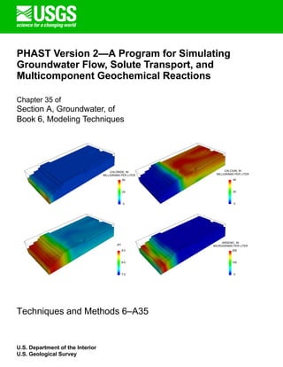
  • 2. COVER ILLUSTRATION: Results of PHAST simulation of the evolution of water chemistry in the Central Oklahoma aquifer (example 4 of this report). Clockwise from upper left are the distribution of chloride concentrations, calcium concentrations, arsenic concentrations, and pH after 1,000,000 years of simulated groundwater flow and reaction. View is from the southwest looking to the northeast. 100 0 CHLORIDE, IN MILLIGRAMS PER LITER CALCIUM, IN MILLIGRAMS PER LITER ARSENIC, IN MICROGRAMS PER LITER pH 8.0 7.0 9.0 20 0 40 25 0 50 200
  • 3. PHAST Version 2—A Program for Simulating Groundwater Flow, Solute Transport, and Multicomponent Geochemical Reactions By David L. Parkhurst, Kenneth L. Kipp, and Scott R. Charlton Chapter 35 of Section A, Groundwater, of Book 6, Modeling Techniques U.S. Department of the Interior U.S. Geological Survey Techniques and Methods 6–A35
  • 4. U.S. Department of the Interior KEN SALAZAR, Secretary U.S. Geological Survey Marcia K. McNutt, Director U.S. Geological Survey, Denver, Colorado: 2010 This and other USGS information products are available at http://store.usgs.gov/ U.S. Geological Survey Box 25286, Denver Federal Center Denver, CO 80225 To learn about the USGS and its information products visit http://www.usgs.gov/ 1-888-ASK-USGS Any use of trade, product, or firm names in this publication is for descriptive purposes only and does not imply endorsement by the U.S. Government. Although this report is in the public domain, permission must be secured from the individual copyright owners to reproduce any copyrighted materials contained within this report. Suggested citation: Parkhurst, D.L., Kipp, K.L., and Charlton, S.R., 2010, PHAST Version 2—A program for simulating groundwater flow, solute transport, and multicomponent geochemical reactions: U.S. Geological Survey Techniques and Methods 6–A35, 235 p.
  • 5. iii Contents Abstract . . . . . . . . . . . . . . . . . . . . . . . . . . . . . . . . . . . . . . . . . . . . . . . . . . . . . . . . . . . . . . . . . 1 Chapter 1. Introduction . . . . . . . . . . . . . . . . . . . . . . . . . . . . . . . . . . . . . . . . . . . . . . . . . . . . . 5 1.1. Enhancements in PHAST Version 2 . . . . . . . . . . . . . . . . . . . . . . . . . . . . . . . . . . . . 5 1.2. Applicability . . . . . . . . . . . . . . . . . . . . . . . . . . . . . . . . . . . . . . . . . . . . . . . . . . . . . . . 6 1.3. Simulator Capabilities . . . . . . . . . . . . . . . . . . . . . . . . . . . . . . . . . . . . . . . . . . . . . . . 7 1.4. Simulator Results . . . . . . . . . . . . . . . . . . . . . . . . . . . . . . . . . . . . . . . . . . . . . . . . . . 7 1.5. Numerical Implementation. . . . . . . . . . . . . . . . . . . . . . . . . . . . . . . . . . . . . . . . . . . . 8 1.6. Computer Resources . . . . . . . . . . . . . . . . . . . . . . . . . . . . . . . . . . . . . . . . . . . . . . . 8 1.7. Purpose and Scope. . . . . . . . . . . . . . . . . . . . . . . . . . . . . . . . . . . . . . . . . . . . . . . . . 9 Chapter 2. Running the Simulator . . . . . . . . . . . . . . . . . . . . . . . . . . . . . . . . . . . . . . . . . . . . 11 2.1. Input Files . . . . . . . . . . . . . . . . . . . . . . . . . . . . . . . . . . . . . . . . . . . . . . . . . . . . . . . .11 2.2. Output Files. . . . . . . . . . . . . . . . . . . . . . . . . . . . . . . . . . . . . . . . . . . . . . . . . . . . . . .11 2.3. Program Execution . . . . . . . . . . . . . . . . . . . . . . . . . . . . . . . . . . . . . . . . . . . . . . . . 13 Chapter 3. Thermodynamic Database and Chemistry Data Files . . . . . . . . . . . . . . . . . . . . 15 3.1. Thermodynamic Database File . . . . . . . . . . . . . . . . . . . . . . . . . . . . . . . . . . . . . . . 15 3.2. Chemistry Data File. . . . . . . . . . . . . . . . . . . . . . . . . . . . . . . . . . . . . . . . . . . . . . . . 16 3.2.1. Chemical Initial and Boundary Conditions for Reactive Transport. . . . . . . . 16 3.2.2. Output of Chemical Data . . . . . . . . . . . . . . . . . . . . . . . . . . . . . . . . . . . . . . . 20 Chapter 4. Flow and Transport Data File . . . . . . . . . . . . . . . . . . . . . . . . . . . . . . . . . . . . . . 21 4.1. Organization of the Flow and Transport Data File. . . . . . . . . . . . . . . . . . . . . . . . . 21 4.2. Spatial Data. . . . . . . . . . . . . . . . . . . . . . . . . . . . . . . . . . . . . . . . . . . . . . . . . . . . . . 23 4.2.1. Zones . . . . . . . . . . . . . . . . . . . . . . . . . . . . . . . . . . . . . . . . . . . . . . . . . . . . . . 24 4.2.1.1. Domain . . . . . . . . . . . . . . . . . . . . . . . . . . . . . . . . . . . . . . . . . . . . . . . . 25 4.2.1.2. Boxes . . . . . . . . . . . . . . . . . . . . . . . . . . . . . . . . . . . . . . . . . . . . . . . . . 25 4.2.1.3. Wedges. . . . . . . . . . . . . . . . . . . . . . . . . . . . . . . . . . . . . . . . . . . . . . . . 25 4.2.1.4. Prisms. . . . . . . . . . . . . . . . . . . . . . . . . . . . . . . . . . . . . . . . . . . . . . . . . 25 4.2.1.5. Use of Zones for Defining Porous-Media Properties . . . . . . . . . . . . . 27 4.2.1.6. Use of Zones for Defining Initial- and Boundary-Condition Properties 28 4.2.1.7. Property Definitions . . . . . . . . . . . . . . . . . . . . . . . . . . . . . . . . . . . . . . 29 4.2.2. Rivers, Drains, and Wells. . . . . . . . . . . . . . . . . . . . . . . . . . . . . . . . . . . . . . . 29 4.2.3. One-, Two-, and Three-Dimensional Interpolation. . . . . . . . . . . . . . . . . . . . 30 4.3. Transient Data. . . . . . . . . . . . . . . . . . . . . . . . . . . . . . . . . . . . . . . . . . . . . . . . . . . . 31 4.4. Documentation Conventions . . . . . . . . . . . . . . . . . . . . . . . . . . . . . . . . . . . . . . . . . 31 4.5. Description of Input for Zones . . . . . . . . . . . . . . . . . . . . . . . . . . . . . . . . . . . . . . . . 33 Example . . . . . . . . . . . . . . . . . . . . . . . . . . . . . . . . . . . . . . . . . . . . . . . . . . . . . . . . . 33 Explanation . . . . . . . . . . . . . . . . . . . . . . . . . . . . . . . . . . . . . . . . . . . . . . . . . . . . . . 34 Notes . . . . . . . . . . . . . . . . . . . . . . . . . . . . . . . . . . . . . . . . . . . . . . . . . . . . . . . . . . . 36 Example Problems. . . . . . . . . . . . . . . . . . . . . . . . . . . . . . . . . . . . . . . . . . . . . . . . . 37 4.6. Description of Input for Properties. . . . . . . . . . . . . . . . . . . . . . . . . . . . . . . . . . . . . 37 Example 1 . . . . . . . . . . . . . . . . . . . . . . . . . . . . . . . . . . . . . . . . . . . . . . . . . . . . . . . 38
  • 6. iv Explanation 1 . . . . . . . . . . . . . . . . . . . . . . . . . . . . . . . . . . . . . . . . . . . . . . . . . . . . . 38 Notes 1 . . . . . . . . . . . . . . . . . . . . . . . . . . . . . . . . . . . . . . . . . . . . . . . . . . . . . . . . . . 40 Example 2 . . . . . . . . . . . . . . . . . . . . . . . . . . . . . . . . . . . . . . . . . . . . . . . . . . . . . . . . 41 Explanation 2 . . . . . . . . . . . . . . . . . . . . . . . . . . . . . . . . . . . . . . . . . . . . . . . . . . . . . 42 Notes 2 . . . . . . . . . . . . . . . . . . . . . . . . . . . . . . . . . . . . . . . . . . . . . . . . . . . . . . . . . . 43 Example Problems . . . . . . . . . . . . . . . . . . . . . . . . . . . . . . . . . . . . . . . . . . . . . . . . . 43 4.7. Description of Keyword Data Blocks . . . . . . . . . . . . . . . . . . . . . . . . . . . . . . . . . . . 44 CHEMISTRY_IC . . . . . . . . . . . . . . . . . . . . . . . . . . . . . . . . . . . . . . . . . . . . . . . . . . . 45 Example . . . . . . . . . . . . . . . . . . . . . . . . . . . . . . . . . . . . . . . . . . . . . . . . . . . . . . 45 Explanation . . . . . . . . . . . . . . . . . . . . . . . . . . . . . . . . . . . . . . . . . . . . . . . . . . . . 45 Notes . . . . . . . . . . . . . . . . . . . . . . . . . . . . . . . . . . . . . . . . . . . . . . . . . . . . . . . . 48 Example Problems . . . . . . . . . . . . . . . . . . . . . . . . . . . . . . . . . . . . . . . . . . . . . . 49 DRAIN. . . . . . . . . . . . . . . . . . . . . . . . . . . . . . . . . . . . . . . . . . . . . . . . . . . . . . . . . . . 50 Example . . . . . . . . . . . . . . . . . . . . . . . . . . . . . . . . . . . . . . . . . . . . . . . . . . . . . . 50 Explanation . . . . . . . . . . . . . . . . . . . . . . . . . . . . . . . . . . . . . . . . . . . . . . . . . . . . 50 Notes . . . . . . . . . . . . . . . . . . . . . . . . . . . . . . . . . . . . . . . . . . . . . . . . . . . . . . . . 51 Example Problems . . . . . . . . . . . . . . . . . . . . . . . . . . . . . . . . . . . . . . . . . . . . . . 52 END. . . . . . . . . . . . . . . . . . . . . . . . . . . . . . . . . . . . . . . . . . . . . . . . . . . . . . . . . . . . . 53 Example Problems . . . . . . . . . . . . . . . . . . . . . . . . . . . . . . . . . . . . . . . . . . . . . . 53 FLUX_BC . . . . . . . . . . . . . . . . . . . . . . . . . . . . . . . . . . . . . . . . . . . . . . . . . . . . . . . . 54 Example . . . . . . . . . . . . . . . . . . . . . . . . . . . . . . . . . . . . . . . . . . . . . . . . . . . . . . 54 Explanation . . . . . . . . . . . . . . . . . . . . . . . . . . . . . . . . . . . . . . . . . . . . . . . . . . . . 54 Notes . . . . . . . . . . . . . . . . . . . . . . . . . . . . . . . . . . . . . . . . . . . . . . . . . . . . . . . . 55 Example Problems . . . . . . . . . . . . . . . . . . . . . . . . . . . . . . . . . . . . . . . . . . . . . . 56 FREE_SURFACE_BC . . . . . . . . . . . . . . . . . . . . . . . . . . . . . . . . . . . . . . . . . . . . . . 57 Example . . . . . . . . . . . . . . . . . . . . . . . . . . . . . . . . . . . . . . . . . . . . . . . . . . . . . . 57 Explanation . . . . . . . . . . . . . . . . . . . . . . . . . . . . . . . . . . . . . . . . . . . . . . . . . . . . 57 Notes . . . . . . . . . . . . . . . . . . . . . . . . . . . . . . . . . . . . . . . . . . . . . . . . . . . . . . . . 57 Example Problems . . . . . . . . . . . . . . . . . . . . . . . . . . . . . . . . . . . . . . . . . . . . . . 57 GRID . . . . . . . . . . . . . . . . . . . . . . . . . . . . . . . . . . . . . . . . . . . . . . . . . . . . . . . . . . . . 58 Example . . . . . . . . . . . . . . . . . . . . . . . . . . . . . . . . . . . . . . . . . . . . . . . . . . . . . . 58 Example . . . . . . . . . . . . . . . . . . . . . . . . . . . . . . . . . . . . . . . . . . . . . . . . . . . . . . 58 Notes . . . . . . . . . . . . . . . . . . . . . . . . . . . . . . . . . . . . . . . . . . . . . . . . . . . . . . . . 61 Example Problems . . . . . . . . . . . . . . . . . . . . . . . . . . . . . . . . . . . . . . . . . . . . . . 62 HEAD_IC . . . . . . . . . . . . . . . . . . . . . . . . . . . . . . . . . . . . . . . . . . . . . . . . . . . . . . . . 63 Example 1. . . . . . . . . . . . . . . . . . . . . . . . . . . . . . . . . . . . . . . . . . . . . . . . . . . . . 63 Explanation 1 . . . . . . . . . . . . . . . . . . . . . . . . . . . . . . . . . . . . . . . . . . . . . . . . . . 63 Example 2. . . . . . . . . . . . . . . . . . . . . . . . . . . . . . . . . . . . . . . . . . . . . . . . . . . . . 63 Explanation 2 . . . . . . . . . . . . . . . . . . . . . . . . . . . . . . . . . . . . . . . . . . . . . . . . . . 63 Notes . . . . . . . . . . . . . . . . . . . . . . . . . . . . . . . . . . . . . . . . . . . . . . . . . . . . . . . . 64 Example Problems . . . . . . . . . . . . . . . . . . . . . . . . . . . . . . . . . . . . . . . . . . . . . . 64 LEAKY_BC. . . . . . . . . . . . . . . . . . . . . . . . . . . . . . . . . . . . . . . . . . . . . . . . . . . . . . . 65 Example . . . . . . . . . . . . . . . . . . . . . . . . . . . . . . . . . . . . . . . . . . . . . . . . . . . . . . 65
  • 7. v Explanation . . . . . . . . . . . . . . . . . . . . . . . . . . . . . . . . . . . . . . . . . . . . . . . . . . . 65 Notes . . . . . . . . . . . . . . . . . . . . . . . . . . . . . . . . . . . . . . . . . . . . . . . . . . . . . . . . 67 Example Problems. . . . . . . . . . . . . . . . . . . . . . . . . . . . . . . . . . . . . . . . . . . . . . 68 MEDIA . . . . . . . . . . . . . . . . . . . . . . . . . . . . . . . . . . . . . . . . . . . . . . . . . . . . . . . . . . 69 Example. . . . . . . . . . . . . . . . . . . . . . . . . . . . . . . . . . . . . . . . . . . . . . . . . . . . . . 69 Explanation . . . . . . . . . . . . . . . . . . . . . . . . . . . . . . . . . . . . . . . . . . . . . . . . . . . 69 Notes . . . . . . . . . . . . . . . . . . . . . . . . . . . . . . . . . . . . . . . . . . . . . . . . . . . . . . . . 71 Example Problems. . . . . . . . . . . . . . . . . . . . . . . . . . . . . . . . . . . . . . . . . . . . . . 73 PRINT_FREQUENCY . . . . . . . . . . . . . . . . . . . . . . . . . . . . . . . . . . . . . . . . . . . . . . 74 Example. . . . . . . . . . . . . . . . . . . . . . . . . . . . . . . . . . . . . . . . . . . . . . . . . . . . . . 74 Explanation . . . . . . . . . . . . . . . . . . . . . . . . . . . . . . . . . . . . . . . . . . . . . . . . . . . 74 Notes . . . . . . . . . . . . . . . . . . . . . . . . . . . . . . . . . . . . . . . . . . . . . . . . . . . . . . . . 80 Example Problems. . . . . . . . . . . . . . . . . . . . . . . . . . . . . . . . . . . . . . . . . . . . . . 81 PRINT_INITIAL . . . . . . . . . . . . . . . . . . . . . . . . . . . . . . . . . . . . . . . . . . . . . . . . . . . 82 Example. . . . . . . . . . . . . . . . . . . . . . . . . . . . . . . . . . . . . . . . . . . . . . . . . . . . . . 82 Explanation . . . . . . . . . . . . . . . . . . . . . . . . . . . . . . . . . . . . . . . . . . . . . . . . . . . 82 Notes . . . . . . . . . . . . . . . . . . . . . . . . . . . . . . . . . . . . . . . . . . . . . . . . . . . . . . . . 86 Example Problems. . . . . . . . . . . . . . . . . . . . . . . . . . . . . . . . . . . . . . . . . . . . . . 86 PRINT_LOCATIONS . . . . . . . . . . . . . . . . . . . . . . . . . . . . . . . . . . . . . . . . . . . . . . . 87 Example. . . . . . . . . . . . . . . . . . . . . . . . . . . . . . . . . . . . . . . . . . . . . . . . . . . . . . 87 Explanation . . . . . . . . . . . . . . . . . . . . . . . . . . . . . . . . . . . . . . . . . . . . . . . . . . . 87 Notes . . . . . . . . . . . . . . . . . . . . . . . . . . . . . . . . . . . . . . . . . . . . . . . . . . . . . . . . 88 Example Problems. . . . . . . . . . . . . . . . . . . . . . . . . . . . . . . . . . . . . . . . . . . . . . 88 RIVER . . . . . . . . . . . . . . . . . . . . . . . . . . . . . . . . . . . . . . . . . . . . . . . . . . . . . . . . . . 89 Example. . . . . . . . . . . . . . . . . . . . . . . . . . . . . . . . . . . . . . . . . . . . . . . . . . . . . . 89 Explanation . . . . . . . . . . . . . . . . . . . . . . . . . . . . . . . . . . . . . . . . . . . . . . . . . . . 89 Notes . . . . . . . . . . . . . . . . . . . . . . . . . . . . . . . . . . . . . . . . . . . . . . . . . . . . . . . . 91 Example Problems. . . . . . . . . . . . . . . . . . . . . . . . . . . . . . . . . . . . . . . . . . . . . . 93 SOLUTE_TRANSPORT . . . . . . . . . . . . . . . . . . . . . . . . . . . . . . . . . . . . . . . . . . . . 94 Example. . . . . . . . . . . . . . . . . . . . . . . . . . . . . . . . . . . . . . . . . . . . . . . . . . . . . . 94 Explanation . . . . . . . . . . . . . . . . . . . . . . . . . . . . . . . . . . . . . . . . . . . . . . . . . . . 94 Notes . . . . . . . . . . . . . . . . . . . . . . . . . . . . . . . . . . . . . . . . . . . . . . . . . . . . . . . . 94 Example Problems. . . . . . . . . . . . . . . . . . . . . . . . . . . . . . . . . . . . . . . . . . . . . . 94 SOLUTION_METHOD. . . . . . . . . . . . . . . . . . . . . . . . . . . . . . . . . . . . . . . . . . . . . . 95 Example 1 . . . . . . . . . . . . . . . . . . . . . . . . . . . . . . . . . . . . . . . . . . . . . . . . . . . . 95 Explanation 1. . . . . . . . . . . . . . . . . . . . . . . . . . . . . . . . . . . . . . . . . . . . . . . . . . 95 Notes 1 . . . . . . . . . . . . . . . . . . . . . . . . . . . . . . . . . . . . . . . . . . . . . . . . . . . . . . 97 Example 2 . . . . . . . . . . . . . . . . . . . . . . . . . . . . . . . . . . . . . . . . . . . . . . . . . . . . 98 Explanation 2. . . . . . . . . . . . . . . . . . . . . . . . . . . . . . . . . . . . . . . . . . . . . . . . . . 98 Notes 2 . . . . . . . . . . . . . . . . . . . . . . . . . . . . . . . . . . . . . . . . . . . . . . . . . . . . . . 99 Example Problems. . . . . . . . . . . . . . . . . . . . . . . . . . . . . . . . . . . . . . . . . . . . . . 99 SPECIFIED_HEAD_BC. . . . . . . . . . . . . . . . . . . . . . . . . . . . . . . . . . . . . . . . . . . . 100 Example. . . . . . . . . . . . . . . . . . . . . . . . . . . . . . . . . . . . . . . . . . . . . . . . . . . . . 100
  • 8. vi Explanation . . . . . . . . . . . . . . . . . . . . . . . . . . . . . . . . . . . . . . . . . . . . . . . . . . . 100 Notes . . . . . . . . . . . . . . . . . . . . . . . . . . . . . . . . . . . . . . . . . . . . . . . . . . . . . . . 102 Example Problems . . . . . . . . . . . . . . . . . . . . . . . . . . . . . . . . . . . . . . . . . . . . . 102 STEADY_FLOW. . . . . . . . . . . . . . . . . . . . . . . . . . . . . . . . . . . . . . . . . . . . . . . . . . 103 Example . . . . . . . . . . . . . . . . . . . . . . . . . . . . . . . . . . . . . . . . . . . . . . . . . . . . . 103 Explanation . . . . . . . . . . . . . . . . . . . . . . . . . . . . . . . . . . . . . . . . . . . . . . . . . . . 103 Notes . . . . . . . . . . . . . . . . . . . . . . . . . . . . . . . . . . . . . . . . . . . . . . . . . . . . . . . 104 Example Problems . . . . . . . . . . . . . . . . . . . . . . . . . . . . . . . . . . . . . . . . . . . . . 105 TIME_CONTROL . . . . . . . . . . . . . . . . . . . . . . . . . . . . . . . . . . . . . . . . . . . . . . . . . 106 Example . . . . . . . . . . . . . . . . . . . . . . . . . . . . . . . . . . . . . . . . . . . . . . . . . . . . . 106 Explanation . . . . . . . . . . . . . . . . . . . . . . . . . . . . . . . . . . . . . . . . . . . . . . . . . . . 106 Notes . . . . . . . . . . . . . . . . . . . . . . . . . . . . . . . . . . . . . . . . . . . . . . . . . . . . . . . 107 Example Problems . . . . . . . . . . . . . . . . . . . . . . . . . . . . . . . . . . . . . . . . . . . . . 108 TITLE . . . . . . . . . . . . . . . . . . . . . . . . . . . . . . . . . . . . . . . . . . . . . . . . . . . . . . . . . . 109 Example . . . . . . . . . . . . . . . . . . . . . . . . . . . . . . . . . . . . . . . . . . . . . . . . . . . . . 109 Explanation . . . . . . . . . . . . . . . . . . . . . . . . . . . . . . . . . . . . . . . . . . . . . . . . . . . 109 Notes . . . . . . . . . . . . . . . . . . . . . . . . . . . . . . . . . . . . . . . . . . . . . . . . . . . . . . . 109 Example Problems . . . . . . . . . . . . . . . . . . . . . . . . . . . . . . . . . . . . . . . . . . . . . 109 UNITS . . . . . . . . . . . . . . . . . . . . . . . . . . . . . . . . . . . . . . . . . . . . . . . . . . . . . . . . . . 110 Example . . . . . . . . . . . . . . . . . . . . . . . . . . . . . . . . . . . . . . . . . . . . . . . . . . . . . 110 Explanation . . . . . . . . . . . . . . . . . . . . . . . . . . . . . . . . . . . . . . . . . . . . . . . . . . . 110 Notes . . . . . . . . . . . . . . . . . . . . . . . . . . . . . . . . . . . . . . . . . . . . . . . . . . . . . . . 114 Example Problems . . . . . . . . . . . . . . . . . . . . . . . . . . . . . . . . . . . . . . . . . . . . . 115 WELL . . . . . . . . . . . . . . . . . . . . . . . . . . . . . . . . . . . . . . . . . . . . . . . . . . . . . . . . . . 116 Example . . . . . . . . . . . . . . . . . . . . . . . . . . . . . . . . . . . . . . . . . . . . . . . . . . . . . 116 Explanation . . . . . . . . . . . . . . . . . . . . . . . . . . . . . . . . . . . . . . . . . . . . . . . . . . . 116 Notes . . . . . . . . . . . . . . . . . . . . . . . . . . . . . . . . . . . . . . . . . . . . . . . . . . . . . . . 119 Example Problems . . . . . . . . . . . . . . . . . . . . . . . . . . . . . . . . . . . . . . . . . . . . . 120 ZONE_FLOW . . . . . . . . . . . . . . . . . . . . . . . . . . . . . . . . . . . . . . . . . . . . . . . . . . . . 121 Example . . . . . . . . . . . . . . . . . . . . . . . . . . . . . . . . . . . . . . . . . . . . . . . . . . . . . 121 Explanation . . . . . . . . . . . . . . . . . . . . . . . . . . . . . . . . . . . . . . . . . . . . . . . . . . . 121 Notes . . . . . . . . . . . . . . . . . . . . . . . . . . . . . . . . . . . . . . . . . . . . . . . . . . . . . . . 122 Example Problems . . . . . . . . . . . . . . . . . . . . . . . . . . . . . . . . . . . . . . . . . . . . . 122 Chapter 5. Output Files . . . . . . . . . . . . . . . . . . . . . . . . . . . . . . . . . . . . . . . . . . . . . . . . . . . 123 5.1. Content of Output Files . . . . . . . . . . . . . . . . . . . . . . . . . . . . . . . . . . . . . . . . . . . . 123 5.2. Selection of Data for Chemical Output Files . . . . . . . . . . . . . . . . . . . . . . . . . . . . 128 5.3. Output Files for Postprocessing . . . . . . . . . . . . . . . . . . . . . . . . . . . . . . . . . . . . . . 129 5.4. Diagnostic Output Files . . . . . . . . . . . . . . . . . . . . . . . . . . . . . . . . . . . . . . . . . . . . 129 Chapter 6. Examples . . . . . . . . . . . . . . . . . . . . . . . . . . . . . . . . . . . . . . . . . . . . . . . . . . . . . 131 6.1. Verification Examples. . . . . . . . . . . . . . . . . . . . . . . . . . . . . . . . . . . . . . . . . . . . . . 131 6.2. Example 1: Pulse Source of Chemical Constituent that Undergoes Sorption and Decay . . . . . . . . . . . . . . . . . . . . . . . . . . . . . . . . . . . . . . . . . . . . . . . . . . . . . . . . . . 132 6.3. Example 2: Chain of Four Kinetically Decaying Reactants . . . . . . . . . . . . . . . . . 139
  • 9. vii 6.4. Example 3: Aerobic Consumption of a Substrate with Biomass Growth. . . . . . . 144 6.5. Example 4: Regional-Scale Transport and Reactions in the Central Oklahoma Aquifer . . . . . . . . . . . . . . . . . . . . . . . . . . . . . . . . . . . . . . . . . . . . . . . . 150 6.5.1. Initial Conditions. . . . . . . . . . . . . . . . . . . . . . . . . . . . . . . . . . . . . . . . . . . . . 152 6.5.2. Chemistry Data File . . . . . . . . . . . . . . . . . . . . . . . . . . . . . . . . . . . . . . . . . . 153 6.5.3. Flow and Transport Data File. . . . . . . . . . . . . . . . . . . . . . . . . . . . . . . . . . . 155 6.5.4. Simulation Results . . . . . . . . . . . . . . . . . . . . . . . . . . . . . . . . . . . . . . . . . . . 160 6.6. Example 5: Simulation of Groundwater Flow for a Sewage Wastewater Plume at Cape Cod, Massachusetts. . . . . . . . . . . . . . . . . . . . . . . . . . . . . . . . . . . . . . . . . . 161 6.6.1. Flow and Transport Data File. . . . . . . . . . . . . . . . . . . . . . . . . . . . . . . . . . . 163 6.6.2. Steady-Flow Simulation Results . . . . . . . . . . . . . . . . . . . . . . . . . . . . . . . . 171 6.6.3. Transient Simulation Results . . . . . . . . . . . . . . . . . . . . . . . . . . . . . . . . . . . 171 6.7. Example 6: Simulation of Ammonium Transport and Reactions for a Sewage Wastewater Plume at Cape Cod, Massachusetts . . . . . . . . . . . . . . . . . . . . . . . . 172 6.7.1. Chemistry Data File . . . . . . . . . . . . . . . . . . . . . . . . . . . . . . . . . . . . . . . . . . 172 6.7.2. Flow and Transport Data File. . . . . . . . . . . . . . . . . . . . . . . . . . . . . . . . . . . 173 6.7.3. Simulation . . . . . . . . . . . . . . . . . . . . . . . . . . . . . . . . . . . . . . . . . . . . . . . . . 175 6.7.3.1. Accuracy of the Transport Solution. . . . . . . . . . . . . . . . . . . . . . . . . . 175 6.7.3.2. Simulation Results . . . . . . . . . . . . . . . . . . . . . . . . . . . . . . . . . . . . . . 181 Chapter 7. Notation . . . . . . . . . . . . . . . . . . . . . . . . . . . . . . . . . . . . . . . . . . . . . . . . . . . . . . 183 7.1. Roman Characters . . . . . . . . . . . . . . . . . . . . . . . . . . . . . . . . . . . . . . . . . . . . . . . 183 7.2. Greek Characters . . . . . . . . . . . . . . . . . . . . . . . . . . . . . . . . . . . . . . . . . . . . . . . . 186 7.3. Mathematical Operators and Special Functions . . . . . . . . . . . . . . . . . . . . . . . . . 187 References Cited. . . . . . . . . . . . . . . . . . . . . . . . . . . . . . . . . . . . . . . . . . . . . . . . . . . . . . . . 189 Appendix A. Three-Dimensional Visualization of PHAST Simulation Results. . . . . . . . . . 193 Appendix B. Using PHASTHDF to Extract Data from the HDF Output File . . . . . . . . . . . 195 Appendix C. Parallel-Processing Version of PHAST. . . . . . . . . . . . . . . . . . . . . . . . . . . . . 197 C.1. Parallelization of PHAST . . . . . . . . . . . . . . . . . . . . . . . . . . . . . . . . . . . . . . . . . . 197 C.2. Running the Parallel Version . . . . . . . . . . . . . . . . . . . . . . . . . . . . . . . . . . . . . . . 201 Appendix D. Theory and Numerical Implementation. . . . . . . . . . . . . . . . . . . . . . . . . . . . . 203 D.1. Flow and Transport Equations . . . . . . . . . . . . . . . . . . . . . . . . . . . . . . . . . . . . . . 203 D.1.1. Components . . . . . . . . . . . . . . . . . . . . . . . . . . . . . . . . . . . . . . . . . . . . . . . 205 D.1.2. Spatial Discretization. . . . . . . . . . . . . . . . . . . . . . . . . . . . . . . . . . . . . . . . . 206 D.1.3. Temporal Discretization. . . . . . . . . . . . . . . . . . . . . . . . . . . . . . . . . . . . . . . 208 D.1.4. Automatic Time-Step Algorithm for Steady-State Flow Simulation . . . . . . 210 D.2. Chemical-Reaction Equations . . . . . . . . . . . . . . . . . . . . . . . . . . . . . . . . . . . . . . 210 D.2.1. Equilibrium Reactions . . . . . . . . . . . . . . . . . . . . . . . . . . . . . . . . . . . . . . . . 210 D.2.2. Component Mole Balance . . . . . . . . . . . . . . . . . . . . . . . . . . . . . . . . . . . . . 211 D.2.3. Kinetic Reactions. . . . . . . . . . . . . . . . . . . . . . . . . . . . . . . . . . . . . . . . . . . . 211 D.3. Property Functions and Transport Coefficients. . . . . . . . . . . . . . . . . . . . . . . . . . .211 D.4. Well-Source Conditions . . . . . . . . . . . . . . . . . . . . . . . . . . . . . . . . . . . . . . . . . . . 213 D.5. Boundary Conditions . . . . . . . . . . . . . . . . . . . . . . . . . . . . . . . . . . . . . . . . . . . . . 215 D.5.1. Specified-Head Boundary with Associated-Solution Composition . . . . . . 215
  • 10. viii D.5.2. Specified-Head Boundary with Specified-Solution Composition . . . . . . . . 216 D.5.3. Flux Boundary . . . . . . . . . . . . . . . . . . . . . . . . . . . . . . . . . . . . . . . . . . . . . . 216 D.5.4. Leaky Boundary . . . . . . . . . . . . . . . . . . . . . . . . . . . . . . . . . . . . . . . . . . . . . 217 D.5.5. River Boundary. . . . . . . . . . . . . . . . . . . . . . . . . . . . . . . . . . . . . . . . . . . . . . 218 D.5.6. Drain Boundaries . . . . . . . . . . . . . . . . . . . . . . . . . . . . . . . . . . . . . . . . . . . . 222 D.5.7. Free-Surface Boundary . . . . . . . . . . . . . . . . . . . . . . . . . . . . . . . . . . . . . . . 223 D.5.8. Boundary-Condition Compatibility . . . . . . . . . . . . . . . . . . . . . . . . . . . . . . . 225 D.6. Initial Conditions . . . . . . . . . . . . . . . . . . . . . . . . . . . . . . . . . . . . . . . . . . . . . . . . . 226 D.7. Method of Solution. . . . . . . . . . . . . . . . . . . . . . . . . . . . . . . . . . . . . . . . . . . . . . . . 228 D.7.1. Operator Splitting and Sequential Solution. . . . . . . . . . . . . . . . . . . . . . . . . 228 D.7.2. Linear-Equation Solvers for Flow and Transport Finite-Difference Equations . . . . . . . . . . . . . . . . . . . . . . . . . . . . . . . . . . . . . . . . . . . . . . . . . . 230 D.7.3. Solving Equilibrium and Kinetic Chemical Equations . . . . . . . . . . . . . . . . . 232 D.8. Accuracy from Spatial and Temporal Discretization. . . . . . . . . . . . . . . . . . . . . . . 232 D.9. Global Mass-Balance Calculations . . . . . . . . . . . . . . . . . . . . . . . . . . . . . . . . . . . 233 D.10. Zone Flow-Rate Calculation . . . . . . . . . . . . . . . . . . . . . . . . . . . . . . . . . . . . . . . 234 D.11. Nodal Velocity Calculation . . . . . . . . . . . . . . . . . . . . . . . . . . . . . . . . . . . . . . . . . 235 Figures 2.1. Figure showing the relation between input and output files and the execution of the two programs PHASTINPUT and PHAST . . . . . . . . . . . . . . . . . . . . . . . . . . . . . 14 4.1.–4.9. Figures showing: 4.1. The grid region, boundary nodes, and one shaded element. . . . . . . . . . . . . . . 23 4.2. The grid region, boundary of the active grid region, boundary nodes, cell boundaries, and one shaded cell . . . . . . . . . . . . . . . . . . . . . . . . . . . . . . . . . . . 24 4.3. Identifying numbers for four wedges with axis of right angle parallel to the Y axis . . . . . . . . . . . . . . . . . . . . . . . . . . . . . . . . . . . . . . . . . . . . . . . . . . . . . . . . 25 4.4. Prism defined by rectangular perimeter, default top, and bottom defined by an ArcInfo ASCII raster file with elevation of impermeable bedrock . . . . . . . . . . . 26 4.5. Rectangular box used to select elements from a two-dimensional grid, and the elements selected by the box . . . . . . . . . . . . . . . . . . . . . . . . . . . . . . . . . . . . . . 27 4.6. The parts of eight elements contained within a cell and the parts of four elements located within each cell face . . . . . . . . . . . . . . . . . . . . . . . . . . . . . . . 27 4.7. Rectangular zone used for determining areas of application for leaky and flux boundary conditions or to select nodes for initial conditions and specified- head boundary conditions, and the nodes and cells selected by the zone . . . . . . 4.8. Flow-control diagram for parallel-processing version of PHAST. . . . . . . . . . . . 72 4.9. Discretization of river segments for a river and its tributary . . . . . . . . . . . . . . . 92 6.1.–6.3. Figures showing: 6.1. Example 1, analytical solution for concentration at 120 seconds of a pulse of solute that undergoes linear sorption and linear decay compared to numerical solutions . . . . . . . . . . . . . . . . . . . . . . . . . . . . . . . . . . . . . . . . . . . . . 138 6.2. Example 2, analytical solution compared to simulation results for concentra- tions at 400 days and Z=12.5 meters of a chain of decay products . . . . . . . . 143
  • 11. ix 6.3. Example 3, concentrations of substrate, biomass, and dissolved oxygen at 37 days. . . . . . . . . . . . . . . . . . . . . . . . . . . . . . . . . . . . . . . . . . . . . . . . . . . . . . 150 6.4. Map showing locations in the Central Oklahoma aquifer with arsenic concentra- tions greater than 50 micrograms per liter and PHAST model area . . . . . . . . . . . 151 6.5.–6.6. Figures showing: 6.5. Example 4, locations of boundary conditions and steady-state head distribution . . . . . . . . . . . . . . . . . . . . . . . . . . . . . . . . . . . . . . . . . . . . . . . . . . . 159 6.6. Example 4, distribution of chloride concentrations, calcium concentrations, pH, and arsenic concentrations after 1,000,000-year simulation of the evolu- tion of water in the Central Oklahoma aquifer . . . . . . . . . . . . . . . . . . . . . . . . 160 6.7. Example 5, map showing wastewater infiltration beds and selected surface-water features of Cape Cod, Massachusetts. . . . . . . . . . . . . . . . . . . . . . . . . . . . . . . . . . 162 6.8.–6.13. Figures showing: 6.8. Example 5, zones used to define the media properties and active area of the model domain. . . . . . . . . . . . . . . . . . . . . . . . . . . . . . . . . . . . . . . . . . . . . . . . . 168 6.9. Example 5, boundary-condition definitions. . . . . . . . . . . . . . . . . . . . . . . . . . . 169 6.10. Example 5, grid and boundary conditions for the transient simulation. . . . . 170 6.11. Example 5, steady-flow head distribution. . . . . . . . . . . . . . . . . . . . . . . . . . . 171 6.12. Example 6, distribution of ammonium and nitrate after year 1995. . . . . . . . 180 6.13. Example 6, input of nitrogen through the infiltration beds and simulated discharge of nitrogen to Ashumet Pond and rivers and ocean . . . . . . . . . . . 181 B.1.–B.3. PHASTHDF input screen: B.1. For selection of HDF output file from which data are to be extracted . . . . . . 195 B.2. Associated with the first (X-Coor) and fourth (Scalars) of five tabs that allow selection of model nodes and chemical data to be extracted from the HDF output file . . . . . . . . . . . . . . . . . . . . . . . . . . . . . . . . . . . . . . . . . . . . . . . . . . . . 196 B.3. Used to specify the file name for the export file . . . . . . . . . . . . . . . . . . . . . . . 196 C.1. Flow-control diagram for parallel-processing version of PHAST . . . . . . . . . . . . . 198 D.1.–D.3. Figures showing: D.1. Grid of node points that covers the model domain. . . . . . . . . . . . . . . . . . . . . 207 D.2. Schematic section showing geometry for a river boundary . . . . . . . . . . . . . . 219 D.3. Steps by which river segments and river segment properties are determined . . . . . . . . . . . . . . . . . . . . . . . . . . . . . . . . . . . . . . . . . . . . . . . . . . . 220 Tables 2.1. List of output files that may be generated by a PHAST simulation. . . . . . . . . . . . 12 3.1. Keyword data blocks commonly used in the thermodynamic database file. . . . . 16 3.2. Elements and element valence states included in default thermodynamic database phast.dat, including PHAST notation and default formulas for gram for- mula weight . . . . . . . . . . . . . . . . . . . . . . . . . . . . . . . . . . . . . . . . . . . . . . . . . . . . . 17 3.3. Keyword data blocks commonly used in the chemistry data file. . . . . . . . . . . . . . 19 4.1. Keyword data blocks for the flow and transport data file.. . . . . . . . . . . . . . . . . . . 22 6.1. Run times for example problems.. . . . . . . . . . . . . . . . . . . . . . . . . . . . . . . . . . . . 131 6.2. Chemical and physical parameters for example 1. . . . . . . . . . . . . . . . . . . . . . . 132 6.3. Chemistry data file for example 1. . . . . . . . . . . . . . . . . . . . . . . . . . . . . . . . . . . . 134
  • 12. x 6.4. Flow and transport data file for example 1. . . . . . . . . . . . . . . . . . . . . . . . . . . . . . 136 6.5. Chemical and physical parameters for example 2. . . . . . . . . . . . . . . . . . . . . . . . 139 6.6. Chemistry data file for example 2.. . . . . . . . . . . . . . . . . . . . . . . . . . . . . . . . . . . . 140 6.7. Flow and transport data file for example 2. . . . . . . . . . . . . . . . . . . . . . . . . . . . . . 142 6.8. Chemical and physical parameters for example 3. . . . . . . . . . . . . . . . . . . . . . . . 145 6.9. Chemistry data file for example 3.. . . . . . . . . . . . . . . . . . . . . . . . . . . . . . . . . . . . 147 6.10. Flow and transport data file for example 3. . . . . . . . . . . . . . . . . . . . . . . . . . . . . . 149 6.11. Chemistry data file for example 4.. . . . . . . . . . . . . . . . . . . . . . . . . . . . . . . . . . . . 154 6.12. Flow and transport data file for example 4. . . . . . . . . . . . . . . . . . . . . . . . . . . . . . 156 6.13. Flow and transport data file for example 5. . . . . . . . . . . . . . . . . . . . . . . . . . . . . . 164 6.14. Chemistry data file for example 6.. . . . . . . . . . . . . . . . . . . . . . . . . . . . . . . . . . . . 173 6.15. Flow and transport data file for example 6. . . . . . . . . . . . . . . . . . . . . . . . . . . . . . 176 D.1. Compatibility among boundary conditions and wells for a cell. . . . . . . . . . . . . . . 226 Conversion Factors SI to Inch/Pound Multiply By To obtain Length centimeter (cm) 0.3937 inch (in.) millimeter (mm) 0.03937 inch (in.) meter (m) 3.281 foot (ft) kilometer (km) 0.6214 mile (mi) meter (m) 1.094 yard (yd) Area square meter (m2 ) 0.0002471 acre square centimeter (cm2 ) 0.001076 square foot (ft2 ) square meter (m2) 10.76 square foot (ft2) Volume liter (L) 1.057 quart (qt) liter (L) 0.2642 gallon (gal) cubic meter (m3 ) 264.2 gallon (gal) cubic meter (m3 ) 0.0002642 million gallons (Mgal) cubic meter (m3) 35.31 cubic foot (ft3) cubic meter (m3 ) 1.308 cubic yard (yd3 )
  • 13. xi Temperature in degrees Celsius (°C) may be converted to degrees Fahrenheit (°F) as follows: °F=(1.8×°C)+32 Temperature in degrees Fahrenheit (°F) may be converted to degrees Celsius (°C) as follows: °C=(°F-32)/1.8 Vertical coordinate information is referenced to the North American Vertical Datum of 1988 (NAVD 88). Horizontal coordinate information is referenced to the North American Datum of 1983 (NAD 83). Altitude, as used in this report, refers to distance above the vertical datum. Flow rate cubic meter per second (m3 /s) 70.07 acre-foot per day (acre-ft/d) cubic meter per year (m3/yr) 0.000811 acre-foot per year (acre-ft/yr) meter per second (m/s) 3.281 foot per second (ft/s) meter per day (m/d) 3.281 foot per day (ft/d) meter per year (m/yr) 3.281 foot per year ft/yr) cubic meter per second (m3 /s) 35.31 cubic foot per second (ft3 /s) cubic meter per second per square kilometer [(m3 /s)/km2 ] 91.49 cubic foot per second per square mile [(ft3 /s)/mi2 ] cubic meter per day (m3 /d) 35.31 cubic foot per day (ft3 /d) Mass gram (g) 0.03527 ounce, avoirdupois (oz) kilogram (kg) 2.205 pound avoirdupois (lb) Pressure kilopascal (kPa) 0.009869 atmosphere, standard (atm) kilopascal (kPa) 0.01 bar Density kilogram per cubic meter (kg/m3) 0.06242 pound per cubic foot (lb/ft3) Energy joule (J) 0.0000002 kilowatthour (kWh) Hydraulic conductivity meter per day (m/d) 3.281 foot per day (ft/d)
  • 14. xii Abbreviations atmosphere atm cubic meter m3 day d equivalent eq gram g gigabytes GB hour hr joule J kilogram kg kilogram of water kgw kilometer km liter L meter m mole mol milliequivalent meq milligram mg millimole mmol microgram μg micromole μmol pascals Pa parts per million ppm second s square meter m2 year yr
  • 15. Abstract 1 Abstract The computer program PHAST (PHREEQC And HST3D) simulates multicomponent, reactive solute transport in three-dimensional saturated groundwater flow systems. PHAST is a versatile groundwater flow and solute-transport simulator with capabilities to model a wide range of equilibrium and kinetic geochem- ical reactions. The flow and transport calculations are based on a modified version of HST3D that is restricted to constant fluid density and constant temperature. The geochemical reactions are simulated with the geochemical model PHREEQC, which is embedded in PHAST. Major enhancements in PHAST Version 2 allow spatial data to be defined in a combination of map and grid coordinate systems, independent of a specific model grid (without node-by-node input). At run time, aquifer properties are interpolated from the spatial data to the model grid; regridding requires only redefinition of the grid without modification of the spatial data. PHAST is applicable to the study of natural and contaminated groundwater systems at a variety of scales ranging from laboratory experiments to local and regional field scales. PHAST can be used in studies of migration of nutrients, inorganic and organic contaminants, and radionuclides; in projects such as aquifer storage and recovery or engineered remediation; and in investigations of the natural rock/water interactions in aquifers. PHAST is not appropriate for unsaturated-zone flow, multiphase flow, or density-dependent flow. A variety of boundary conditions are available in PHAST to simulate flow and transport, including spec- ified-head, flux (specified-flux), and leaky (head-dependent) conditions, as well as the special cases of rivers, drains, and wells. Chemical reactions in PHAST include (1) homogeneous equilibria using an ion-associa- tion or Pitzer specific interaction thermodynamic model; (2) heterogeneous equilibria between the aqueous solution and minerals, ion exchange sites, surface complexation sites, solid solutions, and gases; and (3) kinetic reactions with rates that are a function of solution composition. The aqueous model (elements, chem- ical reactions, and equilibrium constants), minerals, exchangers, surfaces, gases, kinetic reactants, and rate expressions may be defined or modified by the user. A number of options are available to save results of simulations to output files. The data may be saved in three formats: a format suitable for viewing with a text editor; a format suitable for exporting to spread- sheets and postprocessing programs; and in Hierarchical Data Format (HDF), which is a compressed binary format. Data in the HDF file can be visualized on Windows computers with the program Model Viewer and extracted with the utility program PHASTHDF; both programs are distributed with PHAST. Operator splitting of the flow, transport, and geochemical equations is used to separate the three pro- cesses into three sequential calculations. No iterations between transport and reaction calculations are imple- mented. A three-dimensional Cartesian coordinate system and finite-difference techniques are used for the spatial and temporal discretization of the flow and transport equations. The nonlinear chemical equilibrium PHAST Version 2—A Program for Simulating Groundwater Flow, Solute Transport, and Multicomponent Geochemical Reactions By David L. Parkhurst, Kenneth L. Kipp, and Scott R. Charlton
  • 16. 2 PHAST Version 2 equations are solved by a Newton-Raphson method, and the kinetic reaction equations are solved by a Runge-Kutta or an implicit method for integrating ordinary differential equations. The PHAST simulator may require large amounts of memory and long Central Processing Unit (CPU) times. To reduce the long CPU times, a parallel version of PHAST has been developed that runs on a multi- processor computer or on a collection of computers that are networked. The parallel version requires Mes- sage Passing Interface, which is freely available. The parallel version is effective in reducing simulation times. This report documents the use of the PHAST simulator, including running the simulator, preparing the input files, selecting the output files, and visualizing the results. It also presents six examples that verify the numerical method and demonstrate the capabilities of the simulator. PHAST requires three input files. Only the flow and transport file is described in detail in this report. The other two files, the chemistry data file and the database file, are identical to PHREEQC files, and a detailed description of these files is in the PHREEQC documentation. PHAST Version 2 has a number of enhancements to allow simpler definition of spatial information and to avoid grid-dependent (node-by-node) input definitions. Formerly, all spatial data were defined with rect- angular zones. Now wedge-shaped and irregularly shaped volumes may be used to specify the hydrologic and chemical properties of regions within the model domain. Spatial data can be imported from ArcInfo shape and ASCII raster files and from a simple X,Y, Z file format. To accommodate a grid that is not aligned with the coordinate system of the imported files, it is possible to define features in map and grid coordinate systems within the same input file. The definition of leaky and flux boundary conditions has been modified to select only exterior faces within a specified volume of the model domain and to restrict the boundary conditions to the area of defini- tion, which may include fractions of cell faces. Previously, flux and leaky boundary conditions were applied only to entire cell faces; thus, the area could vary as the model grid was refined and cell sizes changed. New capabilities have been added to interpolate spatial data to the two- or three-dimensional locations of cells and elements. Two-dimensional interpolation is used to define surfaces for the tops and bottoms of three-dimensional regions within the model domain. Surfaces are created by two-dimensional interpolation of scattered X, Y points with associated elevation data. Within the bounds of the scattered points (the convex hull), natural neighbor interpolation is implemented, which uses an area weighting scheme to assign an ele- vation to a target point based on elevations at the nearest of the scattered points; outside the convex hull, the elevation of the closest point is assigned to a target point. Three-dimensional scattered data can be used to define porous-media properties, boundary condition properties, or initial conditions. Three-dimensional interpolation always assigns the value of the closest scat- tered point to a target point. The interpolation capabilities allow head and chemical data to be saved at the end of one run and used as initial conditions for a subsequent run, even if the grid spacing has been changed. A new capability has been added to aggregate flows of water and solute into an arbitrarily shaped region and through the boundary-condition cells included in the region. Any number of flow aggregation regions may be defined. These regions need not be mutually exclusive, and regions can be combined to define larger, possibly noncontiguous regions. A facility exists to save heads as a function of time and space for these regions, which then can be used to specify boundary-condition heads in a subsequent run. A drain boundary condition has been added. Drains function similarly to rivers, except they only dis- charge water from the aquifer. Drains are one-dimensional features with an associated width or diameter, which will accept water if the head in the aquifer is greater than the elevation of the drain. Drains have no time-dependent parameters. Other changes implemented in PHAST Version 2 include a method for row scaling of the flow and trans- port equations to allow the definition of a single convergence tolerance for both flow and transport. Memory
  • 17. Abstract 3 requirements for the chemistry processes in parallel processing have been minimized by elimination of most flow and transport storage. A start time other than zero may be defined. PHAST Version 2 includes many bug fixes and some other minor additions to the input files.
  • 19. Chapter 1. Introduction 5 Chapter 1. Introduction The computer program PHAST (PHREEQC And HST3D) simulates multicomponent, reactive solute transport in three-dimensional saturated groundwater flow systems. PHAST is a versatile groundwater flow and transport simulator with capabilities to model a wide range of equilibrium and kinetic geochemical reac- tions. The flow and transport calculations are based on a modified version of HST3D (Kipp, 1987, 1997) that is restricted to constant fluid density and constant temperature. The geochemical reactions are simulated with the geochemical model PHREEQC (Parkhurst, 1995; Parkhurst and Appelo, 1999), which is embedded in PHAST. Major enhancements in PHAST Version 2 allow spatial data to be defined in a combination of map and grid coordinate systems, independent of a specific model grid (without node-by-node input). At run time, aquifer properties are interpolated from the spatial data to the model grid; regridding requires only redefini- tion of the grid without modification of the spatial data. The combined flow, transport, and geochemical pro- cesses are simulated by three sequential calculations for each time step: first, flow velocities are calculated, then the chemical components are transported, and finally geochemical reactions are calculated. This sequence is repeated for successive time steps until the end of the simulation. Reactive-transport simulations with PHAST require three input files: a flow and transport data file, a chemistry data file, and a thermodynamic database file. All input data files are built with modular keyword data blocks. Each keyword data block defines a specific kind of information—for example, grid locations, porous-media properties, boundary-condition information, or initial chemical composition in a zone. All spa- tial data are defined by zones, which can be rectangular boxes, right-triangular wedges, or irregularly shaped volumes based on ArcInfo shapefiles [Environmental Systems Research Institute (ESRI), 1998] or scattered data points. Simulation results can be saved in a variety of file formats, including Hierarchical Data Format (HDF, http://www.hdfgroup.org/). Two utility programs are distributed with PHAST: (1) Model Viewer (Windows only), which is used to produce three-dimensional visualizations of problem definition and sim- ulation results, and (2) PHASTHDF, which is used to extract subsets of the data stored in the HDF file. The PHAST simulator can be run on most computer systems, including computers with Windows, Linux, and Unix operating systems. Coupled reactive-transport simulations are computer intensive, which can result in long run times on a single-processor computer. A parallel (multiprocessor) version of PHAST, implemented with the Message Passing Interface (MPI), is distributed for use on multiprocessor computers and on networked computer clusters (Windows, Unix, or Linux). Using the parallel version of PHAST can greatly reduce run times. 1.1. Enhancements in PHAST Version 2 PHAST Version 2 has a number of enhancements relative to PHAST Version 1 (Parkhurst and others, 2004) to allow simpler definition of spatial information and to avoid grid-dependent (node-by-node) input definitions. Formerly, all spatial data were defined with rectangular zones. Now wedge-shaped and irregu- larly shaped volumes may be used to specify the hydrologic and chemical properties of regions within the model domain. Spatial data can be imported from ArcInfo shapefiles (ESRI, 1998) and ASCII raster files (ESRI, 2009) and from a simple X,Y, Z file format. The shapefiles and raster files are public-domain formats developed by the Environmental Systems Research Institute. The shapefiles are read by the open-source shapelib software (Maptools.org, 2003). To accommodate a grid that is not aligned with the coordinate sys- tem of the imported files, it is possible to define features in map and grid coordinate systems within the same input file. The definition of leaky and flux boundary conditions has been modified to select only exterior faces within a specified volume of the model domain and to restrict the boundary conditions to the area of defini-
  • 20. 6 PHAST Version 2 tion, which may include fractions of cell faces. Previously, flux and leaky boundary conditions were applied only to entire cell faces and thus the area could vary as the model grid was refined and cell sizes changed. New capabilities have been added to interpolate spatial data to the two- or three-dimensional locations of cells and elements. Two-dimensional interpolation is used to define surfaces for the tops and bottoms of three-dimensional regions within the model domain. Surfaces are created by two-dimensional interpolation of scattered X, Y points with associated elevation data. Within the bounds of the scattered points (the convex hull), natural neighbor interpolation is implemented, which uses an area weighting scheme to assign an ele- vation to a target point based on elevations at the nearest of the scattered points; outside the convex hull, the elevation of the closest point is assigned to a target point. Three-dimensional scattered data can be used to define porous-media properties, boundary condition properties, or initial conditions. Three-dimensional interpolation always assigns the value of the closest scat- tered point to a target point. The interpolation capabilities allow potentiometric head (groundwater-level ele- vation) and chemical data to be saved at the end of one run and used as initial conditions for a subsequent run, even if the grid spacing has been changed. A new capability has been added to aggregate flows of water and solute into an arbitrarily shaped region and through the boundary-condition cells included in the region. Any number of flow aggregation regions may be defined. These regions need not be mutually exclusive, and regions can be combined to define larger, possibly noncontiguous regions. A facility exists to save heads as a function of time and space for these regions, which then can be used to specify boundary-condition heads in a subsequent run. A drain boundary condition has been added. Drains function similarly to rivers, except they only dis- charge water from the aquifer. Drains are one-dimensional features with an associated width or diameter, which will accept water if the head in the aquifer is greater than the elevation of the drain. Drains have no time-dependent parameters. Other changes implemented in PHAST Version 2 include a method for row scaling of the flow and trans- port equations to allow the definition of a single convergence tolerance for both flow and transport. Memory requirements for the chemistry processes in parallel processing have been minimized by elimination of most flow and transport storage. A start time other than zero may be defined. PHAST Version 2 includes many bug fixes and some other minor additions to the input files. 1.2. Applicability PHAST is applicable to the study of natural and contaminated groundwater systems at a variety of scales ranging from laboratory experiments to local and regional field scales. Representative examples of PHAST applications include simulation of effluent arsenic concentrations in laboratory column experiments, migra- tion of dissolved organic compounds from a landfill, migration of nutrients in a sewage plume in a sandy aquifer, storage of freshwater in a slightly saline aquifer, and examination of natural mineral and exchange reactions in a regional aquifer. PHAST is not suitable for some types of reactive-transport modeling. In particular, PHAST is not appro- priate for unsaturated-zone flow and does not account for flow and transport of a gas phase or a nonaqueous liquid phase. PHAST is restricted to constant temperature and constant density and does not account for den- sity-dependent flow caused by concentration gradients or temperature variations. Thus, PHAST is not an appropriate simulator for many systems and processes, including transport of volatile organic compounds in a soil zone, systems with two liquid phases, hydrothermal systems, systems with large fluid-density contrasts, or heat storage and recovery in aquifers.
  • 21. Chapter 1. Introduction 7 1.3. Simulator Capabilities The PHAST simulator is a general computer code with various reaction chemistry, equation-discretiza- tion, boundary-condition, source-sink, and equation-solver options. Four types of flow and reactive-transport simulations can be performed with PHAST. Listed in order from simple to complex in terms of input-data requirements and computational workload, they are steady-state simulation of groundwater flow, transient simulation of groundwater flow, steady-state simulation of flow followed by reactive transport, and transient simulation of flow with reactive transport. The reactive-transport simulation is always transient, even though it may evolve to steady-state concentration fields after sufficient simulation time. The first two types of sim- ulations are used to model groundwater flow and to calibrate a groundwater flow model. The third type of simulation is used when the flow field can be assumed to be in steady state. The fourth type of simulation is for general reactive-transport simulations with a transient-flow field. Additional details about the four types of simulations are provided in Chapter 2 and Appendix D. The groundwater flow and transport are defined by initial and boundary conditions for heads and con- centrations. The available boundary conditions include (1) specified-head conditions where solution compo- sitions are fixed; (2) specified-head conditions where solution compositions are associated with inflowing water; (3) flux (specified-flux) conditions, such as precipitation recharge, with associated-solution composi- tion for inflowing water; (4) leaky (head-dependent) conditions, such as leakage from a constant-head water table through a confining unit, with associated-solution composition; (5) rivers with associated-solution composition; (6) drains (no recharge), (7) injection of specified-solution compositions or pumpage by wells; and (8) free-surface boundary condition (unconfined flow). A PHAST simulation is composed of a series of simulation periods. Heads and compositions of solutions for boundary conditions are constant over each period, but time series of values may be defined for heads, solution compositions, and pumping rates for a series of time periods to simulate transient boundary conditions. A wide range of chemical reactions can be coupled to the transport calculations. Heterogeneous equilib- rium reactions may be simulated, including equilibrium among the aqueous solution and minerals, ion exchange sites, surface complexation sites, solid solutions, and a gas phase. The most complex simulations include kinetic reactions, which require mathematical expressions that define the rates of reactions as a func- tion of solution composition, time, or other chemical factors. In addition, geochemical simulations, which include all of the above types of reactions plus additional reaction capabilities, may be used to define chem- ical initial and boundary conditions for the reactive-transport simulations. Any modeling capability available in PHREEQC (including one-dimensional transport simulations) may be used to establish initial and bound- ary conditions for the reactive-transport simulation of PHAST. The aqueous model, equilibrium conditions, and kinetic rate expressions are defined through a database file that can be modified by the user. 1.4. Simulator Results PHAST produces a large amount of information internally, including heads, groundwater velocity com- ponents, component concentrations, activities and molalities of aqueous species, and saturation indices of minerals for each active node for each time step. The program offers a number of options to select the data to be saved to output files and the frequency at which they are saved. The data may be saved in tabular ASCII files suitable for viewing with a text editor, in ASCII files with tab-delimited columns of data suitable for importing into spreadsheets or plotting programs, and in a binary HDF file. Data in the HDF file can be visualized on Windows computers with the program Model Viewer (see Appendix A). Model Viewer can be used to display boundary-condition nodes and media properties (hydrau- lic conductivity, porosity, storage coefficient, and dispersivities) for verification of a problem setup, to view
  • 22. 8 PHAST Version 2 three-dimensional fields of scalar results (head, concentration, moles of minerals, and others), and to view velocity vectors that are located at each node of the grid region. Data can be viewed for selected time steps and data for multiple time steps can be used to produce an animation. Data can be extracted from the HDF file with a Java utility program, PHASTHDF, which runs on any computer with a Java Runtime Environment (see Appendix B). 1.5. Numerical Implementation PHAST solves a set of partial differential equations for flow and transport and a set of nonlinear algebraic and ordinary differential equations for chemistry. The equations that are solved numerically are (1) the satu- rated groundwater flow equation for conservation of total fluid mass, (2) a set of solute-transport equations for conservation of mass of each solute component of a chemical-reaction system, and (3) a set of chemi- cal-reaction equations comprising mass-balance equations, mass-action equations, and kinetic-rate equa- tions. The groundwater flow and solute-transport equations are coupled through the dependence of advective transport on the interstitial fluid-velocity field. For constant and uniform density groundwater, this coupling is one way—the fluid-velocity field affects the solute transport, but the solute transport does not affect the fluid-velocity field. The solute-transport equations and the chemical equations are coupled through the chem- ical concentration terms. The chemical equations are algebraic mass-balance and mass-action equations for equilibrium reactions and ordinary differential equations for kinetic reactions. The chemical equations are fully coupled through the concentration terms and must be solved simultaneously. By using a sequential solution approach for flow, transport, and reaction calculations, numerical solu- tions are obtained for each of the dependent variables: potentiometric head, solute-component concentra- tions, species concentrations, and masses of reactants in each cell. Operator splitting is used to separate the solute-transport calculations from the chemical-reaction calculations (Yeh and Tripathi, 1989). No iterations between transport and reaction calculations within a time step are performed. Finite-difference techniques are used for the spatial and temporal discretization of the flow and transport equations. The linear finite-dif- ference equations for flow and for transport of each solute component are solved either by a direct solver or by an iterative solver. Operator splitting also is used to separate the chemical equilibrium reactions from the kinetic reactions. The nonlinear chemical equilibrium equations are solved by a Newton-Raphson method (Parkhurst and Appelo, 1999). The kinetic-reaction equations are ordinary differential equations, which are solved by using an explicit Runge-Kutta algorithm or an implicit algorithm for stiff differential equations called CVODE (Cohen and Hindemarsh, 1996). These algorithms evaluate the reaction rates at several (possibly many) inter- mediate times within the overall time interval equal to the transport time step. An automatic time-step algo- rithm is used for controlling errors in the integration of the kinetic reaction rates, and the equilibrium equations are solved at each intermediate step of the integration. A three-dimensional Cartesian coordinate system is used to define the region for reactive-transport sim- ulations. Although flow and transport calculations are always three dimensional, the symmetry of conceptu- ally one- and two-dimensional regions can be used to reduce the computational workload of the geochemical calculations. For these cases, the geochemical calculations are performed on a line or plane of nodes and then copied to the corresponding symmetric parts of the grid region. 1.6. Computer Resources The computer code for PHAST is written in Fortran-90, C, and C++. The code conforms to American National Standards Institute (ANSI) standards for Fortran-90, C, and C++ with few exceptions and has
  • 23. Chapter 1. Introduction 9 proven portable to a variety of computer operating systems, including Windows (Windows95 or later), Linux on personal computers, and Unix on Sun, Digital Equipment Corporation (DEC), Hewlett Packard (HP), and International Business Machines (IBM) computers. Mathematical expressions for kinetic reactions and some output values are calculated by using a Basic-language interpreter (with permission, David Gillespie, Syn- aptics, Inc., San Jose, Calif., written commun., 1997). Fully dynamic memory allocation is used by PHAST as provided by the Fortran-90, C, and C++ lan- guages. Little effort has been expended to minimize storage requirements. Consequently, the PHAST simu- lator may require large amounts of memory for execution. The number of nodes defined for the simulation grid is the primary determinant of the amount of memory needed for execution. PHAST can require long CPU (Central Processing Unit) times in addition to large amounts of memory. Processing time is determined mainly by the number of nodes, the number of time steps, and the presence or absence of kinetic reactions in the simulation. For equal numbers of nodes and time steps, a problem with kinetic reactions will run more slowly than a problem without kinetics. The CPU time also increases with the number of components, aque- ous species, equilibrium phases, and other reactants that are included in the problem definition. To reduce the long CPU times of PHAST simulations, a parallel version of PHAST has been developed that runs on a multiprocessor computer or on a collection of computers that are networked. The parallel ver- sion requires libraries for MPI, a standard for message passing among processes, be installed on all comput- ers that are used for parallel processing. Multiple processors are used only for the geochemical part of a simulation. In general, the geochemical part of the simulation requires most of the CPU time, so the parallel version is effective in reducing run times. (See Appendix C.) 1.7. Purpose and Scope The purpose of this documentation is to provide the user with information about the capabilities and usage of the reactive-transport simulator PHAST. Sections on running the simulator, preparing input data files, selecting output data files, and examples are provided. Sections on the output-visualization tool Model Viewer, the interactive output-data extractor PHASTHDF, the parallel-computer version, and the theory and numerical implementation are provided as appendices. The examples include a set of three verification prob- lems for multicomponent reactive transport and three demonstration problems for tutorial purposes. Although the present documentation is intended to provide a complete description of the flow and transport capabilities of PHAST, the documentation for PHREEQC (Parkhurst and Appelo, 1999) is necessary to use the chemical-reaction capabilities of PHAST. Documentation for HST3D Versions 1 and 2 (Kipp, 1987, 1997) provides additional details about the flow and transport calculations.
  • 25. Chapter 2. Running the Simulator 11 Chapter 2. Running the Simulator This chapter contains information needed to run the PHAST simulator as well as some background infor- mation on program organization and flow of execution. Specific information on preparation of input data files is contained in Chapter 3 and Chapter 4 and the PHREEQC documentation (Parkhurst and Appelo, 1999). 2.1. Input Files Three data-input files are needed for simulations that include flow, transport, and reactions: (1) pre- fix.trans.dat the flow and transport calculation data, (2) prefix.chem.dat the chemical-reaction calculation data, and (3) the thermodynamic database (default name phast.dat). The identification prefix is provided by the user and is used to identify files for a simulation. In this documentation, it is represented by “prefix”. (Here, and throughout the documentation, bold type is used for words that must be typed as specified and italic type is used for words that must be specified by the user and for file names.) If only groundwater flow is simulated, only the prefix.trans.dat file is needed. Chapter 3 and the PHREEQC documentation (Parkhurst and Appelo, 1999) contain the necessary information to create the chemistry data file and to modify the ther- modynamic database file. Chapter 4 contains the necessary information to create the flow and transport data file. 2.2. Output Files Various types of output files can be produced by running the PHAST program. Some of the output files are in a tabular format intended to be displayed or printed. Some files are intended only for postprocessing by visualization or plotting programs. Table 2.1 lists the file names in alphabetical order with a brief description of the contents of each of the output files. A more detailed description of output files is presented in Chapter 5. Except for the time unit, the units of measure of the output data are always SI (International System) metric, no matter what units were used for the input data. The time unit for output is selected by the user. Chemical concentrations are written in units of molality in all of the output files, except in the prefix.chem.xyz.tsv and prefix.h5 files, where it is possible for the user to print concentrations in alternative units. The files with names ending with .txt are in tabular format to be viewed in an editor (or to be printed). Many .txt files contain values of variables at grid nodes, which are arranged by horizontal or vertical grid slices, as chosen by the user. The files with names ending in .tsv are in tab-separated-values format, suitable for importing into spreadsheet and plotting programs. Files with names ending in .xyz.tsv in the name are tab-separated-values formatted blocks of data with one row of values for each active node in the grid region; blocks may be written for multiple time steps. All of the output files are written in ASCII format, except for the HDF file and the .gz restart file, which are in compressed binary formats. Data written to the binary HDF file (.h5) can be visualized by the program Model Viewer (Appendix A) and data can be extracted to an ASCII file with the program PHASTHDF (Appendix B). Data in the .gz file are ASCII text that has been compressed with the program gzip.
  • 26. 12 PHAST Version 2 Table 2.1. List of output files that may be generated by a PHAST simulation. File name Contents prefix.bal.txt Fluid and chemical component regional mass balances, total balances, and balances listed by boundary-condition type (text format) prefix.bcf.txt Boundary-condition fluid and solute flow rates for cells listed by boundary-condition type (text format) prefix.chem.txt Solution concentrations, distribution of aqueous species, saturation indices, and compositions of equilibrium-phase assemblages, exchangers, kinetic reactants, surfaces, solid solutions, and gas phases from the internal PHREEQC calculation at the beginning of a PHAST run. Data normally are not written to this file during flow, transport, and reaction calculations (text format) prefix.chem.xyz.tsv Selected initial-condition and transient chemical data (tab-separated-values format by node) prefix.comps.txt Initial-condition and transient total dissolved concentrations for chemical elements (components) (text format) prefix.comps.xyz.tsv Initial-condition and transient cell concentrations for each chemical element (component) (tab-separated-values format by node) prefix.h5 Grid and boundary-condition information, media properties, potentiometric head field, velocity field, and selected chemical concentration data (binary format) prefix.head.dat Potentiometric heads at the final time step of the simulation in a form that can be read as initial head conditions in subsequent simulations (text format) prefix.head.txt Initial-condition and steady-state or transient potentiometric heads (text format) prefix.head.xyz.tsv Initial-condition and steady-state or transient potentiometric heads (tab-separated-values format by node) prefix.kd.txt Static fluid conductances and transient solute dispersive conductances at cell faces for X-, Y-, and Z-coordinate directions (text format) prefix.log.txt Copies of the prefix.trans.dat and prefix.chem.dat input data files, solver statistics, and all error or warning messages (text format) prefix.probdef.txt Flow and transport problem definition as specified by the input files, including array sizes, grid definition, media properties, initial conditions, static and transient boundary-condition information (text format) prefix.restart.gz Chemical composition of solutions and reactants at all nodes in the active grid region at a point in time, which can be used as initial conditions subsequent simulations (binary format) prefix.vel.txt Interstitial velocities for X-, Y-, and Z-coordinate directions across cell faces and interstitial velocities in the X-, Y-, and Z-coordinate directions at nodes (text format) prefix.vel.xyz.tsv Steady-state or transient velocity-vector components interpolated to grid nodes (tab-separated-values format by node) prefix.wel.txt Well location, well identification number, fluid and solute flow rates, cumulative fluid and solute flow amounts, solute concentrations, and injection and production rates per node for each well (text format) prefix.wel.xyz.tsv Initial and transient concentration data for wells (tab-separated-values format by well)
  • 27. Chapter 2. Running the Simulator 13 Table 2.1. List of output files that may be generated by a PHAST simulation.—Continued The types of transient information that may be written include the solution-method information (pre- fix.log.txt), the fluid and solute-dispersive conductance distributions (prefix.kd.txt), the potentiometric head (prefix.head.txt, prefix.head.xyz.tsv, prefix.wt.txt, prefix.wt.xyz.tsv, and prefix.h5), component concentra- tion distributions (prefix.comps.txt and prefix.comps.xyz.tsv), selected chemical information (pre- fix.chem.txt, prefix.chem.xyz.tsv, and prefix.h5), the steady-state or final potentiometric head distribution (prefix.head.dat), the groundwater flow velocity distribution (prefix.vel.txt, prefix.vel.xyz.tsv, and pre- fix.h5), the regional fluid-flow and solute-flow rates and the regional cumulative-flow results (pre- fix.bal.txt), boundary-condition flow rates (prefix.bcf.txt), well-flow data (prefix.wel.txt), component concentration data for wells (prefix.wel.xyz.tsv), and fluid and solute fluxes into and out of specified spatial zones and into and out of the boundary-condition cells within the zones (prefix.zf.txt, and prefix.zf.tsv). The selection of the frequency that data are written to these files is explained in Chapter 4. The potentiometric head field from one simulation may be used to establish the initial condition for a subsequent simulation. Potentiometric head distribution from a steady-state or transient-flow simulation can be written to a file (prefix.head.dat), which can be read as the initial head conditions for subsequent runs (executions of the PHAST program). The chemical compositions of solutions and reactants at nodes can be written to a file (prefix.restart.gz), which can be read as the initial conditions for subsequent runs. 2.3. Program Execution PHAST is run by using a batch file (Windows) or shell script (Unix), each referred to as a “script”. The script invokes two programs, (1) PHASTINPUT (file phastinput for Unix, phastinput.exe for Windows), which converts the flow and transport data file in keyword format into an intermediate input file, Phast.tmp, and (2) PHAST (file phast-ser for Unix, phast-ser.exe for Windows; “ser” for serial or single processor), which performs the flow and reactive-transport simulations. Figure 2.1 illustrates the relation among the input and output files and the execution of PHASTINPUT and PHAST within the script. The script is invoked from a command line with either one or two arguments: File name Contents prefix.wt.txt Steady-state or transient potentiometric heads at the water table (text format) prefix.wt.xyz.tsv Steady-state or transient potentiometric heads at the water table (tab-separated-values format by X-Y node) prefix.zf.tsv Fluid and solute flows through zone boundaries and through boundary-condition cells within the zones (tab-separated-values format by zone and component) prefix.zf.txt Fluid and solute flows through zone boundaries and through boundary-condition cells within the zones (text format) user defined (.xyzt) Time series of heads for a zone that can be used to define boundary conditions for subsequent simulations (text format) selected_output Rarely used. Selected chemical data from the initial call to PHREEQC to process the chemistry data file (Following the initial call to PHREEQC, selected output for initial and transient conditions are written to prefix.chem.xyz.tsv.)
  • 28. 14 PHAST Version 2 phast prefix [database_name] where the first argument is the prefix and the optional second argument is the thermodynamic database file name. The input files for transport and chemistry must be present in the working directory and must be named prefix.trans.dat and prefix.chem.dat. If the thermodynamic database file name is not specified as the second argument, the file phast.dat in the database subdirectory of the installation directory for PHAST will be used. If the thermodynamic database file name is specified, the file must be present in the working directory or be specified with a complete pathname. PHASTINPUT converts time-series data read in the prefix.trans.dat to a series of simulation periods over which boundary conditions and print frequencies are constant. Static data and data for each of these simulation periods are written to the file Phast.tmp. When the PHAST simulator is run, the program executes the following steps: (1) The first part of the intermediate file Phast.tmp is read and static flow and transport data are initialized. (2) An initial call to PHREEQC is executed, which reads the thermodynamic database file, and then reads and performs the cal- culations specified in the chemistry data file. (3) Additional static flow and transport data are read from Phast.tmp, and, if requested, a steady-state flow simulation is performed. (4) Transient data for the first sim- ulation period are read from Phast.tmp and the flow (if not steady state), transport, and reaction calculations are performed for the first simulation period. (5) Step 4 is repeated for each simulation period that is defined. The file selected_output is written (if requested) only during step 2, the initial call to PHREEQC; all other output files contain information from steps 3 and 4. The logical flow of the calculation is described further in the section D.7.1. Operator Splitting and Sequential Solution. Figure 2.1. The relation between input and output files and the execution of the two programs PHASTINPUT and PHAST.
  • 29. Chapter 3. Thermodynamic Database and Chemistry Data Files 15 Chapter 3. Thermodynamic Database and Chemistry Data Files When the program PHAST is invoked, the thermodynamic database file and the chemistry data file are used to define the chemical model, the initial and boundary-condition solutions, and the equilibrium-phase assemblages, exchangers, surface assemblages, kinetic reactants, solid solutions, and gas phases that are present in each cell of the active grid region. Complete descriptions of the keyword data blocks for these files are found in the PHREEQC manual (Parkhurst and Appelo, 1999) and are not presented in this manual. Both of the chemistry data and thermodynamic database files for PHAST have identical formats to PHREEQC input and database files, and they can be generated or modified by using an interface to PHREEQC. Two interfaces are available: PHREEQC For Windows (http://www.geo.vu.nl/users/posv/phreeqc/index.html) and PHREEQCI (Charlton and Parkhurst, 2002; http://wwwbrr.cr.usgs.gov/projects/GWC_coupled/phre- eqc/index.html). The thermodynamic database file is used to specify static data for the chemical model, which includes a list of chemical elements; chemical-reaction equations that define aqueous, exchange, surface, and solid spe- cies; and the equilibrium constants for the chemical reactions. The chemistry data file is used to specify solu- tion compositions and compositions of reactants (equilibrium phases, exchangers, surfaces, kinetic reactants, solid solutions, and gas phases), either directly, or indirectly through specification of geochemical reactions. Solutions, equilibrium-phase assemblages, ion exchangers, surfaces, kinetic reactants, solid solutions, and gas phases that are specified in the chemistry data file are used to define the initial and boundary conditions and the sets of reactants that are present in each cell of the active grid region. Another important function of the chemistry data file is to select chemical data that are written to output files, such as pH, molalities of aque- ous species, and amounts of minerals and kinetic reactants. The chemistry data file can be used to modify the chemical model that is defined in the thermodynamic database file. 3.1. Thermodynamic Database File The thermodynamic database file is used to specify the reactions and thermodynamic properties of the aqueous and solid chemical species that compose the chemical model of PHAST. Although any keyword data block can be included in the thermodynamic database file, commonly, the file contains the keyword data blocks listed in table 3.1, which are used to define basic thermodynamic properties. These keyword data blocks define master species, reaction stoichiometry, and equilibrium constants for all of the aqueous-phase species, exchange species, surface species, and equilibrium phases that can be modeled with PHAST. Six thermodynamic database files are provided with the program: the default thermodynamic database file, phast.dat, which is derived from PHREEQE (Parkhurst and others, 1980) and WATEQ4F (Ball and Nord- strom, 1991), and is the same as phreeqc.dat in the PHREEQC distribution; wateq4f.dat, which is derived from WATEQ4F (Ball and Nordstrom, 1991) and is consistent with phreeqc.dat but contains more trace ele- ments; minteq.dat and minteq.v4.dat, which are derived from MINTEQA2 (Allison and others, 1990); llnl.dat, which is the most comprehensive of the thermodynamic database files and is derived from thermo- dynamic data (designation thermo.com.v8.r6.230) assembled by Lawrence Livermore National Laboratory (Wolery, 1992a, 1992b; Bethke, 1996; and Johnson and others, 1991); and pitzer.dat, which is derived from PHRQPITZ (Plummer and others, 1988). The elements and element valence states that are included in phast.dat are listed in table 3.2 along with the PHAST notation and the default formula for gram-formula weight used to convert mass to moles.
  • 30. 16 PHAST Version 2 3.2. Chemistry Data File The chemistry data file defines the solutions, equilibrium-phase assemblages, exchangers, surfaces, kinetic reactants, solid solutions, and gas phases that are used in initial and boundary conditions of the reac- tive-transport simulation. Also defined in the chemistry data file is the set of chemical data to be written to the prefix.h5 and prefix.chem.xyz.tsv output data files. The keyword data blocks most commonly used in the chemistry data file to define initial and boundary conditions are listed in table 3.3. For details on the formats and options for these and all other data blocks that can be included in the chemistry data file (and thermody- namic database file), it is necessary to refer to the PHREEQC manual (Parkhurst and Appelo, 1999). 3.2.1. Chemical Initial and Boundary Conditions for Reactive Transport Initial conditions for the reactive-transport simulation are defined with SOLUTION, EQUILIBRIUM_PHASES, EXCHANGE, SURFACE, KINETICS, SOLID_SOLUTIONS, and GAS_PHASE data blocks. Solution compositions and speciation calculations are defined with the SOLU- TION data block. The identity and amount of each phase in an equilibrium-phase assemblage is defined with the EQUILIBRIUM_PHASES data block; the composition of an exchange assemblage is defined with the EXCHANGE data block; the composition of a surface assemblage is defined with the SURFACE data block; sets of kinetic reactions are defined with the KINETICS data block, and rate expressions for the kinetic reactions are defined with the RATES data block. The composition of a fixed-total-pressure or fixed-volume multicomponent gas phase is defined with the GAS_PHASE data block. (The gas phase fea- ture is rarely used; gases are usually defined as fixed partial pressure phases in EQUILIBRIUM_PHASES data blocks.) Index numbers are defined for each solution, equilibrium-phase assemblage, exchange assem- blage, surface assemblage, kinetic-reactant set, solid-solution assemblage, and gas phase. These index num- bers are used in the flow and transport data file to specify initial and boundary conditions by zones. For example, solutions defined by different index numbers can be applied to a series of zones to define the spa- tially varying initial composition of water within an aquifer. The units for input in the SOLUTION data block are concentration units, which are converted to mola- lity for all chemical calculations. The units for input in the data blocks EQUILIBRIUM_PHASES, EXCHANGE, SURFACE, KINETICS, SOLID_SOLUTIONS are extensive (moles). For each cell in PHAST, the representative porous-medium volume for chemistry contains one kilogram of water, when sat- urated. Thus, when defining amounts of solid-phase reactants, the appropriate number of moles is numeri- Table 3.1. Keyword data blocks commonly used in the thermodynamic database file. Keyword data block Function EXCHANGE_MASTER_SPECIES Defines names of exchange sites EXCHANGE_SPECIES Defines reactions for exchange sites SOLUTION_MASTER_SPECIES Defines names of elements SOLUTION_SPECIES Defines aqueous species SURFACE_MASTER_SPECIES Defines names of surface sites SURFACE_SPECIES Defines reactions for surface sites PHASES Defines mineral and gas dissociation reactions
  • 31. Chapter 3. Thermodynamic Database and Chemistry Data Files 17 Table 3.2. Elements and element valence states included in default thermodynamic database phast.dat, including PHAST notation and default formulas for gram formula weight. [For alkalinity, formula for gram equivalent weight is given] Element or element valence state PHAST notation Formula used for gram formula weight Alkalinity Alkalinity Ca0.5(CO3)0.5 Aluminum Al Al Barium Ba Ba Boron B B Bromide Br Br Cadmium Cd Cd Calcium Ca Ca Carbon C HCO3 Carbon(IV) C(4) HCO3 Carbon(-IV), methane C(-4) CH4 Chloride Cl Cl Copper Cu Cu Copper(II) Cu(2) Cu Copper(I) Cu(1) Cu Fluoride F F Hydrogen(0), dissolved hydrogen H(0) H Iron Fe Fe Iron(II) Fe(2) Fe Iron(III) Fe(3) Fe Lead Pb Pb Lithium Li Li Magnesium Mg Mg Manganese Mn Mn Manganese(II) Mn(2) Mn Manganese(III) Mn(3) Mn Nitrogen N N Nitrogen(V), nitrate N(5) N Nitrogen(III), nitrite N(3) N Nitrogen(0), dissolved nitrogen N(0) N Nitrogen(-III), ammonia N(-3) N Oxygen(0), dissolved oxygen O(0) O Phosphorus P P Potassium K K Silica Si SiO2 Sodium Na Na Strontium Sr Sr Sulfur S SO4 Sulfur(VI), sulfate S(6) SO4 Sulfur(-II), sulfide S(-2) S Zinc Zn Zn
  • 32. 18 PHAST Version 2 cally equal to the concentration of the reactant (moles per liter of water), assuming a saturated porous medium. In terms of moles per liter of water, the concentrations of the solid reactants vary spatially as poros- ity varies, which makes it difficult to define the appropriate solid reactant concentrations. To avoid this dif- ficulty, PHAST Version 2 has options in the UNITS data block (flow and transport data file) to specify that the number of moles of solid reactants be interpreted as moles per liter of rock. As initial conditions are dis- tributed to the finite-difference cells, the moles of solid reactants are scaled by the factor (1– )/ , where is the porosity for the cell. This scaling takes into account the varying porosity and produces units of moles per liter of water. Molality (moles per kilogram of water; mol/kgw) is assumed to equal molarity (mol/L) for all transport calculations. For unconfined flow (free-surface) calculations, the volume of water in a cell may vary. Thus, it is impor- tant to define the rate expressions for kinetic reactions to account for the changing volume of solution. Rate expressions for kinetic reactions introduce moles of reactants; thus, if a known rate expression has units of moles per kilogram of water, it is necessary to multiply by the mass of water present [TOT(“water”) is the Basic-language function for mass of water] to calculate the proper number of moles of reaction to add to solu- tion (see KINETICS data block in Parkhurst and Appelo, 1999). Reaction calculations specified in the chemistry data file may be used to define initial or boundary con- ditions. These reaction calculations are processed during the initial call to the PHREEQC module. Reactions are defined by allowing a solution or mixture of solutions to come to equilibrium with one or more of the following reactants: an equilibrium-phase assemblage, an exchange assemblage, a surface assemblage, a solid-solution assemblage, or a multicomponent gas phase. In addition, irreversible reactions, kinetic reac- tions, and reaction temperature can be specified for reaction calculations. (Although temperature does not affect flow, it does affect chemical reactions. See section D.6. Initial Conditions.) Previously defined reac- tants can be used in reaction calculations by USE data blocks. The composition of the solution, equilib- rium-phase assemblage, exchange assemblage, surface assemblage, solid-solution assemblage, or gas phase can be saved after a reaction calculation with the SAVE keyword for subsequent use in a reaction calculation or for initial and boundary conditions. The SAVE keyword assigns an index number to the specified compo- sition. These index numbers are used in the flow and transport file to define initial and boundary conditions for specified zones within the active grid region. Some keyword data blocks from PHREEQC that are less commonly used have been omitted from table 3.1 and table 3.3, but all of the functionality of PHREEQC is available in the initial-reaction calculations by the PHREEQC module, including all reaction and one-dimensional transport and advection capabilities. Thus, it is possible to use a reaction calculation to define a water composition that is produced by equilibrat- ing pure water with calcite and dolomite, which can then be used as the initial water composition for an aqui- fer. It also is possible, for example, to simulate the percolation of a contaminant through a one-dimensional column that represents a confining layer and save the water compositions of the column effluent to be used as time-varying input through a flux boundary condition. φ φ φ
  • 33. Chapter 3. Thermodynamic Database and Chemistry Data Files 19 Table 3.3. Keyword data blocks commonly used in the chemistry data file. [index, integer number corresponding to a definition in the chemistry data file; —, index number is not used in flow and transport data file; keyword, one of the keywords allowed in a USE data block in the chemistry data file] Keyword data block Function of data block in initial call to PHREEQC module Keyword data block using index number in the flow and transport data file END Marks the end of definitions for initial and reaction calculations — EQUILIBRIUM_PHASES index Defines a mineral assemblage CHEMISTRY_IC EXCHANGE index Defines an assemblage of ion exchangers CHEMISTRY_IC GAS_PHASE index Defines a gas phase. This option is rarely used because gas transport is not simulated. More commonly, gases are treated with fixed partial pressures in EQUILIBRIUM_PHASES. CHEMISTRY_IC KINETICS index Defines a set of kinetic reactions CHEMISTRY_IC RATES Defines rate expressions for kinetic reactions — REACTION index Adds specified amounts of reactants — REACTION_TEMPERATURE index Sets the temperature for reaction calculations — SAVE solution index Saves solution composition that is the result of a reaction simulation CHEMISTRY_IC, FLUX_BC, LEAKY_BC, SPECIFIED_HEAD_BC, RIVER, WELL SAVE equilibrium_phases index SAVE exchange index SAVE surface index SAVE kinetics index SAVE solid_solution index SAVE gas_phase index Saves reaction simulation results to define new compositions of equilibrium phases, exchangers, surfaces, kinetic reactants, solid solutions, and gas phase CHEMISTRY_IC SELECTED_OUTPUT Defines data to be written to the prefix.h5 and prefix.chem.xyz.tsv files — SOLID_SOLUTIONS index Defines an assemblage of solid solutions CHEMISTRY_IC SOLUTION index Defines a solution composition CHEMISTRY_IC, FLUX_BC, LEAKY_BC, SPECIFIED_HEAD_BC, RIVER, WELL SURFACE index Defines sets of surface complexation reactions CHEMISTRY_IC TITLE Defines a character string to annotate the calculations — USE keyword index Selects solution, equilibrium phases, exchanger assemblage, surface assemblage, kinetic reactants, reaction, solid-solution assemblage, or gas phase to be used in a reaction calculation — USER_PUNCH Defines data to be written to the prefix.h5 and prefix.chem.xyz.tsv files —
  • 34. 20 PHAST Version 2 3.2.2. Output of Chemical Data PHAST simulations produce a large amount of chemical data—including, but not limited to, the molality and activity of every aqueous species, exchange species, and surface species; the moles of every reactive mineral; the saturation index for each of a large number of minerals; and the mole transfer of every kinetic reactant—for every cell for every time step. The SELECTED_OUTPUT and USER_PUNCH data blocks are used to select a subset of the chemical results to be written to the prefix.h5 and prefix.chem.xyz.tsv output data files. The SELECTED_OUTPUT data block allows selection of certain types of chemical data to be written to these two output files, including pH; pe; total molalities of specified elements; molalities and activ- ities of specified aqueous, exchange, and surface species; saturation indices and partial pressures of specified minerals and gases; amounts and mole-transfers of equilibrium phases and kinetic reactants; and moles of gas components in the gas phase. The USER_PUNCH data block provides another more versatile method to select data for the two output files. The USER_PUNCH data block uses an embedded Basic-language interpreter to allow calculation of chemical quantities that can then be written to the output files. The Basic-language interpreter has a full range of programming capabilities, including variables, mathematical functions, FOR loops, and subroutines, which allows calculation of almost any chemical quantity that is needed in the output files. During the reac- tion calculation for a cell at any given time step in the reactive-transport simulation, virtually all of the infor- mation related to the chemical calculation for the cell is available through Basic-language functions—molalities, activities, ionic strength, equilibrium constants, moles of minerals, among others. The calculations using these functions can be written to the output file with a Basic-language command (PUNCH). Thus, for example, it is possible to calculate the number of grams of calcite in a cell from the num- ber of moles of calcite, and write the mass to the two output files (prefix.h5 and prefix.chem.xyz.tsv). Another example is to calculate the sodium sorption ratio (SAR) from the concentrations of the major cations, and write the result to the output files. The selected_output file also may contain data as defined by SELECTED_OUTPUT and USER_PUNCH. However, the file only will contain results related to the first call to PHREEQC, which pre- cedes all steady-flow, active-grid initialization and reactive-transport calculations. Frequently, a spreadsheet file of this preliminary calculation is not useful, and the SELECTED_OUTPUT data block is located at the end of the prefix.chem.dat file, following an END keyword, which results in no data being written to the selected_output file. If necessary, the chemistry data file can be used to modify or augment the thermodynamic database file. If new elements, aqueous species, exchange species, surface species, or phases need to be included in addi- tion to those defined in the thermodynamic database file, or if the stoichiometry, equilibrium constant, or activity coefficient information from the thermodynamic database file needs to be modified for a simulation, then the keyword data blocks listed in table 3.1 can be included in the chemistry data file. The data read for these data blocks in the chemistry data file will augment or supersede the data read from the thermodynamic database file. In most cases, the aqueous model and thermodynamic data for phases defined in the thermo- dynamic database file will not be modified, and the keywords listed in table 3.1 will not be used in the chem- istry data file.
  • 35. Chapter 4. Flow and Transport Data File 21 Chapter 4. Flow and Transport Data File The flow and transport data file provides information necessary to simulate groundwater flow and solute transport. The file contains the definition of the grid, porous-media properties, initial conditions, boundary conditions, and time step. Selected properties, for example well pumping rate, boundary-condition heads, and boundary-condition solution compositions, may vary over the course of a simulation by definition of time series for these data. The flow and transport data file also is used to specify the units for input data, print frequencies for output files, and information related to the formulation and solution of the flow and transport finite-difference equations. All chemical compositions in the flow and transport data file, which are related to initial conditions, boundary conditions, and chemical reactions, are specified by index numbers that cor- respond to complete definitions in the chemistry data file (section 3.2. Chemistry Data File). It requires only a single change—SOLUTE_TRANSPORT true to false—in the flow and transport data file to switch from a flow, solute transport, and reaction simulation to a flow-only simulation. For flow-only simulations, the flow and transport data file is the only input file necessary for PHAST (the ther- modynamic database file and chemistry data file are not used) and all data related to transport and chemistry in the flow and transport data file are ignored. In this documentation, the term “property” refers to any numerical value used in the definition of a porous-media property, initial condition, or boundary condition. In the flow and transport file, spatially dis- tributed properties are defined by “zone”, which may be a rectangular box, a triangular wedge, or an arbitrary volume with a perimeter, top, and bottom referred to as a “prism”. Multiple overlapping zones may be used to assemble spatially varying distributions of properties. Time-series data in boundary-condition definitions allow for changes in flow and chemical boundary conditions over the course of a simulation. All of the data in the flow and transport data file are defined through the keyword data blocks listed in table 4.1. This chapter contains complete descriptions of data input for these keyword data blocks. 4.1. Organization of the Flow and Transport Data File PHAST uses keyword data blocks in the flow and transport data file to define static properties, initial conditions, and time-varying properties. Some of the data blocks define static data that apply unchanged for the entire simulation, whereas some of the data blocks are used to define both static data and transient data. As indicated in table 4.1, the definition of a flow-only simulation requires, at a minimum, the GRID, HEAD_IC, MEDIA, SOLUTE_TRANSPORT, TIME_CONTROL, and UNITS data blocks. A reac- tive-transport simulation requires additionally the CHEMISTRY_IC data block. Data blocks that define the input units, grid, porous-media properties, initial conditions, numerical meth- ods, steady-state flow, the selection of cells for writing output data, the free-surface boundary condition, drains, and zones for calculation of flow rates are static and apply to the entire simulation. These data blocks and the data blocks for title and printing initial conditions contain no time-varying properties. The data blocks that define only static information are CHEMISTRY_IC, DRAIN, FREE_SURFACE_BC, GRID, HEAD_IC, MEDIA, PRINT_INITIAL, PRINT_LOCATIONS, SOLUTE_TRANSPORT, SOLUTION_METHOD, STEADY_FLOW, TITLE, UNITS, and ZONE_FLOW. Data blocks for other boundary conditions include both static and transient data. The boundary-condition data blocks assign static data—for example, the type and location of all boundary conditions, the thickness of a leaky boundary, the diameter of a well, or the hydraulic conductivity of a riverbed—and transient data, which include time-series property definitions for head, solution composition, flux, and pumping or injection rate. The transient data are properties that are allowed to vary over the course of a simulation; however, the static data cannot be changed. The boundary-condition data blocks that include both static and transient data