SlideShare uma empresa Scribd logo
1 de 68
NUS Risk Management Institute
Masters in Financial Engineering

FE5101 Fixed Income & Derivatives
Semester 1 AY2013/2014

FE5101
FIXED INCOME & DERIVATIVES
Lectures 6-10

Charles Brown
October 2013
Singapore

Page 1 of 68

© 2013 by Charles Brown
NUS Risk Management Institute
Masters in Financial Engineering

FE5101 Fixed Income & Derivatives
Semester 1 AY2013/2014

TABLE OF CONTENTS
1

Course Summary ..................................................................................................................................................... 4
1.1 Mode of Teaching and Learning ..................................................................................................................... 4
1.2 Reading List........................................................................................................................................................ 4
1.3 Contact Details ................................................................................................................................................... 4
1.4 Some reminders ................................................................................................................................................. 4
2
Estimating Volatility................................................................................................................................................ 5
2.1 Objectives for this Section ................................................................................................................................ 5
2.2 Actual versus Implied Volatility ..................................................................................................................... 5
2.3 Central Moments of a Random Variable ........................................................................................................ 5
2.4 Standard Approach to Estimating Volatility ................................................................................................. 6
2.5 Exponential Weighted Moving Average Model ........................................................................................... 7
2.5.1
Weighting scheme.................................................................................................................................... 7
2.5.2
Attractions of EWMA .............................................................................................................................. 8
2.6 GARCH(1,1) model ........................................................................................................................................... 8
2.6.1
Key terms and definitions....................................................................................................................... 8
2.6.2
GARCH(p,q) ............................................................................................................................................. 9
2.6.3
Mean Reversion........................................................................................................................................ 9
2.6.4
Stochastic Variance .................................................................................................................................. 9
2.6.5
Model Calibration using the Maximum Likelihood Method........................................................... 10
2.6.6
Variance Targeting................................................................................................................................. 11
2.6.7
How Good is the Model? ...................................................................................................................... 12
2.6.8
Estimating Future Daily Variance ....................................................................................................... 13
2.6.9
Volatility Term Structure ...................................................................................................................... 13
2.6.10 Impact of Volatility Changes................................................................................................................ 14
2.7 Further Reading ............................................................................................................................................... 15
3
The Implied Volatility Surface : Term Structure................................................................................................ 16
3.1 Objectives for this Section .............................................................................................................................. 16
3.2 Option Markets ................................................................................................................................................ 16
3.2.1
Observable Option Prices ..................................................................................................................... 16
3.2.2
Option Markets by Asset Class ............................................................................................................ 17
3.3 Black-Scholes.................................................................................................................................................... 17
3.3.1
The Black-Scholes Equation & Formula.............................................................................................. 17
3.3.2
Moneyness .............................................................................................................................................. 19
3.3.3
Put Call Parity ........................................................................................................................................ 20
3.3.4
Volatility as a Parameter ....................................................................................................................... 21
3.3.5
Implied Volatilities by Strike................................................................................................................ 21
3.3.6
Characteristics of a Long Call Option ................................................................................................. 22
3.4 Term Structure of Implied Volatility ............................................................................................................ 26
3.4.1
Volatility Cones ...................................................................................................................................... 26
3.4.2
Term Structure - Drivers ....................................................................................................................... 26
3.4.3
Strategy Definition : Delta Neutral Straddle ...................................................................................... 27
3.4.4
Strategy Definition : Calendar Spread ................................................................................................ 31
3.4.5
Forward volatility and no-arbitrage constraints................................................................................ 32
3.4.6
Term Structure Interpolation................................................................................................................ 33
3.4.7
Accounting for holidays and events.................................................................................................... 34
3.5 Further Reading ............................................................................................................................................... 35
4
The Implied Volatility Surface : Smile ................................................................................................................ 36
4.1 Objectives for this Section .............................................................................................................................. 36
4.2 The Observed Smile ........................................................................................................................................ 36
4.3 The Smile – Constraints .................................................................................................................................. 38
4.3.1
Put Spreads and Call Spreads .............................................................................................................. 38
4.3.2
Butterflies ................................................................................................................................................ 39
4.3.3
Option Price Asymptotes...................................................................................................................... 40
4.3.4
Examples (from Hull) ............................................................................................................................ 41

Page 2 of 68

© 2013 by Charles Brown
NUS Risk Management Institute
Masters in Financial Engineering

FE5101 Fixed Income & Derivatives
Semester 1 AY2013/2014

4.4 The Smile - Drivers.......................................................................................................................................... 42
4.4.1
Principal Component Analysis ............................................................................................................ 42
4.4.2
Quoting Conventions ............................................................................................................................ 43
4.4.3
Smile Dynamics and Exotics................................................................................................................. 43
4.4.4
Interpretations of the Smile .................................................................................................................. 43
4.5 The Smile - Skew.............................................................................................................................................. 44
4.5.1
Strategy Definition : Risk Reversal ...................................................................................................... 44
4.5.2
Vanna....................................................................................................................................................... 47
4.6 The Smile - Wings............................................................................................................................................ 48
4.6.1
Strategy Definition : Market or 1Vol Strangle.................................................................................... 48
4.6.2
Volga ........................................................................................................................................................ 48
4.6.3
Strategy Definition : Vega Neutral Butterfly...................................................................................... 48
4.6.4
Butterfly variants ................................................................................................................................... 52
4.7 Further Reading ............................................................................................................................................... 52
5
Smile Interpolation, Extrapolation and Fitting .................................................................................................. 54
5.1 Objectives for this Section .............................................................................................................................. 54
5.2 The Market Smile............................................................................................................................................. 54
5.3 The Equivalent Smile ...................................................................................................................................... 54
5.3.1
Definitions............................................................................................................................................... 56
5.3.2
Exercise : Reconstruct the Smile........................................................................................................... 56
5.3.3
Exercise : Deconstruct the Smile .......................................................................................................... 57
5.4 Solving for the Equivalent Smile ................................................................................................................... 57
5.5 The VannaVolga Model .................................................................................................................................. 60
5.5.1
Pricing with the Equivalent Smile ....................................................................................................... 60
5.5.2
Pricing with market structures............................................................................................................. 60
5.5.3
Pricing directly by risk .......................................................................................................................... 60
5.6 Extrapolation of the Smile .............................................................................................................................. 61
5.6.1
Overview................................................................................................................................................. 61
5.6.2
Extreme Strikes....................................................................................................................................... 62
5.7 Fitting ................................................................................................................................................................ 65
5.7.1
Fitting an Exogenous Smile Surface .................................................................................................... 66
5.8 Further Reading ............................................................................................................................................... 68

Page 3 of 68

© 2013 by Charles Brown
NUS Risk Management Institute
Masters in Financial Engineering

1

FE5101 Fixed Income & Derivatives
Semester 1 AY2013/2014

Course Summary

1.1 Mode of Teaching and Learning




Five 3-hour lectures and one 3-hour Tutorial
An assignment to be submitted before Tutorial; this assignment will contribute 25% towards the
total score for the module
One half of the exam will focus on the content of this second part, contributing 25% towards the total
score for the module

1.2 Reading List
Title and Author

Edition/Year

Publisher

Options, Futures, and Other Derivatives
Author: John C Hull

8e / 2011

Pearson Education

Compulsory

Principles of Financial Engineering
Author: Salih N. Neftci

2e / 2008

Academic Press

Compulsory

- / 2006

John Wiley & Sons

Supplementary

The Volatility Surface : a practitioner's guide
Author: Jim Gatheral
The FX Smile
Author: Antonio Castagna

Optional

Volatility and Correlation
Author: Riccardo Rebonato

Optional

1.3 Contact Details
Lecturer : Charles Brown

<->
-

Teaching Assistant : Lin Yupeng

<->

1.4 Some reminders
–
–
–
–

Switch your hand phone to SILENT mode
Questions in class and on IVLE forum are encouraged
Chatting is discouraged
10 minute break midway

Page 4 of 68

© 2013 by Charles Brown
NUS Risk Management Institute
Masters in Financial Engineering

2

FE5101 Fixed Income & Derivatives
Semester 1 AY2013/2014

Estimating Volatility

2.1 Objectives for this Section


Appreciation of historical volatility and importance to option valuation



Ability to implement and use EWMA model to estimate daily variance



Appreciation of differences between EWMA and GARCH(1,1)



Ability to implement and use GARCH(1,1) model to
o

estimate daily variance by using :



Variance Targeting to enhance stability


o

Maximum Likelihood Method to solve for parameters

And test these results using Ljung-Box statistics

build term structure of estimates of daily variance and annualized
volatility

o

derive changes to the entire term structure that are internally
consistent with GARCH(1,1)

2.2 Actual versus Implied Volatility

2.3 Central Moments of a Random Variable
The kth moment about the mean of a random variable X with probability density
function f(x) is



  x   

 k  E  X  E X  
k



k

f  x dx



All probability distributions have an infinite number of ‘ moments’. Typically, only
the first four are of interest:
First central moment

1  0

(where the first moment = the mean)

Page 5 of 68

© 2013 by Charles Brown
NUS Risk Management Institute
Masters in Financial Engineering

FE5101 Fixed Income & Derivatives
Semester 1 AY2013/2014













Second central moment (the variance)

 2  E  X  E X 2

Third central moment (the skewness)

3  E  X  E X 3

Fourth central moment (the kurtosis)

 4  E  X  E X 4

For the valuation of non-linear derivative contracts, the third and fourth moments are
of special interest.
Skewness : relative length of tails



Third standardized moment

3
3

Skewness > 0 means right tail is longer, left tail is heavier
Skewness < 0 means left tail is longer, right tail is heavier
Kurtosis : the 'peakedness' of the p.d.



Fourth standardized moment

4
4

Kurtosis > +3 means higher, sharper peak and fatter tails ('leptokurtotic')
Kurtosis = 3 means the distribution is 'Normal' ('mesokurtotic')
Kurtosis < +3 means lower, flatter peak and thinner tails ('platykurtic')
Excess kurtosis = Kurtosis - 3

2.4 Standard Approach to Estimating Volatility


Define Si as the value of market variable at end of day i



Define ui= ln(Si / Si-1) as the daily return, with mean



Define σn as the volatility per day between day n-1 and day n, as estimated at

u

1 m
 un  i
m i 1

end of day n-1
2
n 

Page 6 of 68

1 m
 (un i  u )2
m  1 i 1

© 2013 by Charles Brown
NUS Risk Management Institute
Masters in Financial Engineering

FE5101 Fixed Income & Derivatives
Semester 1 AY2013/2014

Simplifications usually made:


Define ui as (Si −S i-1)/Si-1



Assume that the mean value of ui is zero



Replace m−1 by m (see ‘Maximum Likelihood Method’ later)

This gives
2
n 

1 m 2
 un  i
m i 1

2.5 Exponential Weighted Moving Average Model
2.5.1 Weighting scheme
Instead of assigning equal weights to the observations we can set
2
2
 n  i 1 iun  i
m

where

m


i 1

i

 1.

In an exponentially weighted moving average model, the weights assigned to the u2
decline exponentially as we move back through time.
Since

1  x1  x 2  x 3  .... 

1
1 x

then

1  x

1



 x 2  x 3  ....  1  x   1

and this leads to
2
2
2
 n   n 1  (1   )un 1

The higher λ is, the more weight is given to the previous variance estimate and the
less weight is given to the previous squared return, i.e. a high λ implies more

Page 7 of 68

© 2013 by Charles Brown
NUS Risk Management Institute
Masters in Financial Engineering

FE5101 Fixed Income & Derivatives
Semester 1 AY2013/2014

persistence in the variance estimate. A low λ implies a variance estimate that will be
more reactive to recent (squared) returns.1

2.5.2 Attractions of EWMA


Relatively little data needs to be stored : we need only remember the current
estimate of the variance rate and the most recent observation on the market
variable



Tracks volatility changes more responsively than with equal weights

2.6 GARCH(1,1) model
GARCH stands for "Generalized Autoregressive Conditional Heteroskedasticity".

2.6.1 Key terms and definitions
Autoregression
Autoregression is a linear prediction model of the form
p

X t  c    i X t i   t
i 1

The modeling is done via the φ terms, or weights. In GARCH, the variance estimate is
a linear function of the previous variance estimate, the long term variance, and the
latest squared return.

Skedasticity : homogeneity of variance
If all random variables in a sequence have the same variance, the sequence is homoskedastic;
otherwise, heteroskedastic.
Since for financial time series, the variance (of returns) does itself vary over time, the
nature of the variability is something we would like to be able to model for forecasting
purposes. GARCH looks at the correlations between variances over different lags.

1

RiskMetrics uses λ = 0.94 for daily volatility forecasting.

Page 8 of 68

© 2013 by Charles Brown
NUS Risk Management Institute
Masters in Financial Engineering

FE5101 Fixed Income & Derivatives
Semester 1 AY2013/2014

Conditional variance (or skedastic function)
is the variance of a conditional probability function (e.g. distribution of a random variable Y
given that the value of a random variable X takes the value x).
GARCH models this conditionality by using an auto regression function.

2.6.2 GARCH(p,q)
GARCH regresses on “lagged” or historical terms. The lagged terms are either
variance or squared returns. The generic GARCH (p, q) model regresses on (p)
squared returns and (q) variances.
p

q

i 1

j 1

2
2
2
 n      i u n  i    j n  j

Therefore, GARCH (1, 1) “lags” or regresses on last period’s squared return (i.e., just 1
return) and last period’s variance (i.e., just 1 variance).
The GARCH(1,1) variance estimate is calculated as follows:
2
2
2
 n  VL  un 1   n 1

(The EWMA model is a particular case of GARCH(1,1) where γ = 0, α = 1-λ, β = λ.)

2.6.3 Mean Reversion
GARCH(1,1) adapts the EWMA model by giving some weight (γ) to a long run
average variance rate (VL). Whereas the EWMA has no mean reversion, GARCH(1,1)
is consistent with a mean-reverting variance rate model, recognizing that over time
the variance tends to get pulled back to a long-run average level of VL.

2.6.4 Stochastic Variance
GARCH(1,1) is equivalent to a model where the variance V follows the stochastic
process:

dV  a  VL  V   dt    V  dz
where

Page 9 of 68

a  1     and     2

© 2013 by Charles Brown
NUS Risk Management Institute
Masters in Financial Engineering

FE5101 Fixed Income & Derivatives
Semester 1 AY2013/2014

2.6.5 Model Calibration using the Maximum Likelihood Method
In maximum likelihood methods we calibrate the model by choosing parameters that
maximize the likelihood of the observations occurring

Example 1
We observe that a certain event happens one time in ten trials. What is our estimate of
the proportion of the time, p, that it happens?
The probability of the event happening on one particular trial and not on the others is

p  (1  p )9
We maximize this to obtain a maximum likelihood estimate. Result:

p  0 .1

Example 2
Estimate the variance v of a variable X (normally distributed with zero mean) from m
observations on X (u1, u2, ... , um).
For a normal distribution, the likelihood of X is

gX  

X2 
exp
 2 2 

2 2


1

The likelihood of ui being observed is the probability distribution function for X when
X=ui :

g ui  

  u2 
1
exp i 
 2v 
2v



The likelihood of m observations occurring in the order of actual observation is

 1
  u 2 
exp i 
  2v  2v 
i 1 


m

Maximizing this is equivalent to maximizing
m

 2 
 2
v     ui   m lnv      ui 
  ln  v 
i 1 
i 1  v 


m

Differentiate wrt v

Page 10 of 68

© 2013 by Charles Brown
NUS Risk Management Institute
Masters in Financial Engineering

FE5101 Fixed Income & Derivatives
Semester 1 AY2013/2014

m
 u2  
d 
  m ln v     i     m  12

dv 
v v
i 1  v  


m

u
i 1

2
i

For this to be zero (a maximum) then the maximum likelihood estimator of v is

1 m 2
v   ui
m i 1
which was our equation for variance earlier (replacing m-1 for an unbiased estimate
with m for a maximum likelihood estimate).

Application in Excel
This section refers to the spreadsheet SS1 posted to IVLE.
We choose parameters that maximize
m


i 1

 u2 
1
exp  i 
 2v 
2vi
i 


or equally,


u2 
 ln(vi )  i 

vi 
i 1 
m



Start with trial values of ω, α, and β



Update variance estimates for the whole time series



Calculate



i 1



m



u i2 

i 

   ln( v )  v
i

Use solver to search for values of ω, α, and β that maximize this objective
function



Important note: set up the spreadsheet so that you are searching for three
numbers that are the same order of magnitude (this is how the solver in Excel
works best).

2.6.6 Variance Targeting
There are four unknowns in the GARCH(1,1) function above : α, β, γ, VL.
Since weights must sum to 1, then
α+β+γ=1

Page 11 of 68

© 2013 by Charles Brown
NUS Risk Management Institute
Masters in Financial Engineering

FE5101 Fixed Income & Derivatives
Semester 1 AY2013/2014

which removes one degree of freedom.
We define ω = γVL

so that the GARCH(1,1) function becomes :
2
2
2
 n    un 1   n 1

and then solve for α, β and ω.
Solving for α and β gives us γ, and solving for ω gives us VL since

VL 


1  

Since solving for a maximum with three parameters can result in unstable solutions,
one way of implementing GARCH(1,1) to resolve this problem is by using variance
targeting: we set the long-run average volatility VL equal to the sample variance (the
actual long term average variance), leaving only the two other parameters to be
determined.

2.6.7 How Good is the Model?
The objective of the model is to produce an estimate of the future daily variance,
driven by the autocorrelation, or clustering, of the variance. Clustering reduces the
randomness of the variance. If the model is successful, it will fully account for the
source of non-randomness in the variance. We can test for this by measuring the
randomness of the squared returns, before and after standardizing them with the
GARCH(1,1) variance estimates.


The Ljung-Box statistic tests for autocorrelation of a time series η
K

m k k2
k 1

for all correlations with lag k, where ωk = (m+2)/(m-k) and m = number of
observations


We compare the autocorrelation of the squared returns ui2 with the
autocorrelation of the standardized squared returns ui2/σi2

Page 12 of 68

© 2013 by Charles Brown
NUS Risk Management Institute
Masters in Financial Engineering

FE5101 Fixed Income & Derivatives
Semester 1 AY2013/2014

For the model to be successful, the standardized squared returns should be truly
random (i.e. without autocorrelation) compared to the unstandardized returns. In this
case, the model has explained the source of non-randomness (autocorrelation) in the
variance.

2.6.8 Estimating Future Daily Variance
We can use GARCH(1,1) to calculate estimates of daily variance at points in the future
as well.
The GARCH(1,1) function is
2
2
2
 n  1       VL    un 1     n 1

Simply re-arranging this gives
2
2
2
 n  VL    un 1  VL      n 1  VL 

and for day n+t
2
2
2
 nt  VL    unt 1  VL      nt 1  VL 

Then we can take the expectation of this 2



  

  
V 

2
2
2
E  n t  VL  E   un t 1  VL  E    n t 1  VL



      E 

2
n  t 1



L

And recurse backwards to day n













2
2
E  n t  VL        n  VL

 

t

2
2
E  n t  VL        n  VL
t

This formula enables us to derive the daily variance estimates for any t.

2.6.9 Volatility Term Structure
Define

a  ln

2

1
 

* The expectation of the squared return on day n+t-1 is the variance estimate itself

Page 13 of 68

© 2013 by Charles Brown
NUS Risk Management Institute
Masters in Financial Engineering

FE5101 Fixed Income & Derivatives
Semester 1 AY2013/2014

And rewrite the term structure formula above as

 

2
V t   E  n t

 VL  e  at  V 0   VL 

Then the average daily variance from t=0 to t=T is an integral of the form
T

1
1  e  aT
V t dt  VL 
 V 0  VL 
T
aT
0
The average daily variance over some period T can be converted into an annualized
volatility for option tenor T as

 T   252 avgdailyvar
and

 T 

2

 aT

VL  1  e
 252 

aT


  0 2


 VL  
 252




where 252 is the number of observations per annum.

2.6.10

Impact of Volatility Changes

For risk-management purposes, we would like to ‘bump’ the volatility and revalue the
portfolio. But how to reflect this ‘bump’ consistently in the rest of the term structure?
We bump the unmodified volatility
volatility

 0 to  0   0 and re-write the modified

 * T  as follows




 * T 2  252  VL 

1  e  aT
aT

  0    0 2


 VL  


252



Then take the difference between the squared unmodified and modified volatilities

 1  e  aT
 aT

 * T 2   T 2  



  2   0   0



Rearrange the left hand side





 * T 2   T 2   * T    T 2  2   T    * T   2   T 2
 2   T    T 

2
2
E un t 1   n t 1

Page 14 of 68

© 2013 by Charles Brown
NUS Risk Management Institute
Masters in Financial Engineering

FE5101 Fixed Income & Derivatives
Semester 1 AY2013/2014

to give the result

 1  e  aT
 T   
 aT


  0 

  T    0 


which indicates what the bump for any σ(T) should be to be consistent with a bump
for σ(0).

2.7 Further Reading
Reference
“Options, Futures, and Other Derivatives” (Chapter 21 - Estimating volatilities and correlations),
John C Hull
“The illusions of dynamic replication”, Emmanuel Dermann and Nassim Taleb

Page 15 of 68

© 2013 by Charles Brown
NUS Risk Management Institute
Masters in Financial Engineering

3

FE5101 Fixed Income & Derivatives
Semester 1 AY2013/2014

The Implied Volatility Surface : Term Structure

3.1 Objectives for this Section

3.2 Option Markets
3.2.1 Observable Option Prices
The following chart shows the option prices, in US$, observable at one moment in
time (January 2010) on the CME, for a range of strikes and maturities. The options in
this case are American-style call and put option contracts on WTI futures.3 Like
Commodity options, Equity options are also exchange-traded (ETD), whilst the
Currency options market is traded off-exchange or ‘over-the-counter’ (OTC) via
interdealer brokers such as Tullett Prebon and GFI Group.

3

You can find similar quotes and definitions on the CME Group website:

http://www.cmegroup.com/trading/energy/crude-oil/light-sweetcrude_quotes_globex_options.html?exchange=XNYM&foi=OPT&venue=G&productCd=CLX3
&underlyingContract=CL&floorContractCd=CLX3&prodid=#prodType=AME

Page 16 of 68

© 2013 by Charles Brown
NUS Risk Management Institute
Masters in Financial Engineering

FE5101 Fixed Income & Derivatives
Semester 1 AY2013/2014

The spot price is around 75 US$ per barrel. : strikes lower than this are quoted as Puts
and strikes higher than this as Calls, hence the peak in the middle. The data is quite
noisy as some of the option price data is slightly stale and does not reflect the very
latest spot price. The data is shown as discreet columns rather than a continuous
surface to reflect the fact that exchange contracts trade only with those strikes and
maturities specified by the exchange, while an OTC market has no such constraints
(market conventions aside).
It is important to note that these option prices are determined entirely by supply and
demand. There are various no-arbitrage constraints, which are covered later in the
module, but the above ‘price surface’ has no relation whatsoever to Black-Scholes or
volatility, and option markets were in existence long before 1973.

3.2.2 Option Markets by Asset Class
Volatility

Liquidity

moderate
volatility
(10-15%)

Demand

Product
OTC / ETD
Complexity

Tenor

liquid

symmetric
moderate but
short term
from all
OTC
growing
(0-2y)
sectors
mostly
very high more liquid ‘bullish’ (buy
medium
Equity
volatility
in a rising
calls /sell
moderate mostly ETD
term (2-5y)
(40-60%)
market
puts) driven
by retail
mostly
‘bullish’ (buy
high
caps /sell
long term
Interest Rate
very liquid
very high mostly OTC
volatility
floors) from
(3-10y)
(20-40%)
all market
sectors
symmetric
demand
correlationlong term
Credit
illiquid
mostly from very high
OTC
driven
(3-10y)
institutional
sector
symmetric
very high
demand
short term
Commodity
illiquid
low
ETD
volatility
mostly from
(0-1y)
(30%-100%)
institutional
sector
Currency

3.3 Black-Scholes
3.3.1 The Black-Scholes Equation & Formula
The BS stochastic partial differential equation is
Page 17 of 68

© 2013 by Charles Brown
NUS Risk Management Institute
Masters in Financial Engineering

FE5101 Fixed Income & Derivatives
Semester 1 AY2013/2014

V 1 2 2  2V
V
 2 S
 rS
 rV  0
2
t
S
S
time
decay

convexity
term

drift
term

discounting
term

where V represents the option’s value. The solution of the PDE with the final
condition

VCall S , T   MaxS  K ,0 
gives the Black-Scholes Formula

VCall S , t   Se  D T t  N d1   Ke  r (T t ) N d 2 
where

N x  

d1 

d2 

1
2



x

e

 1 2
2



 K  r  D 

ln S

1
2

d

 2 T  t 

 T t

 K  r  D 

ln S

1
2

 2 T  t 

 T t

Model Assumptions
The Black–Scholes model assumes the market consists of one risky asset (on which the
option is written) and one riskless asset. Modelling assumptions are as follows:


the instantaneous log returns of the risky asset are a geometric Brownian
motion (an infinitesimal random walk, each step is independent and
identically distributed following a normal distribution) with constant drift
and volatility



the risk-free interest rate is constant



the risky asset does not pay a dividend



the market is arbitrage-free (i.e. no riskless profits)



it is possible to borrow and lend any amount, even fractional, of the riskless
asset at the risk-free rate

Page 18 of 68

© 2013 by Charles Brown
NUS Risk Management Institute
Masters in Financial Engineering



FE5101 Fixed Income & Derivatives
Semester 1 AY2013/2014

it is possible to buy and sell any amount, even fractional, of the risky asset
(including short selling)



there are no transaction fees, costs or taxes

Interpretation of the formula
(i) the first and second terms on the rhs can be considered binary option values
respectively; where N(d1) is used instead of N(d2) for the first term due to the
different numeraire.
(ii) alternatively, the first term on the rhs can be considered the present value of the
expected underlying price given that exercise occurs (a conditional probability) (i.e.
the expected proceeds of exercise), and the second term can be considered the present
value of the strike given that exercise occurs (i.e. the expected cost of exercise).
(iii) the returns are normally distributed, thus the underlying prices are lognormally
distributed
(iv) the σ2T term is an adjustment to the return due to the convex relationship between
the underlying price and the return (ref. Jensen’s Inequality and Ito’s Lemma).
(v) expected values are calculated using risk-neutral probabilities (no risk premia) and
discounted using the risk-free rate.

3.3.2 Moneyness
The moneyness of an option measures how far away from the current market is its
strike. There are various measures used, and various interpretations. The key ones are
set out below. Note that conventional usage of the term in financial markets is not
entirely consistent.

Time Value and Intrinsic Value
The present value (or premium) of an option is said to consist of its intrinsic value
plus its time value. The intrinsic value is equal to the present value of
for a Call or

MaxF  K ,0

MaxK  F ,0 for a Put. The time value is then the difference between

the market value of the option and its intrinsic value.

Page 19 of 68

© 2013 by Charles Brown
NUS Risk Management Institute
Masters in Financial Engineering

FE5101 Fixed Income & Derivatives
Semester 1 AY2013/2014

OTM, ATM and ITM
An option is said to be in-the-money (‘itm’) if its intrinsic value is positive.
An option is said to be at-the-money (‘atm’) if ... (see below - multiple definitions).
An option is said to be out-of-the-money (‘otm’) if its intrinsic value is otherwise zero.

Standardized Moneyness
Standardized moneyness m is defined as :

m

 K d  d

Ln F

 T

1

2

2

which is zero when K=F.
An option’s strike K is referred to as at-the-money-forward (‘atmf’) when it is equal to
the underlying asset’s forward price F. An ATMF strike has a moneyness of zero.

Probability of Exercise
The standard cumulative normal distribution function

N x  gives the probability of a

random variable with mean 0 and standard deviation 1 being above x.

N d1  is the sensitivity of a Call option’s value to a change in the underlying spot
price. This is also known as the delta.

N d 2  is the probability of a Call option expiring in the money. This is also known as
the dual delta.
Since:
d2

 K 

Ln F

m

1
2

 2T

 T

and

 K

Ln F

 T

d1

 K 

Ln F

1
2

 2T

 T

N 0  50% , then neither an option with m=0 (‘atm’, K=F), nor an option with a

delta of 50%, will have a 50% chance of being exercised. However, the three
probabilities are close enough that they are often conflated in market usage.

3.3.3 Put Call Parity

Page 20 of 68

© 2013 by Charles Brown
NUS Risk Management Institute
Masters in Financial Engineering

FE5101 Fixed Income & Derivatives
Semester 1 AY2013/2014

3.3.4 Volatility as a Parameter
The BS formula is used to calculate an option price based on a set of inputs :
–

spot, interest rates (market data)

–

strike, tenor (contract terms)

–

volatility (model parameter)

Volatility is not observable, while option prices are.

3.3.5 Implied Volatilities by Strike
We can use the BS formula to invert an option price to give an implied volatility. By
doing this to the entire set of option prices shown in the previous chart, a ‘volatility
surface’ is obtained.
Implied Volatilities by Strike and Tenor
21.00%

Implied Volatility

19.00%
17.00%
15.00%
13.00%
11.00%

24M

9M

3M

1M

102.4975
O/N

98.3976

94.2977

90.1978

86.0979

81.9980

77.8981

73.7982

Strike

69.6983

61.4985

65.5984

9.00%

Tenor

It can be seen that this volatility surface is somewhat flatter than the price surface – it
is more easily ‘parametrized’. The implied volatility surface can be further re-scaled
by plotting the strike (K) axis in terms of LN(K/F) and the tenor (T) axis in terms of
√T. The result is much flatter still, since these terms closely reflect what is in the BS
formula – but still not completely flat. The volatility surface exhibits both a term
structure and a ‘smile’.

Page 21 of 68

© 2013 by Charles Brown
NUS Risk Management Institute
Masters in Financial Engineering

FE5101 Fixed Income & Derivatives
Semester 1 AY2013/2014

3.3.6 Characteristics of a Long Call Option
The characteristics of a Call Option are reviewed, as an introduction to discussion of
the drivers behind the term structure of implied volatility.

Portfolio Value of an ATM Call Option

14000

12000

10000

8000

6000

4000

11.11%

9.18%

7.28%

5.41%

3.57%

1.77%

0.00%

-1.74%

-3.45%

-5.13%

-6.78%

-8.41%

-19.90%
-10.00%

-13.27%

-16.58%

-6.63%

-9.95%

0.00%

-3.32%

6.63%

3.32%

13.27%

Vol Bump
(absolute)

9.95%

0

16.58%

19.90%

2000

Spot Bump
(relative)

Portfolio Delta of an ATM Call Option

100000
90000
80000
70000
60000
50000
40000
30000
20000

Page 22 of 68

11.11%

9.18%

7.28%

5.41%

3.57%

1.77%

0.00%

-1.74%

-3.45%

-5.13%

-6.78%

-8.41%

-19.90%
-10.00%

-13.27%

-16.58%

-6.63%

-9.95%

0.00%

-3.32%

6.63%

13.27%

3.32%

Vol Bump
(absolute)

9.95%

0

16.58%

19.90%

10000

Spot Bump
(relative)

© 2013 by Charles Brown
NUS Risk Management Institute
Masters in Financial Engineering

FE5101 Fixed Income & Derivatives
Semester 1 AY2013/2014

Portfolio Gamma of an ATM Call Option

5000000
4500000
4000000
3500000
3000000
2500000
2000000
1500000
1000000

11.11%

9.18%

7.28%

5.41%

3.57%

1.77%

0.00%

-1.74%

-3.45%

-5.13%

-6.78%

-8.41%

-17.00%
-10.00%

-11.33%

-14.17%

-5.67%

-8.50%

0.00%

-2.83%

5.67%

11.33%

2.83%

Vol Bump
(absolute)

8.50%

0

14.17%

17.00%

500000

Spot Bump
(relative)

Portfolio Theta of an ATM Call Option

0

-5000

-10000

-15000

Note that both
axes have been
reversed for
this graph for
easy viewing

-20000

-25000

Page 23 of 68

-10.00%

-7.60%

-5.13%

-2.60%

0.00%

2.67%

5.41%

8.22%

16.58%

19.90%
11.11%

9.95%

13.27%

3.32%

6.63%

0.00%

-6.63%

-3.32%

Vol Bump
(absolute)

-9.95%

-19.90%
-16.58%
-13.27%

-30000

Spot Bump
(relative)

© 2013 by Charles Brown
NUS Risk Management Institute
Masters in Financial Engineering

FE5101 Fixed Income & Derivatives
Semester 1 AY2013/2014

Portfolio Vega of an ATM Call Option

12000

10000

8000

6000

4000

19.90%

2000

14.93%
9.95%
4.98%

9.18%

7.28%

5.41%

3.57%

1.77%

-1.74%

-5.13%

-6.78%

-10.00%

-19.90%

-8.41%

-14.93%

-3.45%

-9.95%

0.00%

-4.98%

11.11%

0

0.00%

Vol Bump
(absolute)

Spot Bump
(relative)

Portfolio Volga of an ATM Call Option

450000
400000
350000
300000
250000
200000
150000
100000
50000

19.90%
14.93%

0

9.95%
4.98%

Page 24 of 68

-5.13%

-6.78%

-10.00%

-19.90%

-8.41%

9.18%

7.28%

5.41%

3.57%

1.77%

-14.93%

-1.74%

-9.95%

0.00%

-4.98%

-3.45%

Vol Bump
(absolute)

11.11%

-50000

0.00%

Spot Bump
(relative)

© 2013 by Charles Brown
NUS Risk Management Institute
Masters in Financial Engineering

FE5101 Fixed Income & Derivatives
Semester 1 AY2013/2014

Portfolio Vanna of an ATM Call Option

1000000
800000
600000
400000
19.90%
16.58%
13.27%
9.95%
6.63%
3.32%
Vol Bump
0.00%
(absolute)
-3.32%

200000
0
-200000
-400000

-6.63%

-600000

-9.95%
-13.27%

-800000

-16.58%

9.18%

11.11%

5.41%

3.57%

1.77%

0.00%

-1.74%

-3.45%

-5.13%

-6.78%

-8.41%

-10.00%

7.28%

-1000000

-19.90%

Spot Bump
(relative)

Theta and Gamma

Page 25 of 68

© 2013 by Charles Brown
NUS Risk Management Institute
Masters in Financial Engineering

FE5101 Fixed Income & Derivatives
Semester 1 AY2013/2014

3.4 Term Structure of Implied Volatility
3.4.1 Volatility Cones
ATM Implied Volatility by Tenor
25.00%
23.00%

ATM Implied Volatility

21.00%
19.00%
17.00%
15.00%
13.00%
11.00%
9.00%
7.00%
1

101

201

301

401

501

601

701

Tenor in Days

3.4.2 Term Structure - Drivers
•

Vols show mean reversion

•

Short Maturities:
–

do not have any vega exposures

–

driven by the relative benefits of gamma versus the costs of theta

–

a long option position is long gamma and profits from actual
volatility through delta rebalancing; but is also short theta and loses
from the passage of time (and vice versa)

•

Long Maturities:
–
–

•

do not have any gamma or theta exposures
driven by supply and demand for vega (exposure to volatility moves)

For both long and short maturities, implied volatility is traded using Delta
Neutral Straddles

Page 26 of 68

© 2013 by Charles Brown
NUS Risk Management Institute
Masters in Financial Engineering

FE5101 Fixed Income & Derivatives
Semester 1 AY2013/2014

3.4.3 Strategy Definition : Delta Neutral Straddle
Buying a DELTA NEUTRAL STRADDLE involves:
–

buy 1x Call strike K

–

buy 1x Put strike K

–

K such that net delta (premium included) is zero

 K  K1

 K  K1





 DNSTDL  C  Delta - Premium%  X %   P Delta - Premium%  X % 
  

  

ATM
ATM





The strike of a Delta Neutral Straddle can be formulated as:

K  F e

 1  2 T
2

+ for counter ccy premium
- for base ccy premium
The

 ATM

term is referred to as the ‘at-the-money (atm) volatility’. It is used to

describe the implied volatility used to price a Delta Neutral Straddle, whose strike is
often referred to as the ‘atm strike’. We will see later that the market parametrizes the
implied volatility smile by using just three volatilities:

 ATM ,  RR ,  BF .

Premium included delta
The net delta for a straddle is calculated as the sum of the two option deltas less the
sum of the two option premia (i.e. ‘premium included delta’), since the premium for a
straddle is relatively large. The two premiums must be converted to %den by dividing
the premium from the BS formula by spot, since the delta from the BS formula is in
%den units.

Terminology for units (DEN and NUM)

Value and Greeks
The following graphs show the value and greeks for a Delta Neutral Straddle, for a
range of spot rates and implied volatilities:

Page 27 of 68

© 2013 by Charles Brown
NUS Risk Management Institute
Masters in Financial Engineering

FE5101 Fixed Income & Derivatives
Semester 1 AY2013/2014

Portfolio Value of a DN Straddle

14000

12000

10000

8000

6000

4000

Page 28 of 68

11.11%

9.18%

7.28%

5.41%

3.57%

1.77%

0.00%

-1.74%

-3.45%

-5.13%

-6.78%

-8.41%

-10.00%
-10.00%

-6.67%

-8.33%

-3.33%

-5.00%

0.00%

Vol Bump
(absolute)

0

-1.67%

10.00%
8.33%
6.67%
5.00%
3.33%
1.67%

2000

Spot Bump
(relative)

© 2013 by Charles Brown
NUS Risk Management Institute
Masters in Financial Engineering

FE5101 Fixed Income & Derivatives
Semester 1 AY2013/2014

Portfolio Delta of a DN Straddle

100000
80000
60000
40000
20000
0
-20000
-40000
-60000

11.11%

9.18%

7.28%

5.41%

3.57%

1.77%

0.00%

-1.74%

-3.45%

-5.13%

-6.78%

-8.41%

-10.00%
-10.00%

-6.67%

-8.33%

-3.33%

-5.00%

0.00%

Vol Bump
(absolute)

-100000

-1.67%

10.00%
8.33%
6.67%
5.00%
3.33%
1.67%

-80000

Spot Bump
(relative)

Portfolio Gamma of a DN Straddle

3000000

2500000

2000000

1500000

1000000

Page 29 of 68

11.11%

9.18%

7.28%

5.41%

3.57%

1.77%

0.00%

-1.74%

-3.45%

-5.13%

-6.78%

-8.41%

-10.00%
-10.00%

-6.67%

-8.33%

-3.33%

-5.00%

0.00%

Vol Bump
(absolute)

0

-1.67%

10.00%
8.33%
6.67%
5.00%
3.33%
1.67%

500000

Spot Bump
(relative)

© 2013 by Charles Brown
NUS Risk Management Institute
Masters in Financial Engineering

FE5101 Fixed Income & Derivatives
Semester 1 AY2013/2014

Portfolio Theta of a DN Straddle

0
-5000
-10000
-15000
-20000
-25000
-30000
-35000

11.11%

9.18%

7.28%

5.41%

3.57%

1.77%

0.00%

-1.74%

-3.45%

-5.13%

-6.78%

-8.41%

-10.00%
-10.00%

-6.67%

-8.33%

-3.33%

-5.00%

0.00%

Vol Bump
(absolute)

-45000

-1.67%

10.00%
8.33%
6.67%
5.00%
3.33%
1.67%

-40000

Spot Bump
(relative)

Portfolio Vega of a DN Straddle

25000

20000

15000

10000

Page 30 of 68

11.11%

9.18%

7.28%

5.41%

3.57%

1.77%

0.00%

-1.74%

-3.45%

-5.13%

-6.78%

-8.41%

-10.00%
-10.00%

-6.67%

-8.33%

-3.33%

-5.00%

0.00%

Vol Bump
(absolute)

0

-1.67%

10.00%
8.33%
6.67%
5.00%
3.33%
1.67%

5000

Spot Bump
(relative)

© 2013 by Charles Brown
NUS Risk Management Institute
Masters in Financial Engineering

FE5101 Fixed Income & Derivatives
Semester 1 AY2013/2014

Portfolio Volga of a DN Straddle

180000
160000
140000
120000
100000
80000
60000
40000
20000

11.11%

9.18%

7.28%

5.41%

3.57%

1.77%

0.00%

-1.74%

-3.45%

-5.13%

-6.78%

-8.41%

-10.00%
-10.00%

-6.67%

-8.33%

-3.33%

-5.00%

0.00%

Vol Bump
(absolute)

-20000

-1.67%

10.00%
8.33%
6.67%
5.00%
3.33%
1.67%

0

Spot Bump
(relative)

Portfolio Vanna of a DN Straddle

500000
400000
300000
200000
100000
0
-100000
-200000
-300000

11.11%

9.18%

7.28%

5.41%

3.57%

1.77%

0.00%

-1.74%

-3.45%

-5.13%

-6.78%

-8.41%

-10.00%
-10.00%

-6.67%

-8.33%

-3.33%

-5.00%

0.00%

Vol Bump
(absolute)

-500000

-1.67%

10.00%
8.33%
6.67%
5.00%
3.33%
1.67%

-400000

Spot Bump
(relative)

3.4.4 Strategy Definition : Calendar Spread
•

Buying a CALENDAR SPREAD involves:
–
–

Page 31 of 68

buy 1x STDL maturity T1
sell 1x STDL maturity T2

© 2013 by Charles Brown
NUS Risk Management Institute
Masters in Financial Engineering

FE5101 Fixed Income & Derivatives
Semester 1 AY2013/2014

–

where T2 > T1

–

strikes often ATM for each tenor, or numerically equal

3.4.5 Forward volatility and no-arbitrage constraints
The variance of a random variable X is its second central moment, the expected value
of the squared deviation from the mean. In the GARCH spreadsheet, we calculated a
variance for the daily returns (the daily variance) by taking an average of the squared
returns for the sample:

1 n  S 
 2     ln i 1 
n i  0  Si 



2

The daily variance is an average, calculated by summing the realized squared daily
returns and dividing by the number of returns.
Variance measures how far a set of numbers (here, the returns) is spread out. Assume
there are 252 daily returns in each year (and that these daily returns are independent
and identically distributed). Then the variance for the annual returns (the annual
variance) would be:

 2  252   2
where



is the annualized volatility. (Volatility is always shown as annualized,

unless explicitly stated otherwise.) The annual variance is calculated by multiplying
the average daily variance by the number of days in one year.
So the volatility implies an average daily variance, and vice versa.
Equally for some period of T years, the variance would be:

 2 T   252  T   2  T
If we know the volatilities for tenors T1 and T2>T1 (where T0 is today):

 T 0T 1 2  T1  T 0  2 T 0  T1  252  T1  T 0
 T 0T 2 2  T 2  T 0  2 T 0  T 2  252  T 2  T 0
 T 1T 2 2  T 2  T1  2 T1  T 2  252  T 2  T1
Page 32 of 68

© 2013 by Charles Brown
NUS Risk Management Institute
Masters in Financial Engineering

FE5101 Fixed Income & Derivatives
Semester 1 AY2013/2014

Since it is trivial to show the relationship between the average daily variances:

 2 T 0  T 1  T 1  T 0   2 T 1  T 2  T 2  T 1   2 T 0  T 2  T 2  T 0
then

 T 0T 1 2  T1  T 0   T 1T 2 2  T 2  T1   T 0T 2 2  T 2  T 0
and

 T 1T 2 2  T 2  T1   T 0T 2 2  T 2  T 0   T 0T 1 2  T1  T 0
i.e. if we know the volatilities for two tenors T1 and T2, we can imply the volatility for
the forward period between the two tenors.
Furthermore, since variances cannot be negative, this introduces a constraint on the
relationship between

 T 0T 1  and  T 0T 2  :

 T 0T 2 2  T 2  T 0   T 0T 1 2  T1  T 0
The constraint means that, while

 T 0T 2  can be less than  T 0T 1  (i.e. the

volatility term structure can have a negative slope), there is a limit to how much lower
it can be.
Noting that

 2 T

is a key term in the BS formula, this constraint is equivalent to

saying that the cost of a calendar spread must be positive. It follows from this that the
way to arbitrage a term structure whose slope is too negative is via the purchase of a
calendar spread (buy the shorter tenor and sell the longer tenor) structured to result in
a net receipt of premium.

3.4.6 Term Structure Interpolation
See SS3.

Page 33 of 68

© 2013 by Charles Brown
NUS Risk Management Institute
Masters in Financial Engineering

FE5101 Fixed Income & Derivatives
Semester 1 AY2013/2014

31%
29%
27%
25%
23%
21%
19%
17%
15%
0

90

180

270

360
BS Vol

450

540

630

720

Fwd Vol

3.4.7 Accounting for holidays and events
See SS3.

Page 34 of 68

© 2013 by Charles Brown
NUS Risk Management Institute
Masters in Financial Engineering

FE5101 Fixed Income & Derivatives
Semester 1 AY2013/2014

27.00%
26.50%
26.00%
25.50%
25.00%
24.50%
24.00%
23.50%
30

37

44

51

58

vol

3.5 Further Reading
Reference
“Why we have never used the BSM option pricing formula”, Espen Gaarder Haug and Nassim
Taleb
“040522 A note on sufficient conditions for no arbitrage”, Peter Carr and Dilip B. Madan
“041102 Implied Vol Constraints”, Peter Carr
“060801 Volatility Surfaces Theory, Rules of Thumb, and Empirical Evidence”, Toby Daglish,
John Hull and Wulin Suo

Page 35 of 68

© 2013 by Charles Brown
NUS Risk Management Institute
Masters in Financial Engineering

4

FE5101 Fixed Income & Derivatives
Semester 1 AY2013/2014

The Implied Volatility Surface : Smile

4.1 Objectives for this Section
4.2 The Observed Smile
The following graph shows a range of option prices computed using the Black-Scholes
formula and a single volatility for all strikes and tenors. For strikes above the current
market, the options are Calls, and for strikes below the current market, the options are
Puts.
Option Prices for Flat Vol (BS)
6.000
5.000

Price

4.000
3.000
2.000
1.000

24M

9M

3M

1M

102.4953
O/N

94.2957

98.3955

86.0961

90.1959

77.8965

81.9963

69.6968

Strike

73.7966

61.4972

65.5970

0.000

Tenor

The next graph shows, by comparison, option prices for the same underlying as they
are observed in the market.
Option Prices in $ by Strike and Tenor
8.000
7.000
6.000

Price

5.000
4.000
3.000
2.000
1.000

Page 36 of 68

102.4975
O/N
1W
1M
2M
3M
6M
9M
12M
24M

98.3976

94.2977

86.0979

90.1978

77.8981

69.6983

81.9980

Strike

73.7982

61.4985

65.5984

0.000

Tenor

© 2013 by Charles Brown
NUS Risk Management Institute
Masters in Financial Engineering

FE5101 Fixed Income & Derivatives
Semester 1 AY2013/2014

By visual comparison of the two price surfaces, the overall shape is at first sight very
similar. While the two surfaces are clearly not the same, it is difficult to pinpoint any
characteristic difference between the two. Nevertheless, the market is clearly not using
the same volatility parameter for all strikes and tenors.

How is this question to be approached? We can try to describe this set of observed
option prices in terms of as few model parameters as possible (i.e. a ‘parsimonious’ or
minimalistic model of the market, similar to Nelson-Siegel for the yield curve).
Therefore we switch from the price space to the implied volatility space to try and
remove any ‘noise’ and focus on the residual marginal underlying differences
between these computed and observed prices, bearing in mind that in this implied
volatility space the set of computed option prices in the first graph would be entirely
flat.

The following graph shows the set of observed option prices in the second graph, in
terms of their implied volatilities. The option price for each strike and tenor has been
fed into the Black-Scholes formula, and a volatility parameter has been implied from
this desired output (hence ‘implied volatility’). In this graph, it is now very obvious
where this volatility surface deviates from an entirely flat surface; and also some
structure is visible: versus tenors (term structure) and versus strikes (smile).
Implied Volatilities by Strike and Tenor
21.00%

Implied Volatility

19.00%
17.00%
15.00%
13.00%
11.00%

Page 37 of 68

24M

9M

3M

1M

102.4975
O/N

98.3976

90.1978

94.2977

86.0979

77.8981

69.6983

81.9980

Strike

73.7982

61.4985

65.5984

9.00%

Tenor

© 2013 by Charles Brown
NUS Risk Management Institute
Masters in Financial Engineering

FE5101 Fixed Income & Derivatives
Semester 1 AY2013/2014

The Black-Scholes formula is not scaled in terms of the strike (K) or tenor (T) but
rather in terms of

LnK  and T , so re-scaling the x and y axes should remove any

artefacts in the surface due to this scaling. The graph below shows the same
volatilities versus

LnK  and T . The result is much smoother, which is a good

result as this means the surface will be easier to parametrize.
Implied Volatilities by Delta and Tenor

Implied Volatility

20.00%
18.00%
16.00%
14.00%
12.00%
10.00%

24M

9M

3M

1M

3.50%
O/N

10.00%

30.00%

20.00%

50.00%

40.00%

40.00%

20.00%

Delta

30.00%

3.50%

10.00%

8.00%

Tenor

4.3 The Smile – Constraints
The following section describes the three ways that option prices are constrained
along the strike axis.

4.3.1 Put Spreads and Call Spreads
Observation : Put Spreads must have a
+ve value, otherwise there is an arbitrage.

Observation : Call Spreads must have a
+ve value, otherwise there is an arbitrage.

+P(K+dK) – P(K) ≥ 0
 -F(K+dK) + C(K+dK) - P(K) ≥ 0
 -F(K) + dK + C(K+dK) - P(K) ≥ 0
 -C(K) + dK + C(K+dK) ≥ 0
 +C(K) - C(K+dK) ≤ dK

+C(K) – C(K+dK) ≥ 0
 +C(K) - F(K+dK) - P(K+dK) ≥ 0
 +C(K) - F(K) + dK - P(K+dK) ≥ 0
 +P(K) + dK - P(K+dK) ≥ 0
 +P(K+dK) - P(K) ≤ dK

This also tells us, via Put-Call Parity, that
a Call Spread must be worth at most the
difference between its strikes.

This also tells us that, via Put-Call Parity,
a Put Spread must be worth at most the
difference between its strikes.

These constraints are on the future value of the spreads. They also imply constraints
on individual option values :
Page 38 of 68

© 2013 by Charles Brown
NUS Risk Management Institute
Masters in Financial Engineering

FE5101 Fixed Income & Derivatives
Semester 1 AY2013/2014

P(K+dK) ≥ P(K)
As strike is increased, the premium for a
Put option must increase.

C(K) ≥ C(K+dK)
As strike is decreased, the premium for a
Call option must increase.

And by Put-Call Parity :

And by Put-Call Parity :

C(K+dK) ≥ C(K) - dK
As strike is increased, the premium for a
Call option cannot fall faster than the
strike is rising.

P(K) ≥ P(K+dK) - dK
As strike is decreased, the premium for a
Put option cannot fall faster than the
strike is falling.

4.3.2 Butterflies
The second constraint is based on the observation that a Butterfly must have a positive
future value. A Butterfly strategy is a spread of two Call spreads (or two Put spreads).
In this case, the two Call spreads will have equal notionals and the Butterfly will be
‘symmetric’ (i.e. the three strikes will be equally spaced), but the constraint applies
equally to ‘asymmetric’ Butterflies where the constituent Call spreads have different
notionals and the three strikes are not equally spaced.

The constraint on the minimum value of the Butterfly can be written as follows:
Observation : Butterfly (of Put spreads)
must have a +ve value, otherwise there is
an arbitrage.

Observation : Butterfly (of Call spreads)
must have a +ve value, otherwise there is
an arbitrage.

{+P(K+dK)–P(K)} – {+P(K)-P(K-dK)} ≥0
 + P(K+dK) – 2*P(K) + P(K-dK) ≥0
 + P(K+dK) – P(K) ≥+ P(K) - P(K-dK)

{+C(K-dK)–C(K)} – {+C(K)-C(K+dK)} ≥0
 + C(K-dK) – 2*C(K) + C(K+dK) ≥0
 + C(K-dK) – C(K) ≥+ C(K) - C(K+dK)





As strike is increased, the rate of
increase of the premium for a Put
option must increase.
As strike is decreased, the rate of
decrease of the premium for a Put
option must decrease.





As strike is increased, the rate of
decrease of the premium for a Call
option must decrease.
As strike is decreased, the rate of
increase of the premium for a Call
option must increase.

What this means is that the relationship between the option price and the strike is
convex.

Page 39 of 68

© 2013 by Charles Brown
NUS Risk Management Institute
Masters in Financial Engineering

FE5101 Fixed Income & Derivatives
Semester 1 AY2013/2014

4.3.3 Option Price Asymptotes
While the Butterfly price constraint suggests that, for example, a Put option’s
premium is increasing endlessly for higher strikes, this does not mean that the
premium tends to infinity for very high strikes; instead it tends towards an asymptote.

For strikes tending to zero:
Observation : a Call with a notional of 1 den and strike K of zero on an underlying
with units num den must have a future value equal to 1 den.
This Call option gives the owner the right to receive at maturity 1 den at no cost. Thus its

ˆ
future value C K  must be equal to 1 den, with the assumption that the probability of ST<0 is
zero. Since F is the current forward price and the notional is 1 den, this future value is
equivalent to a future value of

1 den  F num
den

or simply F.
In

num

den

1 den

 F num
den

units, using Put-Call Parity:

ˆ
 C 0  F
ˆ
ˆ
  F 0  P0  F
ˆ
ˆ
  P0  F  F 0  0



As strike tends to zero, the future value of a Call option tends to the forward price
F.
As strike tends to zero, the future value of a Put option tends to zero.

For strikes tending to infinity:
Observation : a Call with a notional of 1 num and a strike K * of zero on an
underlying with units den num must have a future value equal to 1 num.
This Call option gives the owner the right to receive at maturity 1 num at no cost. Thus its
future value must be equal to 1 num, with the assumption that the probability of S*T<0 is zero.
Since F *  1 F is the current forward price and the notional is 1 num, this future value is
equivalent to
den
1 num  F * num

but we need to express this in terms of
den
F * num 

Page 40 of 68

num

num
den

den
 F * num

den :

F * den  F

1 num

den
1 num  K * num

1

num

K * den

© 2013 by Charles Brown
NUS Risk Management Institute
Masters in Financial Engineering

K * is zero, in

and since

num

FE5101 Fixed Income & Derivatives
Semester 1 AY2013/2014

den

units the value will be ∞.

This Call C*(K*) on underlying with units
with units

num

den :

and equally

In




num

den

den

num

is equivalent to a Put P(K) on underlying

+ C*(K*=0) = +P(K=∞)
+ P*(K*=0) = +C(K=∞)

units:

ˆ
 C * 0   1

ˆ
  P 
K*
ˆ
ˆ
  F * 0   P* 0   1 *
K
ˆ
ˆ
ˆ
  P* 0   1 *  F * 0   0  C  
K

As strike tends to ∞, the future value of a Call option tends to zero.
As strike tends to ∞, the future value of a Put option tends to K.

4.3.4 Examples (from Hull)

Page 41 of 68

© 2013 by Charles Brown
NUS Risk Management Institute
Masters in Financial Engineering

FE5101 Fixed Income & Derivatives
Semester 1 AY2013/2014

4.4 The Smile - Drivers
4.4.1 Principal Component Analysis

Page 42 of 68

© 2013 by Charles Brown
NUS Risk Management Institute
Masters in Financial Engineering

FE5101 Fixed Income & Derivatives
Semester 1 AY2013/2014

4.4.2 Quoting Conventions
The Smile can be quoted “sticky delta” or “sticky strike” basis according to liquidity
and precedent (if rigidly interpreted, both would be open to arbitrage - real world is
somewhere inbetween).

4.4.3 Smile Dynamics and Exotics
Forward dynamics of the smile matter a lot for exotic options.

 K , T 

•

The Vol Surface gives us:

•

But we would like to have:

•

For example, to calculate the option delta:

 S, t 

V S , T , K ,  S , K 
S
V S , T , K ,  S , K   S , K 
  h1  

 S , K 
S



Deterministic Smiles
•

Deterministic Smile  det   det t , T , K , S t 

•

Sticky Smile (Sticky Strike)

•

Floating Smile (Sticky Delta)

•

Forward-Propagated Smile  fwd   fwd  T  t ,


 stick   stick t , T , K 


 float   float  t , T ,






K
St

K
St











4.4.4 Interpretations of the Smile
As Probability Distribution

As Risk Premia
The Smile represents the marginal risk premium charged for risks not incorporated in
Black-Scholes (principally, that volatility is not constant and there is consequently a
hedging cost associated with it).

Page 43 of 68

© 2013 by Charles Brown
NUS Risk Management Institute
Masters in Financial Engineering

FE5101 Fixed Income & Derivatives
Semester 1 AY2013/2014

4.5 The Smile - Skew


The Skew (asymmetry) causes vols for higher strikes to be higher (or lower)
than those for lower strikes



It is (mostly) an implicit correction for the correlation between implied
volatility and the underlying asset price



It is traded using Risk Reversals, a pure Vanna position

4.5.1 Strategy Definition : Risk Reversal

K  K2

 K  K3





 RR25%   C  Delta  25%
  P Delta  25%

  

  

1
1
ATM   BF  2  RR 
ATM   BF  2  RR 


This is not sufficient information to find consistent vols for 25 delta Put and 25 delta Call as
individual options (whose strikes will not be K2, K3).
The risks of a Risk Reversal are shown below.

Portfolio Value of a 25d Risk Reversal

8000

6000

4000

2000

0
-2000
-4000

Page 44 of 68

11.11%

9.18%

7.28%

5.41%

3.57%

1.77%

0.00%

-1.74%

-3.45%

-5.13%

-6.78%

-8.41%

-10.00%
-10.00%

-6.67%

-8.33%

-3.33%

-5.00%

0.00%

Vol Bump
(absolute)

-8000

-1.67%

10.00%
8.33%
6.67%
5.00%
3.33%
1.67%

-6000

Spot Bump
(relative)

© 2013 by Charles Brown
NUS Risk Management Institute
Masters in Financial Engineering

FE5101 Fixed Income & Derivatives
Semester 1 AY2013/2014

Portfolio Delta of a 25d Risk Reversal

100000
90000
80000
70000
60000
50000
40000
30000
20000

11.11%

9.18%

7.28%

5.41%

3.57%

1.77%

0.00%

-1.74%

-3.45%

-5.13%

-6.78%

-8.41%

-10.00%
-10.00%

-6.67%

-8.33%

-3.33%

-5.00%

0.00%

Vol Bump
(absolute)

0

-1.67%

10.00%
8.33%
6.67%
5.00%
3.33%
1.67%

10000

Spot Bump
(relative)

Portfolio Gamma of a 25d Risk Reversal

1500000

1000000

500000

0

-500000

-1000000

Page 45 of 68

11.11%

9.18%

7.28%

5.41%

3.57%

1.77%

0.00%

-1.74%

-3.45%

-5.13%

-6.78%

-8.41%

-10.00%
-10.00%

-6.67%

-8.33%

-3.33%

-5.00%

0.00%

Vol Bump
(absolute)

-2000000

-1.67%

10.00%
8.33%
6.67%
5.00%
3.33%
1.67%

-1500000

Spot Bump
(relative)

© 2013 by Charles Brown
NUS Risk Management Institute
Masters in Financial Engineering

FE5101 Fixed Income & Derivatives
Semester 1 AY2013/2014

Portfolio Theta of a 25d Risk Reversal

10000

5000

0

-5000

11.11%

9.18%

7.28%

5.41%

3.57%

1.77%

0.00%

-1.74%

-3.45%

-5.13%

-6.78%

-8.41%

-10.00%
-10.00%

-6.67%

-8.33%

-3.33%

-5.00%

0.00%

Vol Bump
(absolute)

-15000

-1.67%

10.00%
8.33%
6.67%
5.00%
3.33%
1.67%

-10000

Spot Bump
(relative)

Portfolio Vega of a 25d Risk Reversal

15000

10000

5000

0

-5000

Page 46 of 68

11.11%

9.18%

7.28%

5.41%

3.57%

1.77%

0.00%

-1.74%

-3.45%

-5.13%

-6.78%

-8.41%

-10.00%
-10.00%

-6.67%

-8.33%

-3.33%

-5.00%

0.00%

Vol Bump
(absolute)

-15000

-1.67%

10.00%
8.33%
6.67%
5.00%
3.33%
1.67%

-10000

Spot Bump
(relative)

© 2013 by Charles Brown
NUS Risk Management Institute
Masters in Financial Engineering

FE5101 Fixed Income & Derivatives
Semester 1 AY2013/2014

Portfolio Volga of a 25d Risk Reversal

80000
60000
40000
20000
0
-20000
-40000
-60000

11.11%

9.18%

7.28%

5.41%

3.57%

1.77%

0.00%

-1.74%

-3.45%

-5.13%

-6.78%

-8.41%

-10.00%
-10.00%

-6.67%

-8.33%

-3.33%

-5.00%

0.00%

Vol Bump
(absolute)

-100000

-1.67%

10.00%
8.33%
6.67%
5.00%
3.33%
1.67%

-80000

Spot Bump
(relative)

Portfolio Vanna of a 25d Risk Reversal

500000

400000

300000

200000

100000
0
-100000

11.11%

9.18%

7.28%

5.41%

3.57%

1.77%

0.00%

-1.74%

-3.45%

-5.13%

-6.78%

-8.41%

-10.00%
-10.00%

-6.67%

-8.33%

-3.33%

-5.00%

0.00%

Vol Bump
(absolute)

-300000

-1.67%

10.00%
8.33%
6.67%
5.00%
3.33%
1.67%

-200000

Spot Bump
(relative)

4.5.2 Vanna
The formula for Vanna (under BS) is:

 2V
d
 e  D (T ) N ' (d1 )  2
S


Page 47 of 68

© 2013 by Charles Brown
NUS Risk Management Institute
Masters in Financial Engineering

FE5101 Fixed Income & Derivatives
Semester 1 AY2013/2014

Vanna is the second derivative of the Price with respect to Volatility and Spot. It is
dDelta/dVol or dVega/dSpot. Hedge vanna with Risk Reversals.

4.6 The Smile - Wings


The Wings (kurtosis, fat tails) causes vols for otm strikes to be higher than
those for an atm strike



It is an implicit correction for the higher-than-'lognormal' possibility of jumps



It is traded using Vega Neutral Butterflies, a pure Volga position

4.6.1 Strategy Definition : Market or 1Vol Strangle

K  K4

 K  K5





 STGL25%   C  Delta  25%   P Delta  25% 
  

  

ATM   BF 
ATM   BF 


This is not sufficient information to find consistent vols for 25 delta Put and 25 delta Call as
individual options (whose strikes will not be K4, K5).

4.6.2 Volga
The formula for Volga (under BS) is:

 2V
dd
 S T  e  D (T ) N ' (d1 )  1 2
2


Volga is the second derivative of the Price with respect to Volatility. It is d2Price/dVol2 or
dVega/dVol, also known as volgamma. Hedge volga with VN Butterflies.

4.6.3 Strategy Definition : Vega Neutral Butterfly
 VNBF   w  STGL    ATM   BF   1  DNSTDL    ATM 
with w such that net vega is zero.
The risks of a Vega Neutral Butterfly are shown below:

Page 48 of 68

© 2013 by Charles Brown
NUS Risk Management Institute
Masters in Financial Engineering

FE5101 Fixed Income & Derivatives
Semester 1 AY2013/2014

Portfolio Value of a VNBF

0
-500
-1000
-1500
-2000
-2500
-3000
-3500

11.11%

9.18%

7.28%

5.41%

3.57%

1.77%

0.00%

-1.74%

-3.45%

-5.13%

-6.78%

-8.41%

-10.00%
-10.00%

-6.67%

-8.33%

-3.33%

-5.00%

0.00%

Vol Bump
(absolute)

-4500

-1.67%

10.00%
8.33%
6.67%
5.00%
3.33%
1.67%

-4000

Spot Bump
(relative)

Portfolio Delta of a VNBF

20000
15000
10000
5000
0
-5000
-10000
-15000

Page 49 of 68

11.11%

9.18%

7.28%

5.41%

3.57%

1.77%

0.00%

-1.74%

-3.45%

-5.13%

-6.78%

-8.41%

-10.00%
-10.00%

-6.67%

-8.33%

-3.33%

-5.00%

0.00%

Vol Bump
(absolute)

-25000

-1.67%

10.00%
8.33%
6.67%
5.00%
3.33%
1.67%

-20000

Spot Bump
(relative)

© 2013 by Charles Brown
NUS Risk Management Institute
Masters in Financial Engineering

FE5101 Fixed Income & Derivatives
Semester 1 AY2013/2014

Portfolio Gamma of a VNBF

1000000
800000
600000
400000
200000
0
-200000
-400000
-600000
-800000

11.11%

9.18%

7.28%

5.41%

3.57%

1.77%

0.00%

-1.74%

-3.45%

-5.13%

-6.78%

-8.41%

-10.00%
-10.00%

-6.67%

-8.33%

-3.33%

-5.00%

0.00%

Vol Bump
(absolute)

-1200000

-1.67%

10.00%
8.33%
6.67%
5.00%
3.33%
1.67%

-1000000

Spot Bump
(relative)

Portfolio Theta of a VNBF

4000

2000

0

-2000

-4000

-6000

Page 50 of 68

11.11%

9.18%

7.28%

5.41%

3.57%

1.77%

0.00%

-1.74%

-3.45%

-5.13%

-6.78%

-8.41%

-10.00%
-10.00%

-6.67%

-8.33%

-3.33%

-5.00%

0.00%

Vol Bump
(absolute)

-10000

-1.67%

10.00%
8.33%
6.67%
5.00%
3.33%
1.67%

-8000

Spot Bump
(relative)

© 2013 by Charles Brown
NUS Risk Management Institute
Masters in Financial Engineering

FE5101 Fixed Income & Derivatives
Semester 1 AY2013/2014

Portfolio Vega of a VNBF

10000
8000
6000
4000
2000
0
-2000
-4000

11.11%

9.18%

7.28%

5.41%

3.57%

1.77%

0.00%

-1.74%

-3.45%

-5.13%

-6.78%

-8.41%

-10.00%
-10.00%

-6.67%

-8.33%

-3.33%

-5.00%

0.00%

Vol Bump
(absolute)

-8000

-1.67%

10.00%
8.33%
6.67%
5.00%
3.33%
1.67%

-6000

Spot Bump
(relative)

Portfolio Volga of a VNBF

150000

100000

50000

0

-50000

Page 51 of 68

11.11%

9.18%

7.28%

5.41%

3.57%

1.77%

0.00%

-1.74%

-3.45%

-5.13%

-6.78%

-8.41%

-10.00%
-10.00%

-6.67%

-8.33%

-3.33%

-5.00%

0.00%

Vol Bump
(absolute)

-150000

-1.67%

10.00%
8.33%
6.67%
5.00%
3.33%
1.67%

-100000

Spot Bump
(relative)

© 2013 by Charles Brown
NUS Risk Management Institute
Masters in Financial Engineering

FE5101 Fixed Income & Derivatives
Semester 1 AY2013/2014

Portfolio Vanna of a VNBF

500000
400000
300000
200000
100000
0
-100000
-200000
-300000

11.11%

9.18%

7.28%

5.41%

3.57%

1.77%

0.00%

-1.74%

-3.45%

-5.13%

-6.78%

-8.41%

-10.00%
-10.00%

-6.67%

-8.33%

-3.33%

-5.00%

0.00%

Vol Bump
(absolute)

-500000

-1.67%

10.00%
8.33%
6.67%
5.00%
3.33%
1.67%

-400000

Spot Bump
(relative)

4.6.4 Butterfly variants
Symmetric

Asymmetric

Weighted by Vega

7.5

2.5

2.5

-2.5

VALUE

12.5

7.5
VALUE

12.5

7.5
VALUE

12.5

-2.5

2.5
-2.5

-7.5

-7.5

-7.5

-12.5

-12.5

-12.5

75

80

85

90

95

100 105 110 115 120 125

UNDERLYING

75

80

85

90

95

100 105 110 115 120 125

75

80

85

90

UNDERLYING

95

100 105 110 115 120 125

UNDERLYING

12.5

VALUE

7.5
2.5
-2.5
-7.5
-12.5
75

80

85

90

95

100 105 110 115 120 125

UNDERLYING

4.7 Further Reading
Reference
“020204 Dynamics of Implied Volatility Surfaces”, Rama Cont and Jose da Fonseca
“100320 FX Volatility Smile Construction”, Dimitri Reiswich and Uwe Wystup

Page 52 of 68

© 2013 by Charles Brown
NUS Risk Management Institute
Masters in Financial Engineering

FE5101 Fixed Income & Derivatives
Semester 1 AY2013/2014

“2005 Consistent Pricing of FX Options”, Antonio Castagna and Fabio Mercurio
“Implied Volatility - Statics, Dynamics, and Probabilistic Interpretation”, Roger Lee

Page 53 of 68

© 2013 by Charles Brown
NUS Risk Management Institute
Masters in Financial Engineering

5

FE5101 Fixed Income & Derivatives
Semester 1 AY2013/2014

Smile Interpolation, Extrapolation and Fitting

5.1 Objectives for this Section

5.2 The Market Smile
The market prices for the three market structures (  ATM ,  RR ,  BF ) are exogenous in
the sense that they are driven by supply and demand (for vega, vanna and volga as
we will see later). These three volatility quotes constitute the market smile. However,
each of these three market prices is for a pair of options, but we want to be able to
derive a volatility consistent with these market prices for an individual option with
any strike, i.e. an interpolated function

 K  . Two separate methods of doing this are

presented:
(i)

The Equivalent Smile : find three points on

 K  that are consistent with the

market smile and interpolate through those points using the traditional methods
(polynomial etc.)
(ii)

The Vanna-Volga Model : extract the implied vega risk premia from the market

smile and use these risk premia to generate

 K 

5.3 The Equivalent Smile
We need a smile function

 K  with three defined points  x1 ,  x2 ,  x3 ,

calibrated such that the smile function gives the same $ prices as the market smile for
the three market structures - the Delta-Neutral Straddle, the 25-delta Risk Reversal,
and the 25-Delta Strangle.
In practice, the three defined points are taken to be for the strike of a 25-delta Put, the
strike of an ATM option, and the strike of a 25-delta Call.
These three defined points on

 K  cannot be implied directly from the market smile

because the three market structures actually generate five different strikes : the market

Page 54 of 68

© 2013 by Charles Brown
NUS Risk Management Institute
Masters in Financial Engineering

FE5101 Fixed Income & Derivatives
Semester 1 AY2013/2014

risk reversal has two strikes K2 and K3, the market strangle has a further two strikes
K4 and K5, and thus a lone option cannot be replicated by any combination of the two
structures.
The market gives the
following prices (sticky
delta):

We need three points
(strike,vol) to be able to
interpolate:

so that we can find the vol
for any strike:
Vol by Strike

40%
30%
20%
10%
0%
80 85 90 95 100105 110 115 120

 ATM  RR  BF

 25dP  ATM  25dC

This calibration can be represented formulaically as follows, where the LHS is the $
price of the market structure using the market smile and the RHS is the $ price of the
market structure using the smile function

 K  :

Market STDLDN
  Put K DN  K1, ATM    Call K DN  K1, ATM     Put K1, ( K1)    Call K1, ( K1) 

Market RR25d


  Put  K 25 D  K 2, ATM  RR
2





   Call  K 25 D  K 3, ATM  RR
2




   Put K 2, ( K 2)    Call K 3, ( K 3) 


Market STGL25d
  Put K 25 D  K 4, ATM   BF    Call K 25 D  K 5, ATM   BF     Put K 4, ( K 4)    Call K 5, ( K 5) 

where Π() is the price of an option using the BS formula

Assuming some polynomial or other function to generate the smile function
the unknowns are the three defined points

 K  ,

 25 DP ,  ATM ,  25 DC on  K  . We need to

solve for these three, such that the above equalities are met, and our

 K  is then

arbitrage-free (at least with respect to the market smile – we have assumed that the
market smile itself is arbitrage-free in the first place!).

Page 55 of 68

© 2013 by Charles Brown
NUS Risk Management Institute
Masters in Financial Engineering

FE5101 Fixed Income & Derivatives
Semester 1 AY2013/2014

5.3.1 Definitions
It would be quite possible to solve directly for (or calibrate) the three defined points

 25 DP ,  ATM ,  25 DC . We would make an initial guess for these, imply the three
respective strikes, use a polynomial (or other interpolation method) to extract the
volatilities for the five strikes of the market structures, and test whether the $ prices
match or not.
In practice however, a so-called ‘Equivalent Smile’ is used for the calibration process,
since the structures we are pricing are the market structures, and the calibration
parameters should ideally reflect that (i.e. we want as strong a link as possible
between the inputs and the outputs). The Equivalent Smile is defined as:

 EQRR   25 DC   25 DP
 EQBF 

 25 DC   25 DP
2

  ATM

and thus

 25 DP   ATM   EQBF  1  EQRR
2
 25 DC   ATM   EQBF  1  EQRR
2
In this case, the ‘Equivalent Risk Reversal’ and ‘Equivalent Strangle’ actually do share
the same pair of strikes and we can combine them to get a construction consisting of a
single strike only, and thus imply a volatility unique to that strike.

5.3.2 Exercise : Reconstruct the Smile
Assume the following Equivalent Smile:

 ATM  32.00%
 EQRR  4.00%
 EQBF  2.00%
Calculate Vols for:
the ATM strike?
the 25D Put strike?

Page 56 of 68

© 2013 by Charles Brown
NUS Risk Management Institute
Masters in Financial Engineering

FE5101 Fixed Income & Derivatives
Semester 1 AY2013/2014

the 25D Call strike?

5.3.3 Exercise : Deconstruct the Smile
Assume the following Smile:
Option
25D Put
ATM
25D Call

Strike
75.25
80.00
85.50

Vol
35%
32%
31%

Price
$1.30
$2.75
$1.00

Calculate Vols and Prices for:
the DN Straddle?
the Equivalent Strangle?
the Equivalent Risk Reversal?

5.4 Solving for the Equivalent Smile

Graphically:

Page 57 of 68

© 2013 by Charles Brown
NUS Risk Management Institute
Masters in Financial Engineering

Calibration of smile to market
showing market vols for market instruments

70%

60%

equivalent smile
calibrated to market rr, stgl

50%

Volatility

FE5101 Fixed Income & Derivatives
Semester 1 AY2013/2014

market rr

market stgl

40%

30%

20%
dn straddle

10%

0%
0.9000

1.1000

1.3000

25dP and 25dC

1.5000

1.7000

1.9000

Strike

70%

Calibration of smile to market
showing equivalent smile vols for market instruments

60%

equivalent smile
calibrated to market rr, stgl

50%

market rr

Volatility

market stgl
40%

30%

20%

25dP and 25dC
dn straddle

10%

0%
0.9000

1.1000

1.3000

1.5000

1.7000

1.9000

Strike

Page 58 of 68

© 2013 by Charles Brown
NUS Risk Management Institute
Masters in Financial Engineering

FE5101 Fixed Income & Derivatives
Semester 1 AY2013/2014

Calibrated Risk Reversal prices
Market Risk Reversal & Equivalent Risk Reversal
(market prices vs equivalent smile prices)
0.1800
equivalent smile (puts)

equivalent smile (calls)

0.1600

Price

0.1400
0.1200
0.1000
market
risk reversal

0.0800
0.0600
0.0400
0.90

equivalent
risk reversal
1.10

1.30

1.50

1.70

1.90

Strike

Calibrated Strangle prices
Market Strangle & Equivalent Strangle
(market prices vs equivalent smile prices)
0.1800
equivalent smile (puts)

equivalent smile (calls)

0.1600

Price

0.1400
0.1200
0.1000
market
strangle

0.0800
0.0600
0.0400
0.90

equivalent
strangle
1.10

1.30

1.50

1.70

1.90

Strike

Page 59 of 68

© 2013 by Charles Brown
NUS Risk Management Institute
Masters in Financial Engineering

FE5101 Fixed Income & Derivatives
Semester 1 AY2013/2014

5.5 The VannaVolga Model
5.5.1 Pricing with the Equivalent Smile
CALCULATE OPTION SMILE PRICE BY VANNAVOLGA
EQUIVALENT SMILE
25dP
27.55%
89.2870
13.9625
25.00%

vol
strike
call price
BS vol

BS price
BS premdelta
BS gamma
BS theta
BS vega
BS volga
BS vanna

ATM
25.00%
98.4211
7.8715
25.00%

13.3933
77%
0.017
-5.374
21.910
34.634
-0.670

7.8715
57%
0.022
-6.875
28.029
-0.001
0.000

OPTION
25dC
24.49%
114.2446
2.3953
25.00%

(Call)

24.311%
112.00
2.8335
25.00%

2.5127
26%
0.018
-5.630
22.951
50.388
1.074

3.0016
29%
0.019
-6.019
24.538
38.798
0.996

^ this is in fact a 75DC not a 25DP

VANNA-VOLGA PRICER FOR SINGLE EUROPEAN OPTION
BY 3 OPTIONS
25.00%
21.910
34.634
-0.670

25.00%
28.029
-0.001
0.000

25.00%
22.951
50.388
1.074

25dC

UNKNOWN
25.00%
24.538
38.798
0.996

WEIGHT
0.1196
W BSV VEGA
2.621
W BSV VOLGA
4.144
W BSV VANNA -0.080

-0.2711
-7.600
0.000
0.000

-0.8522
-19.559
-42.942
-0.916

1.0000
24.538
38.798
0.996

0.000
0.000
0.000

BSV PRICE
SMILE PRICE
SMILE ADJ
W SMILE ADJ

7.8715
7.8715
0.0000
0.0000

2.5127
2.3953
-0.1173
0.1000

3.0016
2.8335
-0.1681
-0.1681

0.0000

BS VOL (BSV)
BSV VEGA
BSV VOLGA
BSV VANNA

25dP

13.3933
13.9625
0.5692
0.0681

ATM

TOTALS

5.5.2 Pricing with market structures
CALCULATE OPTION SMILE PRICE BY VANNAVOLGA
MARKET SMILE

put vol

put strike

put price
BS vol

BS price
BS premdelta
BS gamma
BS theta
BS vega
BS volga
BS vanna

call vol

call strike

call price
BS vol

BS price
BS premdelta
BS gamma
BS theta
BS vega
BS volga
BS vanna

DNSTDL
25.00%
98.4211
6.2926
25.00%

6.2926
-43%
0.022
-6.875
28.029
-0.001
0.000

25.00%
98.4211
7.8715
25.00%

7.8715
57%
0.022
-6.875
28.029
-0.001
0.000

25DRR
26.50%
89.6101
3.1130
25.00%

2.7760
-24%
0.017
-5.453
22.229
32.890
-0.655

23.50%
113.5666
2.3065
25.00%

2.6526
27%
0.018
-5.751
23.446
46.911
1.054

OPTION
(Call)

2.8230
-24%
0.018
-5.490
22.381
32.051
-0.647

24.311%
112.00
2.8335

2.3064
24%
0.017
-5.434
22.154
55.721
1.101

25.00%
56.058
-0.002
0.000

25.00%
1.217
14.022
1.708

25.00%
0.000
-110.486
-0.572

25.00%
24.538
38.798
0.996

(Call)

TOTALS

WEIGHT
-0.4272
W BSV VEGA
-23.947
W BSV VOLGA
0.001
W BSV VANNA 0.000

25DSTGL
26.00%
89.7660
3.0484
25.00%

26.00%
115.3049
2.5306
25.00%

VANNA-VOLGA PRICER FOR SINGLE EUROPEAN OPTION
BY MARKET STRUCTURES

-0.4859
-0.591
-6.813
-0.830

0.2895
0.000
-31.986
-0.166

1.0000
24.538
38.798
0.996

-0.001
0.000
0.000

BSV PRICE
MKT PRICE
MKT ADJ
W MKT ADJ

-0.1234
-0.8064
-0.6831
0.3319

7.707
7.142
-0.5659
-0.1638

3.0016
2.8335
-0.1681
-0.1681

0.0000

BS VOL (BSV)
BSV VEGA
BSV VOLGA
BSV VANNA

DNSTDL

14.1641
14.1641
0.0000
0.0000

25DRR

VNBF

25.00%

3.0016
29%
0.019
-6.019
24.538
38.798
0.996

VEGA NEUTRAL BUTTERFLY
BSV VEGA
WEIGHT
W BSV VEGA

DNSTDL

56.058
1.0000
56.058

25DSTGL

44.534
-1.2588
-56.058

0.000

5.5.3 Pricing directly by risk
MARKET PRICE OF RISK

WEIGHT
W BSV VEGA
W BSV VOLGA
W BSV VANNA
W BSV PRICE
W MKT PRICE
W MKT ADJ
ADJUST PER UNIT OF RISK
Option
putcall
strike

BS price
Smile Price
Smile Vol

Page 60 of 68

c
112.00
3.002

TOTALS
DNSTDL
25DRR
VNBF
PORTFOLIO 1 : NEUTRAL IN VEGA AND VOLGA
-0.0217
1.0000
0.1269
-1.2171
1.2171
0.0000
0.0000
0.0000
14.0217
-14.0215
0.0003
0.0000
1.7083
-0.0726
1.6357
-0.3075
-0.1234
0.9781
-0.3075
-0.8064
0.9063
0.0000
-0.6831
-0.0718 -0.755
-0.4615 (VANNA)

TOTALS
DNSTDL
25DRR
VNBF
PORTFOLIO 2 : NEUTRAL IN VEGA AND VANNA
-0.0073
0.3349
1.0000
-0.4076
0.4076
0.0000
0.0000
0.0000
4.6963
-110.4860
-105.7897
0.0000
0.5722
-0.5720
0.0001
-0.1030
-0.0413
7.7074
-0.1030
-0.2701
7.1415
0.0000
-0.2288
-0.5659 -0.795
0.0075 (VOLGA)

BS volga
Volga Adj

BS vanna
Vanna Adj

38.798
0.2915

0.996
-0.4596

2.8334
24.31%

© 2013 by Charles Brown
NUS Risk Management Institute
Masters in Financial Engineering

FE5101 Fixed Income & Derivatives
Semester 1 AY2013/2014

SMILE ADJUSTMENT
60

1.0

0.6

PRICE

40

0.4
0.2

30

0.0

20

-0.2
-0.4

10

SMILE ADJUSTMENT

0.8

50

-0.6

0

-0.8
-0.8

-0.6

-0.4

-0.2

0

0.2

0.4

0.6

0.8

LN (SPOT/STRIKE)

BSPRICE

SMILEPRICE

SMILEADJ

VOLGAADJ

VANNAADJ

5.6 Extrapolation of the Smile
5.6.1 Overview
For very low delta options:


we are outside the range of observable / liquid volatilities (25 delta, or 10
delta at best), by definition



vanna and volga become very small, thus vv method tends back towards BS



vega becomes small in absolute terms, and thus vol bid-offer spreads must be
much wider (a minimum %price spread requires a larger vol spread)



vega becomes large relative to the $price (a relative 1% change in $price
requires a small absolute change in vol)



small errors or noise in the raw data can induce large changes in the low delta
vols (there is an accuracy problem – and possibly an arbitrage problem)

For quotation purposes, traders will simply use $prices rather than vols. They may
also fix some global minimum offer $price for any strike, since bid/offer spread
overwhelms mid $price anyway, and this also allows a global maximum leverage
which may be offered.

Page 61 of 68

© 2013 by Charles Brown
NUS Risk Management Institute
Masters in Financial Engineering

FE5101 Fixed Income & Derivatives
Semester 1 AY2013/2014

5.6.2 Extreme Strikes
Roger Lee (2004) and Benaim, Friz and Lee (2008) show, for large strikes K:

where k = ln(K/S) and V(k) is the unannualized volatility.

Overview of the proof

Implementation
See SS3.
The full (interpolated and extrapolated for all K) implied volatility function

 K  is

constructed in two parts:


for strikes K inside some range Klo to Khi then

 VV K 


 K    VV K  where

is the implied volatility derived using the vanna-volga model

for strikes outside this range then

 K    LEE K  where  LEE K 

is the

implied volatility derived using the limit for extreme strikes

To achieve this, the following steps are followed in the spreadsheet:

Page 62 of 68

© 2013 by Charles Brown
NUS Risk Management Institute
Masters in Financial Engineering

1.

FE5101 Fixed Income & Derivatives
Semester 1 AY2013/2014

An arbitrary range Klo to Khi is set. For each strike in this range, the unannualized
volatility is calculated as

V k    VV k   T
2.

Given (from Roger Lee’s paper)

lim
where

 ~  2  4 
p



V 2 k 
 ~
p
k



~ 2  ~  ~   and ~ is the number of finite moments
p
p p
p

of order greater than 1 (of the distribution of the returns); then re-arrange to give

limV k     k   LEE  T
where we are taking what is strictly an upper limit as our estimate for the
extrapolated volatility, given some



which we have yet to determine but must be in

the range of 0-2 per Lee’s paper.
We can derive its slope

V k     k
dV k 


dk
4 k
and given some observed slope, can imply a

 k 

 dV k  
 k   
 4 k
 dk 
2

3.

The observed slope of V(k) and the implied

 k  is calculated for each strike in

the range.
4.

For all strikes below Klo then
stepwise from

 k  is fixed at  lo   klo  and V(k) is calculated

V klo 
V k  k   V k   k 
 V k   k 

Page 63 of 68

dV k 
dk


4 k

© 2013 by Charles Brown
NUS Risk Management Institute
Masters in Financial Engineering

5.

FE5101 Fixed Income & Derivatives
Semester 1 AY2013/2014

For all strikes above Khi then

 k  is fixed at  hi   khi  and V(k) is calculated

in a similar way.

 LEE K  .

6.

All the V(k) are annualized to give

7.

The range of inner strikes Klo to Khi is solved for by choosing the narrowest
possible range such that

Page 64 of 68

 LEE K    VV K 

for all K.

© 2013 by Charles Brown
NUS Risk Management Institute
Masters in Financial Engineering

FE5101 Fixed Income & Derivatives
Semester 1 AY2013/2014

45%
40%

Volatility

35%
30%

VV VOL

25%

CASTAGNA VOL
LEE VOL

20%
15%

0.
00
%
0.
00
%
0.
00
%
0.
00
-0 %
.0
2
-0 %
.2
3
-1 %
.4
6
-6 %
.4
-1 2%
9.
4
-4 6%
2.
02
32 %
.3
4
13 %
.1
8%
3.
77
%
0.
74
%
0.
10
%
0.
01
%
0.
00
%
0.
00
%
0.
00
%
0.
00
%
0.
00
%

10%

Delta

5.7 Fitting
Interpolation is essentially a ‘fitting’ process, and we would like a result that:


fills all the gaps



is smooth



is stable

Page 65 of 68

© 2013 by Charles Brown
NUS Risk Management Institute
Masters in Financial Engineering

FE5101 Fixed Income & Derivatives
Semester 1 AY2013/2014

Example : take the three strike-vol points from the equivalent smile and fit a cubic
spline to them.
Example : calculate the hedging costs of vanna and volga, derive the $prices for all K
and imply the vols from these $prices.

5.7.1 Fitting an Exogenous Smile Surface
Fitting can be for one of two purposes:


for consistency of non-observed strikes



for the parameters of the chosen model

And, do we just want to evaluate the unconditional price distribution at expiry as of
today; or to specify a process and assign future conditional distributions too?
(Different kinds of ‘model’.)
Although we ‘observe’ $prices, we can choose to fit to any of :


$prices or log $prices



implied volatilities



price densities

Fitting Prices
After fitting a cubic spline through the available liquid $prices, the risk-neutral
density can be evaluated:



C K , T   exp rT  T  x    x  K  dx
0

T S  K  exprT 

 2C K , T 
K 2

producing a piecewise-linear density function (linear in K). See Shimko (1994). This is
a ‘perfect fit’, but is it the most desirable, or even sensible? (When fitting volatilities,
this may be used as a test for smoothness.)

Page 66 of 68

© 2013 by Charles Brown
NUS Risk Management Institute
Masters in Financial Engineering

FE5101 Fixed Income & Derivatives
Semester 1 AY2013/2014

The choice of purpose will determine whether we want an exact match to observed
prices or not, i.e. whether we will ‘pre-process’ the raw data; i.e. whether our function
f(K,T) is required to:


exactly recover all the real (market) prices; or



be such that the distance (often, the sum of the squared errors) between its
outputs (synthetic prices) and the real prices is minimized

Fitting Transformed Prices
Fitting to log $prices brings the magnitude of the data being fitted to a more uniform
scale and improves the fit for low delta strikes.
T

wij  ln C Kjij
ˆT
ˆ
wij  ln C Kjij



ˆ
wij  wij exp  ij  1  2
2



Assuming that these multiplicative errors are normally distributed, and minimizing:

2 

1
N

 ln C

Tj
K ij

ˆT
 ln C Kjij



2

is equivalent to carrying out a maximum likelihood estimation. See Jacquier and
Jarrow (1995).

Fitting the Risk-Neutral Density Function
Option prices are obtained by integrating over a price density (a smoothing
operation). While densities are obtained by double differentiation of call prices
(amplifying noise and irregularities). Obtaining a smooth density function ensures
that the associated prices and implied volatilities will also be smooth. This is
important as there is a link between the unconditional price densities obtained from
today’s prices, and the conditional densities that will prevail in the future (via the
probabilities of transition between future states). Any model that describes the
underlying process is providing a systematic way of constructing these transition
probabilities in an arbitrage-free way.

Page 67 of 68

© 2013 by Charles Brown
NUS Risk Management Institute
Masters in Financial Engineering

FE5101 Fixed Income & Derivatives
Semester 1 AY2013/2014

Mixture of Normals
See Rebonato and Cardoso (2004)



ln ST    wi i ,  i2



i

 i ,  i2    i ,  i2 ; S 0 

w
i

i

1

3-4 lognormal basis functions provide an excellent fit to even very complex price
patterns. Major benefits of this approach (versus moment matching) are:


fit to multi-modal distributions



easily recover prices (since fitted prices are simply the weighted sum of BS
prices)

5.8 Further Reading
Reference
“080701 Vanna-Volga Pricing”, Uwe Wystup
“080909 FX Smile Modelling”, Uwe Wystup
“2007 The vanna-volga method for implied volatilities”, Antonio Castagna and Fabio Mercurio
“2004 The Moment Formula for Implied Volatility at Extreme Strikes”, Roger Lee
“2008 On the Black-Scholes Implied Volatility at Extreme Strikes”, Roger Lee

Page 68 of 68

© 2013 by Charles Brown

Mais conteúdo relacionado

Semelhante a FE5101 Derivatives - lecture notes (ver 140130)

Spring Reference
Spring ReferenceSpring Reference
Spring Referenceasas
 
Manual tutorial-spring-java
Manual tutorial-spring-javaManual tutorial-spring-java
Manual tutorial-spring-javasagicar
 
Thesis and Dissertation Guide 2013 According to Cornell University
Thesis and Dissertation Guide 2013 According to Cornell UniversityThesis and Dissertation Guide 2013 According to Cornell University
Thesis and Dissertation Guide 2013 According to Cornell UniversityTranscription Star
 
Spring Reference
Spring ReferenceSpring Reference
Spring ReferenceSyed Shahul
 
Second Revision Syria Regional Response Plan
Second Revision Syria Regional Response PlanSecond Revision Syria Regional Response Plan
Second Revision Syria Regional Response PlanJesse Budlong
 
Falcon Capital Partners - Physician RCM Industry Report
Falcon Capital Partners - Physician RCM Industry ReportFalcon Capital Partners - Physician RCM Industry Report
Falcon Capital Partners - Physician RCM Industry ReportJonathan Brallier
 
Cub cadet 8404 tractor service repair manual
Cub cadet 8404 tractor service repair manualCub cadet 8404 tractor service repair manual
Cub cadet 8404 tractor service repair manualfusjejfskekem
 
Cub cadet 8404 tractor service repair manual
Cub cadet 8404 tractor service repair manualCub cadet 8404 tractor service repair manual
Cub cadet 8404 tractor service repair manualfiskefjskemem
 
Cub cadet 8404 tractor service repair manual
Cub cadet 8404 tractor service repair manualCub cadet 8404 tractor service repair manual
Cub cadet 8404 tractor service repair manualufjjdjkksekmd
 
Cub cadet 8354 tractor service repair manual
Cub cadet 8354 tractor service repair manualCub cadet 8354 tractor service repair manual
Cub cadet 8354 tractor service repair manualfhsejkdkmen
 
Cub cadet 8354 tractor service repair manual
Cub cadet 8354 tractor service repair manualCub cadet 8354 tractor service repair manual
Cub cadet 8354 tractor service repair manualfusjejfskekem
 
Cub cadet 8404 tractor service repair manual
Cub cadet 8404 tractor service repair manualCub cadet 8404 tractor service repair manual
Cub cadet 8404 tractor service repair manualfhsejkdkmen
 
Cub cadet 8354 tractor service repair manual
Cub cadet 8354 tractor service repair manualCub cadet 8354 tractor service repair manual
Cub cadet 8354 tractor service repair manualufjjdjkksekmd
 
Cub cadet 8354 tractor service repair manual
Cub cadet 8354 tractor service repair manualCub cadet 8354 tractor service repair manual
Cub cadet 8354 tractor service repair manualfiskefjskemem
 
TOC training Keycloak RedhatSSO UMA
TOC training Keycloak RedhatSSO UMATOC training Keycloak RedhatSSO UMA
TOC training Keycloak RedhatSSO UMAPascal Flamand
 

Semelhante a FE5101 Derivatives - lecture notes (ver 140130) (20)

Research on absenteeism
Research on absenteeismResearch on absenteeism
Research on absenteeism
 
Research on Absenteeism
Research on AbsenteeismResearch on Absenteeism
Research on Absenteeism
 
Spring Reference
Spring ReferenceSpring Reference
Spring Reference
 
Manual tutorial-spring-java
Manual tutorial-spring-javaManual tutorial-spring-java
Manual tutorial-spring-java
 
It project development fundamentals
It project development fundamentalsIt project development fundamentals
It project development fundamentals
 
Assessment Report
Assessment ReportAssessment Report
Assessment Report
 
Thesis and Dissertation Guide 2013 According to Cornell University
Thesis and Dissertation Guide 2013 According to Cornell UniversityThesis and Dissertation Guide 2013 According to Cornell University
Thesis and Dissertation Guide 2013 According to Cornell University
 
Spring Reference
Spring ReferenceSpring Reference
Spring Reference
 
Second Revision Syria Regional Response Plan
Second Revision Syria Regional Response PlanSecond Revision Syria Regional Response Plan
Second Revision Syria Regional Response Plan
 
CSF of ERP Implementations in Sri Lankan Companies
CSF of ERP Implementations in Sri Lankan CompaniesCSF of ERP Implementations in Sri Lankan Companies
CSF of ERP Implementations in Sri Lankan Companies
 
Falcon Capital Partners - Physician RCM Industry Report
Falcon Capital Partners - Physician RCM Industry ReportFalcon Capital Partners - Physician RCM Industry Report
Falcon Capital Partners - Physician RCM Industry Report
 
Cub cadet 8404 tractor service repair manual
Cub cadet 8404 tractor service repair manualCub cadet 8404 tractor service repair manual
Cub cadet 8404 tractor service repair manual
 
Cub cadet 8404 tractor service repair manual
Cub cadet 8404 tractor service repair manualCub cadet 8404 tractor service repair manual
Cub cadet 8404 tractor service repair manual
 
Cub cadet 8404 tractor service repair manual
Cub cadet 8404 tractor service repair manualCub cadet 8404 tractor service repair manual
Cub cadet 8404 tractor service repair manual
 
Cub cadet 8354 tractor service repair manual
Cub cadet 8354 tractor service repair manualCub cadet 8354 tractor service repair manual
Cub cadet 8354 tractor service repair manual
 
Cub cadet 8354 tractor service repair manual
Cub cadet 8354 tractor service repair manualCub cadet 8354 tractor service repair manual
Cub cadet 8354 tractor service repair manual
 
Cub cadet 8404 tractor service repair manual
Cub cadet 8404 tractor service repair manualCub cadet 8404 tractor service repair manual
Cub cadet 8404 tractor service repair manual
 
Cub cadet 8354 tractor service repair manual
Cub cadet 8354 tractor service repair manualCub cadet 8354 tractor service repair manual
Cub cadet 8354 tractor service repair manual
 
Cub cadet 8354 tractor service repair manual
Cub cadet 8354 tractor service repair manualCub cadet 8354 tractor service repair manual
Cub cadet 8354 tractor service repair manual
 
TOC training Keycloak RedhatSSO UMA
TOC training Keycloak RedhatSSO UMATOC training Keycloak RedhatSSO UMA
TOC training Keycloak RedhatSSO UMA
 

Último

Top Rated Pune Call Girls Viman Nagar ⟟ 6297143586 ⟟ Call Me For Genuine Sex...
Top Rated  Pune Call Girls Viman Nagar ⟟ 6297143586 ⟟ Call Me For Genuine Sex...Top Rated  Pune Call Girls Viman Nagar ⟟ 6297143586 ⟟ Call Me For Genuine Sex...
Top Rated Pune Call Girls Viman Nagar ⟟ 6297143586 ⟟ Call Me For Genuine Sex...Call Girls in Nagpur High Profile
 
( Jasmin ) Top VIP Escorts Service Dindigul 💧 7737669865 💧 by Dindigul Call G...
( Jasmin ) Top VIP Escorts Service Dindigul 💧 7737669865 💧 by Dindigul Call G...( Jasmin ) Top VIP Escorts Service Dindigul 💧 7737669865 💧 by Dindigul Call G...
( Jasmin ) Top VIP Escorts Service Dindigul 💧 7737669865 💧 by Dindigul Call G...dipikadinghjn ( Why You Choose Us? ) Escorts
 
Stock Market Brief Deck (Under Pressure).pdf
Stock Market Brief Deck (Under Pressure).pdfStock Market Brief Deck (Under Pressure).pdf
Stock Market Brief Deck (Under Pressure).pdfMichael Silva
 
Booking open Available Pune Call Girls Talegaon Dabhade 6297143586 Call Hot ...
Booking open Available Pune Call Girls Talegaon Dabhade  6297143586 Call Hot ...Booking open Available Pune Call Girls Talegaon Dabhade  6297143586 Call Hot ...
Booking open Available Pune Call Girls Talegaon Dabhade 6297143586 Call Hot ...Call Girls in Nagpur High Profile
 
VIP Independent Call Girls in Andheri 🌹 9920725232 ( Call Me ) Mumbai Escorts...
VIP Independent Call Girls in Andheri 🌹 9920725232 ( Call Me ) Mumbai Escorts...VIP Independent Call Girls in Andheri 🌹 9920725232 ( Call Me ) Mumbai Escorts...
VIP Independent Call Girls in Andheri 🌹 9920725232 ( Call Me ) Mumbai Escorts...dipikadinghjn ( Why You Choose Us? ) Escorts
 
call girls in Sant Nagar (DELHI) 🔝 >༒9953056974 🔝 genuine Escort Service 🔝✔️✔️
call girls in Sant Nagar (DELHI) 🔝 >༒9953056974 🔝 genuine Escort Service 🔝✔️✔️call girls in Sant Nagar (DELHI) 🔝 >༒9953056974 🔝 genuine Escort Service 🔝✔️✔️
call girls in Sant Nagar (DELHI) 🔝 >༒9953056974 🔝 genuine Escort Service 🔝✔️✔️9953056974 Low Rate Call Girls In Saket, Delhi NCR
 
Diva-Thane European Call Girls Number-9833754194-Diva Busty Professional Call...
Diva-Thane European Call Girls Number-9833754194-Diva Busty Professional Call...Diva-Thane European Call Girls Number-9833754194-Diva Busty Professional Call...
Diva-Thane European Call Girls Number-9833754194-Diva Busty Professional Call...priyasharma62062
 
Booking open Available Pune Call Girls Shivane 6297143586 Call Hot Indian Gi...
Booking open Available Pune Call Girls Shivane  6297143586 Call Hot Indian Gi...Booking open Available Pune Call Girls Shivane  6297143586 Call Hot Indian Gi...
Booking open Available Pune Call Girls Shivane 6297143586 Call Hot Indian Gi...Call Girls in Nagpur High Profile
 
Navi Mumbai Cooperetive Housewife Call Girls-9833754194-Natural Panvel Enjoye...
Navi Mumbai Cooperetive Housewife Call Girls-9833754194-Natural Panvel Enjoye...Navi Mumbai Cooperetive Housewife Call Girls-9833754194-Natural Panvel Enjoye...
Navi Mumbai Cooperetive Housewife Call Girls-9833754194-Natural Panvel Enjoye...priyasharma62062
 
VIP Call Girl Service Andheri West ⚡ 9920725232 What It Takes To Be The Best ...
VIP Call Girl Service Andheri West ⚡ 9920725232 What It Takes To Be The Best ...VIP Call Girl Service Andheri West ⚡ 9920725232 What It Takes To Be The Best ...
VIP Call Girl Service Andheri West ⚡ 9920725232 What It Takes To Be The Best ...dipikadinghjn ( Why You Choose Us? ) Escorts
 
TEST BANK For Corporate Finance, 13th Edition By Stephen Ross, Randolph Weste...
TEST BANK For Corporate Finance, 13th Edition By Stephen Ross, Randolph Weste...TEST BANK For Corporate Finance, 13th Edition By Stephen Ross, Randolph Weste...
TEST BANK For Corporate Finance, 13th Edition By Stephen Ross, Randolph Weste...ssifa0344
 
WhatsApp 📞 Call : 9892124323 ✅Call Girls In Chembur ( Mumbai ) secure service
WhatsApp 📞 Call : 9892124323  ✅Call Girls In Chembur ( Mumbai ) secure serviceWhatsApp 📞 Call : 9892124323  ✅Call Girls In Chembur ( Mumbai ) secure service
WhatsApp 📞 Call : 9892124323 ✅Call Girls In Chembur ( Mumbai ) secure servicePooja Nehwal
 
Call Girls Koregaon Park Call Me 7737669865 Budget Friendly No Advance Booking
Call Girls Koregaon Park Call Me 7737669865 Budget Friendly No Advance BookingCall Girls Koregaon Park Call Me 7737669865 Budget Friendly No Advance Booking
Call Girls Koregaon Park Call Me 7737669865 Budget Friendly No Advance Bookingroncy bisnoi
 
Top Rated Pune Call Girls Lohegaon ⟟ 6297143586 ⟟ Call Me For Genuine Sex Se...
Top Rated  Pune Call Girls Lohegaon ⟟ 6297143586 ⟟ Call Me For Genuine Sex Se...Top Rated  Pune Call Girls Lohegaon ⟟ 6297143586 ⟟ Call Me For Genuine Sex Se...
Top Rated Pune Call Girls Lohegaon ⟟ 6297143586 ⟟ Call Me For Genuine Sex Se...Call Girls in Nagpur High Profile
 
Solution Manual for Principles of Corporate Finance 14th Edition by Richard B...
Solution Manual for Principles of Corporate Finance 14th Edition by Richard B...Solution Manual for Principles of Corporate Finance 14th Edition by Richard B...
Solution Manual for Principles of Corporate Finance 14th Edition by Richard B...ssifa0344
 
VIP Independent Call Girls in Taloja 🌹 9920725232 ( Call Me ) Mumbai Escorts ...
VIP Independent Call Girls in Taloja 🌹 9920725232 ( Call Me ) Mumbai Escorts ...VIP Independent Call Girls in Taloja 🌹 9920725232 ( Call Me ) Mumbai Escorts ...
VIP Independent Call Girls in Taloja 🌹 9920725232 ( Call Me ) Mumbai Escorts ...dipikadinghjn ( Why You Choose Us? ) Escorts
 
Webinar on E-Invoicing for Fintech Belgium
Webinar on E-Invoicing for Fintech BelgiumWebinar on E-Invoicing for Fintech Belgium
Webinar on E-Invoicing for Fintech BelgiumFinTech Belgium
 

Último (20)

Top Rated Pune Call Girls Viman Nagar ⟟ 6297143586 ⟟ Call Me For Genuine Sex...
Top Rated  Pune Call Girls Viman Nagar ⟟ 6297143586 ⟟ Call Me For Genuine Sex...Top Rated  Pune Call Girls Viman Nagar ⟟ 6297143586 ⟟ Call Me For Genuine Sex...
Top Rated Pune Call Girls Viman Nagar ⟟ 6297143586 ⟟ Call Me For Genuine Sex...
 
( Jasmin ) Top VIP Escorts Service Dindigul 💧 7737669865 💧 by Dindigul Call G...
( Jasmin ) Top VIP Escorts Service Dindigul 💧 7737669865 💧 by Dindigul Call G...( Jasmin ) Top VIP Escorts Service Dindigul 💧 7737669865 💧 by Dindigul Call G...
( Jasmin ) Top VIP Escorts Service Dindigul 💧 7737669865 💧 by Dindigul Call G...
 
Stock Market Brief Deck (Under Pressure).pdf
Stock Market Brief Deck (Under Pressure).pdfStock Market Brief Deck (Under Pressure).pdf
Stock Market Brief Deck (Under Pressure).pdf
 
Booking open Available Pune Call Girls Talegaon Dabhade 6297143586 Call Hot ...
Booking open Available Pune Call Girls Talegaon Dabhade  6297143586 Call Hot ...Booking open Available Pune Call Girls Talegaon Dabhade  6297143586 Call Hot ...
Booking open Available Pune Call Girls Talegaon Dabhade 6297143586 Call Hot ...
 
VIP Independent Call Girls in Andheri 🌹 9920725232 ( Call Me ) Mumbai Escorts...
VIP Independent Call Girls in Andheri 🌹 9920725232 ( Call Me ) Mumbai Escorts...VIP Independent Call Girls in Andheri 🌹 9920725232 ( Call Me ) Mumbai Escorts...
VIP Independent Call Girls in Andheri 🌹 9920725232 ( Call Me ) Mumbai Escorts...
 
call girls in Sant Nagar (DELHI) 🔝 >༒9953056974 🔝 genuine Escort Service 🔝✔️✔️
call girls in Sant Nagar (DELHI) 🔝 >༒9953056974 🔝 genuine Escort Service 🔝✔️✔️call girls in Sant Nagar (DELHI) 🔝 >༒9953056974 🔝 genuine Escort Service 🔝✔️✔️
call girls in Sant Nagar (DELHI) 🔝 >༒9953056974 🔝 genuine Escort Service 🔝✔️✔️
 
Diva-Thane European Call Girls Number-9833754194-Diva Busty Professional Call...
Diva-Thane European Call Girls Number-9833754194-Diva Busty Professional Call...Diva-Thane European Call Girls Number-9833754194-Diva Busty Professional Call...
Diva-Thane European Call Girls Number-9833754194-Diva Busty Professional Call...
 
Booking open Available Pune Call Girls Shivane 6297143586 Call Hot Indian Gi...
Booking open Available Pune Call Girls Shivane  6297143586 Call Hot Indian Gi...Booking open Available Pune Call Girls Shivane  6297143586 Call Hot Indian Gi...
Booking open Available Pune Call Girls Shivane 6297143586 Call Hot Indian Gi...
 
Navi Mumbai Cooperetive Housewife Call Girls-9833754194-Natural Panvel Enjoye...
Navi Mumbai Cooperetive Housewife Call Girls-9833754194-Natural Panvel Enjoye...Navi Mumbai Cooperetive Housewife Call Girls-9833754194-Natural Panvel Enjoye...
Navi Mumbai Cooperetive Housewife Call Girls-9833754194-Natural Panvel Enjoye...
 
From Luxury Escort Service Kamathipura : 9352852248 Make on-demand Arrangemen...
From Luxury Escort Service Kamathipura : 9352852248 Make on-demand Arrangemen...From Luxury Escort Service Kamathipura : 9352852248 Make on-demand Arrangemen...
From Luxury Escort Service Kamathipura : 9352852248 Make on-demand Arrangemen...
 
VIP Call Girl Service Andheri West ⚡ 9920725232 What It Takes To Be The Best ...
VIP Call Girl Service Andheri West ⚡ 9920725232 What It Takes To Be The Best ...VIP Call Girl Service Andheri West ⚡ 9920725232 What It Takes To Be The Best ...
VIP Call Girl Service Andheri West ⚡ 9920725232 What It Takes To Be The Best ...
 
TEST BANK For Corporate Finance, 13th Edition By Stephen Ross, Randolph Weste...
TEST BANK For Corporate Finance, 13th Edition By Stephen Ross, Randolph Weste...TEST BANK For Corporate Finance, 13th Edition By Stephen Ross, Randolph Weste...
TEST BANK For Corporate Finance, 13th Edition By Stephen Ross, Randolph Weste...
 
WhatsApp 📞 Call : 9892124323 ✅Call Girls In Chembur ( Mumbai ) secure service
WhatsApp 📞 Call : 9892124323  ✅Call Girls In Chembur ( Mumbai ) secure serviceWhatsApp 📞 Call : 9892124323  ✅Call Girls In Chembur ( Mumbai ) secure service
WhatsApp 📞 Call : 9892124323 ✅Call Girls In Chembur ( Mumbai ) secure service
 
Call Girls Koregaon Park Call Me 7737669865 Budget Friendly No Advance Booking
Call Girls Koregaon Park Call Me 7737669865 Budget Friendly No Advance BookingCall Girls Koregaon Park Call Me 7737669865 Budget Friendly No Advance Booking
Call Girls Koregaon Park Call Me 7737669865 Budget Friendly No Advance Booking
 
Call Girls in New Ashok Nagar, (delhi) call me [9953056974] escort service 24X7
Call Girls in New Ashok Nagar, (delhi) call me [9953056974] escort service 24X7Call Girls in New Ashok Nagar, (delhi) call me [9953056974] escort service 24X7
Call Girls in New Ashok Nagar, (delhi) call me [9953056974] escort service 24X7
 
Top Rated Pune Call Girls Lohegaon ⟟ 6297143586 ⟟ Call Me For Genuine Sex Se...
Top Rated  Pune Call Girls Lohegaon ⟟ 6297143586 ⟟ Call Me For Genuine Sex Se...Top Rated  Pune Call Girls Lohegaon ⟟ 6297143586 ⟟ Call Me For Genuine Sex Se...
Top Rated Pune Call Girls Lohegaon ⟟ 6297143586 ⟟ Call Me For Genuine Sex Se...
 
(INDIRA) Call Girl Mumbai Call Now 8250077686 Mumbai Escorts 24x7
(INDIRA) Call Girl Mumbai Call Now 8250077686 Mumbai Escorts 24x7(INDIRA) Call Girl Mumbai Call Now 8250077686 Mumbai Escorts 24x7
(INDIRA) Call Girl Mumbai Call Now 8250077686 Mumbai Escorts 24x7
 
Solution Manual for Principles of Corporate Finance 14th Edition by Richard B...
Solution Manual for Principles of Corporate Finance 14th Edition by Richard B...Solution Manual for Principles of Corporate Finance 14th Edition by Richard B...
Solution Manual for Principles of Corporate Finance 14th Edition by Richard B...
 
VIP Independent Call Girls in Taloja 🌹 9920725232 ( Call Me ) Mumbai Escorts ...
VIP Independent Call Girls in Taloja 🌹 9920725232 ( Call Me ) Mumbai Escorts ...VIP Independent Call Girls in Taloja 🌹 9920725232 ( Call Me ) Mumbai Escorts ...
VIP Independent Call Girls in Taloja 🌹 9920725232 ( Call Me ) Mumbai Escorts ...
 
Webinar on E-Invoicing for Fintech Belgium
Webinar on E-Invoicing for Fintech BelgiumWebinar on E-Invoicing for Fintech Belgium
Webinar on E-Invoicing for Fintech Belgium
 

FE5101 Derivatives - lecture notes (ver 140130)

  • 1. NUS Risk Management Institute Masters in Financial Engineering FE5101 Fixed Income & Derivatives Semester 1 AY2013/2014 FE5101 FIXED INCOME & DERIVATIVES Lectures 6-10 Charles Brown October 2013 Singapore Page 1 of 68 © 2013 by Charles Brown
  • 2. NUS Risk Management Institute Masters in Financial Engineering FE5101 Fixed Income & Derivatives Semester 1 AY2013/2014 TABLE OF CONTENTS 1 Course Summary ..................................................................................................................................................... 4 1.1 Mode of Teaching and Learning ..................................................................................................................... 4 1.2 Reading List........................................................................................................................................................ 4 1.3 Contact Details ................................................................................................................................................... 4 1.4 Some reminders ................................................................................................................................................. 4 2 Estimating Volatility................................................................................................................................................ 5 2.1 Objectives for this Section ................................................................................................................................ 5 2.2 Actual versus Implied Volatility ..................................................................................................................... 5 2.3 Central Moments of a Random Variable ........................................................................................................ 5 2.4 Standard Approach to Estimating Volatility ................................................................................................. 6 2.5 Exponential Weighted Moving Average Model ........................................................................................... 7 2.5.1 Weighting scheme.................................................................................................................................... 7 2.5.2 Attractions of EWMA .............................................................................................................................. 8 2.6 GARCH(1,1) model ........................................................................................................................................... 8 2.6.1 Key terms and definitions....................................................................................................................... 8 2.6.2 GARCH(p,q) ............................................................................................................................................. 9 2.6.3 Mean Reversion........................................................................................................................................ 9 2.6.4 Stochastic Variance .................................................................................................................................. 9 2.6.5 Model Calibration using the Maximum Likelihood Method........................................................... 10 2.6.6 Variance Targeting................................................................................................................................. 11 2.6.7 How Good is the Model? ...................................................................................................................... 12 2.6.8 Estimating Future Daily Variance ....................................................................................................... 13 2.6.9 Volatility Term Structure ...................................................................................................................... 13 2.6.10 Impact of Volatility Changes................................................................................................................ 14 2.7 Further Reading ............................................................................................................................................... 15 3 The Implied Volatility Surface : Term Structure................................................................................................ 16 3.1 Objectives for this Section .............................................................................................................................. 16 3.2 Option Markets ................................................................................................................................................ 16 3.2.1 Observable Option Prices ..................................................................................................................... 16 3.2.2 Option Markets by Asset Class ............................................................................................................ 17 3.3 Black-Scholes.................................................................................................................................................... 17 3.3.1 The Black-Scholes Equation & Formula.............................................................................................. 17 3.3.2 Moneyness .............................................................................................................................................. 19 3.3.3 Put Call Parity ........................................................................................................................................ 20 3.3.4 Volatility as a Parameter ....................................................................................................................... 21 3.3.5 Implied Volatilities by Strike................................................................................................................ 21 3.3.6 Characteristics of a Long Call Option ................................................................................................. 22 3.4 Term Structure of Implied Volatility ............................................................................................................ 26 3.4.1 Volatility Cones ...................................................................................................................................... 26 3.4.2 Term Structure - Drivers ....................................................................................................................... 26 3.4.3 Strategy Definition : Delta Neutral Straddle ...................................................................................... 27 3.4.4 Strategy Definition : Calendar Spread ................................................................................................ 31 3.4.5 Forward volatility and no-arbitrage constraints................................................................................ 32 3.4.6 Term Structure Interpolation................................................................................................................ 33 3.4.7 Accounting for holidays and events.................................................................................................... 34 3.5 Further Reading ............................................................................................................................................... 35 4 The Implied Volatility Surface : Smile ................................................................................................................ 36 4.1 Objectives for this Section .............................................................................................................................. 36 4.2 The Observed Smile ........................................................................................................................................ 36 4.3 The Smile – Constraints .................................................................................................................................. 38 4.3.1 Put Spreads and Call Spreads .............................................................................................................. 38 4.3.2 Butterflies ................................................................................................................................................ 39 4.3.3 Option Price Asymptotes...................................................................................................................... 40 4.3.4 Examples (from Hull) ............................................................................................................................ 41 Page 2 of 68 © 2013 by Charles Brown
  • 3. NUS Risk Management Institute Masters in Financial Engineering FE5101 Fixed Income & Derivatives Semester 1 AY2013/2014 4.4 The Smile - Drivers.......................................................................................................................................... 42 4.4.1 Principal Component Analysis ............................................................................................................ 42 4.4.2 Quoting Conventions ............................................................................................................................ 43 4.4.3 Smile Dynamics and Exotics................................................................................................................. 43 4.4.4 Interpretations of the Smile .................................................................................................................. 43 4.5 The Smile - Skew.............................................................................................................................................. 44 4.5.1 Strategy Definition : Risk Reversal ...................................................................................................... 44 4.5.2 Vanna....................................................................................................................................................... 47 4.6 The Smile - Wings............................................................................................................................................ 48 4.6.1 Strategy Definition : Market or 1Vol Strangle.................................................................................... 48 4.6.2 Volga ........................................................................................................................................................ 48 4.6.3 Strategy Definition : Vega Neutral Butterfly...................................................................................... 48 4.6.4 Butterfly variants ................................................................................................................................... 52 4.7 Further Reading ............................................................................................................................................... 52 5 Smile Interpolation, Extrapolation and Fitting .................................................................................................. 54 5.1 Objectives for this Section .............................................................................................................................. 54 5.2 The Market Smile............................................................................................................................................. 54 5.3 The Equivalent Smile ...................................................................................................................................... 54 5.3.1 Definitions............................................................................................................................................... 56 5.3.2 Exercise : Reconstruct the Smile........................................................................................................... 56 5.3.3 Exercise : Deconstruct the Smile .......................................................................................................... 57 5.4 Solving for the Equivalent Smile ................................................................................................................... 57 5.5 The VannaVolga Model .................................................................................................................................. 60 5.5.1 Pricing with the Equivalent Smile ....................................................................................................... 60 5.5.2 Pricing with market structures............................................................................................................. 60 5.5.3 Pricing directly by risk .......................................................................................................................... 60 5.6 Extrapolation of the Smile .............................................................................................................................. 61 5.6.1 Overview................................................................................................................................................. 61 5.6.2 Extreme Strikes....................................................................................................................................... 62 5.7 Fitting ................................................................................................................................................................ 65 5.7.1 Fitting an Exogenous Smile Surface .................................................................................................... 66 5.8 Further Reading ............................................................................................................................................... 68 Page 3 of 68 © 2013 by Charles Brown
  • 4. NUS Risk Management Institute Masters in Financial Engineering 1 FE5101 Fixed Income & Derivatives Semester 1 AY2013/2014 Course Summary 1.1 Mode of Teaching and Learning    Five 3-hour lectures and one 3-hour Tutorial An assignment to be submitted before Tutorial; this assignment will contribute 25% towards the total score for the module One half of the exam will focus on the content of this second part, contributing 25% towards the total score for the module 1.2 Reading List Title and Author Edition/Year Publisher Options, Futures, and Other Derivatives Author: John C Hull 8e / 2011 Pearson Education Compulsory Principles of Financial Engineering Author: Salih N. Neftci 2e / 2008 Academic Press Compulsory - / 2006 John Wiley & Sons Supplementary The Volatility Surface : a practitioner's guide Author: Jim Gatheral The FX Smile Author: Antonio Castagna Optional Volatility and Correlation Author: Riccardo Rebonato Optional 1.3 Contact Details Lecturer : Charles Brown <-> - Teaching Assistant : Lin Yupeng <-> 1.4 Some reminders – – – – Switch your hand phone to SILENT mode Questions in class and on IVLE forum are encouraged Chatting is discouraged 10 minute break midway Page 4 of 68 © 2013 by Charles Brown
  • 5. NUS Risk Management Institute Masters in Financial Engineering 2 FE5101 Fixed Income & Derivatives Semester 1 AY2013/2014 Estimating Volatility 2.1 Objectives for this Section  Appreciation of historical volatility and importance to option valuation  Ability to implement and use EWMA model to estimate daily variance  Appreciation of differences between EWMA and GARCH(1,1)  Ability to implement and use GARCH(1,1) model to o estimate daily variance by using :   Variance Targeting to enhance stability  o Maximum Likelihood Method to solve for parameters And test these results using Ljung-Box statistics build term structure of estimates of daily variance and annualized volatility o derive changes to the entire term structure that are internally consistent with GARCH(1,1) 2.2 Actual versus Implied Volatility 2.3 Central Moments of a Random Variable The kth moment about the mean of a random variable X with probability density function f(x) is    x     k  E  X  E X   k  k f  x dx  All probability distributions have an infinite number of ‘ moments’. Typically, only the first four are of interest: First central moment 1  0 (where the first moment = the mean) Page 5 of 68 © 2013 by Charles Brown
  • 6. NUS Risk Management Institute Masters in Financial Engineering FE5101 Fixed Income & Derivatives Semester 1 AY2013/2014       Second central moment (the variance)  2  E  X  E X 2 Third central moment (the skewness) 3  E  X  E X 3 Fourth central moment (the kurtosis)  4  E  X  E X 4 For the valuation of non-linear derivative contracts, the third and fourth moments are of special interest. Skewness : relative length of tails  Third standardized moment 3 3 Skewness > 0 means right tail is longer, left tail is heavier Skewness < 0 means left tail is longer, right tail is heavier Kurtosis : the 'peakedness' of the p.d.  Fourth standardized moment 4 4 Kurtosis > +3 means higher, sharper peak and fatter tails ('leptokurtotic') Kurtosis = 3 means the distribution is 'Normal' ('mesokurtotic') Kurtosis < +3 means lower, flatter peak and thinner tails ('platykurtic') Excess kurtosis = Kurtosis - 3 2.4 Standard Approach to Estimating Volatility  Define Si as the value of market variable at end of day i  Define ui= ln(Si / Si-1) as the daily return, with mean  Define σn as the volatility per day between day n-1 and day n, as estimated at u 1 m  un  i m i 1 end of day n-1 2 n  Page 6 of 68 1 m  (un i  u )2 m  1 i 1 © 2013 by Charles Brown
  • 7. NUS Risk Management Institute Masters in Financial Engineering FE5101 Fixed Income & Derivatives Semester 1 AY2013/2014 Simplifications usually made:  Define ui as (Si −S i-1)/Si-1  Assume that the mean value of ui is zero  Replace m−1 by m (see ‘Maximum Likelihood Method’ later) This gives 2 n  1 m 2  un  i m i 1 2.5 Exponential Weighted Moving Average Model 2.5.1 Weighting scheme Instead of assigning equal weights to the observations we can set 2 2  n  i 1 iun  i m where m  i 1 i  1. In an exponentially weighted moving average model, the weights assigned to the u2 decline exponentially as we move back through time. Since 1  x1  x 2  x 3  ....  1 1 x then 1  x 1   x 2  x 3  ....  1  x   1 and this leads to 2 2 2  n   n 1  (1   )un 1 The higher λ is, the more weight is given to the previous variance estimate and the less weight is given to the previous squared return, i.e. a high λ implies more Page 7 of 68 © 2013 by Charles Brown
  • 8. NUS Risk Management Institute Masters in Financial Engineering FE5101 Fixed Income & Derivatives Semester 1 AY2013/2014 persistence in the variance estimate. A low λ implies a variance estimate that will be more reactive to recent (squared) returns.1 2.5.2 Attractions of EWMA  Relatively little data needs to be stored : we need only remember the current estimate of the variance rate and the most recent observation on the market variable  Tracks volatility changes more responsively than with equal weights 2.6 GARCH(1,1) model GARCH stands for "Generalized Autoregressive Conditional Heteroskedasticity". 2.6.1 Key terms and definitions Autoregression Autoregression is a linear prediction model of the form p X t  c    i X t i   t i 1 The modeling is done via the φ terms, or weights. In GARCH, the variance estimate is a linear function of the previous variance estimate, the long term variance, and the latest squared return. Skedasticity : homogeneity of variance If all random variables in a sequence have the same variance, the sequence is homoskedastic; otherwise, heteroskedastic. Since for financial time series, the variance (of returns) does itself vary over time, the nature of the variability is something we would like to be able to model for forecasting purposes. GARCH looks at the correlations between variances over different lags. 1 RiskMetrics uses λ = 0.94 for daily volatility forecasting. Page 8 of 68 © 2013 by Charles Brown
  • 9. NUS Risk Management Institute Masters in Financial Engineering FE5101 Fixed Income & Derivatives Semester 1 AY2013/2014 Conditional variance (or skedastic function) is the variance of a conditional probability function (e.g. distribution of a random variable Y given that the value of a random variable X takes the value x). GARCH models this conditionality by using an auto regression function. 2.6.2 GARCH(p,q) GARCH regresses on “lagged” or historical terms. The lagged terms are either variance or squared returns. The generic GARCH (p, q) model regresses on (p) squared returns and (q) variances. p q i 1 j 1 2 2 2  n      i u n  i    j n  j Therefore, GARCH (1, 1) “lags” or regresses on last period’s squared return (i.e., just 1 return) and last period’s variance (i.e., just 1 variance). The GARCH(1,1) variance estimate is calculated as follows: 2 2 2  n  VL  un 1   n 1 (The EWMA model is a particular case of GARCH(1,1) where γ = 0, α = 1-λ, β = λ.) 2.6.3 Mean Reversion GARCH(1,1) adapts the EWMA model by giving some weight (γ) to a long run average variance rate (VL). Whereas the EWMA has no mean reversion, GARCH(1,1) is consistent with a mean-reverting variance rate model, recognizing that over time the variance tends to get pulled back to a long-run average level of VL. 2.6.4 Stochastic Variance GARCH(1,1) is equivalent to a model where the variance V follows the stochastic process: dV  a  VL  V   dt    V  dz where Page 9 of 68 a  1     and     2 © 2013 by Charles Brown
  • 10. NUS Risk Management Institute Masters in Financial Engineering FE5101 Fixed Income & Derivatives Semester 1 AY2013/2014 2.6.5 Model Calibration using the Maximum Likelihood Method In maximum likelihood methods we calibrate the model by choosing parameters that maximize the likelihood of the observations occurring Example 1 We observe that a certain event happens one time in ten trials. What is our estimate of the proportion of the time, p, that it happens? The probability of the event happening on one particular trial and not on the others is p  (1  p )9 We maximize this to obtain a maximum likelihood estimate. Result: p  0 .1 Example 2 Estimate the variance v of a variable X (normally distributed with zero mean) from m observations on X (u1, u2, ... , um). For a normal distribution, the likelihood of X is gX   X2  exp  2 2   2 2   1 The likelihood of ui being observed is the probability distribution function for X when X=ui : g ui     u2  1 exp i   2v  2v   The likelihood of m observations occurring in the order of actual observation is  1   u 2  exp i    2v  2v  i 1    m Maximizing this is equivalent to maximizing m   2   2 v     ui   m lnv      ui    ln  v  i 1  i 1  v    m Differentiate wrt v Page 10 of 68 © 2013 by Charles Brown
  • 11. NUS Risk Management Institute Masters in Financial Engineering FE5101 Fixed Income & Derivatives Semester 1 AY2013/2014 m  u2   d    m ln v     i     m  12  dv  v v i 1  v    m u i 1 2 i For this to be zero (a maximum) then the maximum likelihood estimator of v is 1 m 2 v   ui m i 1 which was our equation for variance earlier (replacing m-1 for an unbiased estimate with m for a maximum likelihood estimate). Application in Excel This section refers to the spreadsheet SS1 posted to IVLE. We choose parameters that maximize m  i 1  u2  1 exp  i   2v  2vi i   or equally,  u2   ln(vi )  i   vi  i 1  m  Start with trial values of ω, α, and β  Update variance estimates for the whole time series  Calculate  i 1  m  u i2   i     ln( v )  v i Use solver to search for values of ω, α, and β that maximize this objective function  Important note: set up the spreadsheet so that you are searching for three numbers that are the same order of magnitude (this is how the solver in Excel works best). 2.6.6 Variance Targeting There are four unknowns in the GARCH(1,1) function above : α, β, γ, VL. Since weights must sum to 1, then α+β+γ=1 Page 11 of 68 © 2013 by Charles Brown
  • 12. NUS Risk Management Institute Masters in Financial Engineering FE5101 Fixed Income & Derivatives Semester 1 AY2013/2014 which removes one degree of freedom. We define ω = γVL so that the GARCH(1,1) function becomes : 2 2 2  n    un 1   n 1 and then solve for α, β and ω. Solving for α and β gives us γ, and solving for ω gives us VL since VL   1   Since solving for a maximum with three parameters can result in unstable solutions, one way of implementing GARCH(1,1) to resolve this problem is by using variance targeting: we set the long-run average volatility VL equal to the sample variance (the actual long term average variance), leaving only the two other parameters to be determined. 2.6.7 How Good is the Model? The objective of the model is to produce an estimate of the future daily variance, driven by the autocorrelation, or clustering, of the variance. Clustering reduces the randomness of the variance. If the model is successful, it will fully account for the source of non-randomness in the variance. We can test for this by measuring the randomness of the squared returns, before and after standardizing them with the GARCH(1,1) variance estimates.  The Ljung-Box statistic tests for autocorrelation of a time series η K m k k2 k 1 for all correlations with lag k, where ωk = (m+2)/(m-k) and m = number of observations  We compare the autocorrelation of the squared returns ui2 with the autocorrelation of the standardized squared returns ui2/σi2 Page 12 of 68 © 2013 by Charles Brown
  • 13. NUS Risk Management Institute Masters in Financial Engineering FE5101 Fixed Income & Derivatives Semester 1 AY2013/2014 For the model to be successful, the standardized squared returns should be truly random (i.e. without autocorrelation) compared to the unstandardized returns. In this case, the model has explained the source of non-randomness (autocorrelation) in the variance. 2.6.8 Estimating Future Daily Variance We can use GARCH(1,1) to calculate estimates of daily variance at points in the future as well. The GARCH(1,1) function is 2 2 2  n  1       VL    un 1     n 1 Simply re-arranging this gives 2 2 2  n  VL    un 1  VL      n 1  VL  and for day n+t 2 2 2  nt  VL    unt 1  VL      nt 1  VL  Then we can take the expectation of this 2        V  2 2 2 E  n t  VL  E   un t 1  VL  E    n t 1  VL        E  2 n  t 1  L And recurse backwards to day n       2 2 E  n t  VL        n  VL   t 2 2 E  n t  VL        n  VL t This formula enables us to derive the daily variance estimates for any t. 2.6.9 Volatility Term Structure Define a  ln 2 1   * The expectation of the squared return on day n+t-1 is the variance estimate itself Page 13 of 68 © 2013 by Charles Brown
  • 14. NUS Risk Management Institute Masters in Financial Engineering FE5101 Fixed Income & Derivatives Semester 1 AY2013/2014 And rewrite the term structure formula above as   2 V t   E  n t  VL  e  at  V 0   VL  Then the average daily variance from t=0 to t=T is an integral of the form T 1 1  e  aT V t dt  VL   V 0  VL  T aT 0 The average daily variance over some period T can be converted into an annualized volatility for option tenor T as  T   252 avgdailyvar and  T  2  aT  VL  1  e  252   aT    0 2    VL    252    where 252 is the number of observations per annum. 2.6.10 Impact of Volatility Changes For risk-management purposes, we would like to ‘bump’ the volatility and revalue the portfolio. But how to reflect this ‘bump’ consistently in the rest of the term structure? We bump the unmodified volatility volatility  0 to  0   0 and re-write the modified  * T  as follows     * T 2  252  VL  1  e  aT aT   0    0 2    VL     252   Then take the difference between the squared unmodified and modified volatilities  1  e  aT  aT  * T 2   T 2       2   0   0   Rearrange the left hand side    * T 2   T 2   * T    T 2  2   T    * T   2   T 2  2   T    T  2 2 E un t 1   n t 1 Page 14 of 68 © 2013 by Charles Brown
  • 15. NUS Risk Management Institute Masters in Financial Engineering FE5101 Fixed Income & Derivatives Semester 1 AY2013/2014 to give the result  1  e  aT  T     aT    0     T    0   which indicates what the bump for any σ(T) should be to be consistent with a bump for σ(0). 2.7 Further Reading Reference “Options, Futures, and Other Derivatives” (Chapter 21 - Estimating volatilities and correlations), John C Hull “The illusions of dynamic replication”, Emmanuel Dermann and Nassim Taleb Page 15 of 68 © 2013 by Charles Brown
  • 16. NUS Risk Management Institute Masters in Financial Engineering 3 FE5101 Fixed Income & Derivatives Semester 1 AY2013/2014 The Implied Volatility Surface : Term Structure 3.1 Objectives for this Section 3.2 Option Markets 3.2.1 Observable Option Prices The following chart shows the option prices, in US$, observable at one moment in time (January 2010) on the CME, for a range of strikes and maturities. The options in this case are American-style call and put option contracts on WTI futures.3 Like Commodity options, Equity options are also exchange-traded (ETD), whilst the Currency options market is traded off-exchange or ‘over-the-counter’ (OTC) via interdealer brokers such as Tullett Prebon and GFI Group. 3 You can find similar quotes and definitions on the CME Group website: http://www.cmegroup.com/trading/energy/crude-oil/light-sweetcrude_quotes_globex_options.html?exchange=XNYM&foi=OPT&venue=G&productCd=CLX3 &underlyingContract=CL&floorContractCd=CLX3&prodid=#prodType=AME Page 16 of 68 © 2013 by Charles Brown
  • 17. NUS Risk Management Institute Masters in Financial Engineering FE5101 Fixed Income & Derivatives Semester 1 AY2013/2014 The spot price is around 75 US$ per barrel. : strikes lower than this are quoted as Puts and strikes higher than this as Calls, hence the peak in the middle. The data is quite noisy as some of the option price data is slightly stale and does not reflect the very latest spot price. The data is shown as discreet columns rather than a continuous surface to reflect the fact that exchange contracts trade only with those strikes and maturities specified by the exchange, while an OTC market has no such constraints (market conventions aside). It is important to note that these option prices are determined entirely by supply and demand. There are various no-arbitrage constraints, which are covered later in the module, but the above ‘price surface’ has no relation whatsoever to Black-Scholes or volatility, and option markets were in existence long before 1973. 3.2.2 Option Markets by Asset Class Volatility Liquidity moderate volatility (10-15%) Demand Product OTC / ETD Complexity Tenor liquid symmetric moderate but short term from all OTC growing (0-2y) sectors mostly very high more liquid ‘bullish’ (buy medium Equity volatility in a rising calls /sell moderate mostly ETD term (2-5y) (40-60%) market puts) driven by retail mostly ‘bullish’ (buy high caps /sell long term Interest Rate very liquid very high mostly OTC volatility floors) from (3-10y) (20-40%) all market sectors symmetric demand correlationlong term Credit illiquid mostly from very high OTC driven (3-10y) institutional sector symmetric very high demand short term Commodity illiquid low ETD volatility mostly from (0-1y) (30%-100%) institutional sector Currency 3.3 Black-Scholes 3.3.1 The Black-Scholes Equation & Formula The BS stochastic partial differential equation is Page 17 of 68 © 2013 by Charles Brown
  • 18. NUS Risk Management Institute Masters in Financial Engineering FE5101 Fixed Income & Derivatives Semester 1 AY2013/2014 V 1 2 2  2V V  2 S  rS  rV  0 2 t S S time decay convexity term drift term discounting term where V represents the option’s value. The solution of the PDE with the final condition VCall S , T   MaxS  K ,0  gives the Black-Scholes Formula VCall S , t   Se  D T t  N d1   Ke  r (T t ) N d 2  where N x   d1  d2  1 2  x e  1 2 2   K  r  D  ln S 1 2 d  2 T  t   T t  K  r  D  ln S 1 2  2 T  t   T t Model Assumptions The Black–Scholes model assumes the market consists of one risky asset (on which the option is written) and one riskless asset. Modelling assumptions are as follows:  the instantaneous log returns of the risky asset are a geometric Brownian motion (an infinitesimal random walk, each step is independent and identically distributed following a normal distribution) with constant drift and volatility  the risk-free interest rate is constant  the risky asset does not pay a dividend  the market is arbitrage-free (i.e. no riskless profits)  it is possible to borrow and lend any amount, even fractional, of the riskless asset at the risk-free rate Page 18 of 68 © 2013 by Charles Brown
  • 19. NUS Risk Management Institute Masters in Financial Engineering  FE5101 Fixed Income & Derivatives Semester 1 AY2013/2014 it is possible to buy and sell any amount, even fractional, of the risky asset (including short selling)  there are no transaction fees, costs or taxes Interpretation of the formula (i) the first and second terms on the rhs can be considered binary option values respectively; where N(d1) is used instead of N(d2) for the first term due to the different numeraire. (ii) alternatively, the first term on the rhs can be considered the present value of the expected underlying price given that exercise occurs (a conditional probability) (i.e. the expected proceeds of exercise), and the second term can be considered the present value of the strike given that exercise occurs (i.e. the expected cost of exercise). (iii) the returns are normally distributed, thus the underlying prices are lognormally distributed (iv) the σ2T term is an adjustment to the return due to the convex relationship between the underlying price and the return (ref. Jensen’s Inequality and Ito’s Lemma). (v) expected values are calculated using risk-neutral probabilities (no risk premia) and discounted using the risk-free rate. 3.3.2 Moneyness The moneyness of an option measures how far away from the current market is its strike. There are various measures used, and various interpretations. The key ones are set out below. Note that conventional usage of the term in financial markets is not entirely consistent. Time Value and Intrinsic Value The present value (or premium) of an option is said to consist of its intrinsic value plus its time value. The intrinsic value is equal to the present value of for a Call or MaxF  K ,0 MaxK  F ,0 for a Put. The time value is then the difference between the market value of the option and its intrinsic value. Page 19 of 68 © 2013 by Charles Brown
  • 20. NUS Risk Management Institute Masters in Financial Engineering FE5101 Fixed Income & Derivatives Semester 1 AY2013/2014 OTM, ATM and ITM An option is said to be in-the-money (‘itm’) if its intrinsic value is positive. An option is said to be at-the-money (‘atm’) if ... (see below - multiple definitions). An option is said to be out-of-the-money (‘otm’) if its intrinsic value is otherwise zero. Standardized Moneyness Standardized moneyness m is defined as : m  K d  d Ln F  T 1 2 2 which is zero when K=F. An option’s strike K is referred to as at-the-money-forward (‘atmf’) when it is equal to the underlying asset’s forward price F. An ATMF strike has a moneyness of zero. Probability of Exercise The standard cumulative normal distribution function N x  gives the probability of a random variable with mean 0 and standard deviation 1 being above x. N d1  is the sensitivity of a Call option’s value to a change in the underlying spot price. This is also known as the delta. N d 2  is the probability of a Call option expiring in the money. This is also known as the dual delta. Since: d2  K  Ln F m 1 2  2T  T and  K Ln F  T d1  K  Ln F 1 2  2T  T N 0  50% , then neither an option with m=0 (‘atm’, K=F), nor an option with a delta of 50%, will have a 50% chance of being exercised. However, the three probabilities are close enough that they are often conflated in market usage. 3.3.3 Put Call Parity Page 20 of 68 © 2013 by Charles Brown
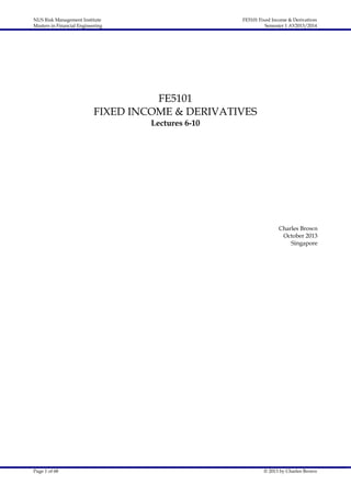
  • 21. NUS Risk Management Institute Masters in Financial Engineering FE5101 Fixed Income & Derivatives Semester 1 AY2013/2014 3.3.4 Volatility as a Parameter The BS formula is used to calculate an option price based on a set of inputs : – spot, interest rates (market data) – strike, tenor (contract terms) – volatility (model parameter) Volatility is not observable, while option prices are. 3.3.5 Implied Volatilities by Strike We can use the BS formula to invert an option price to give an implied volatility. By doing this to the entire set of option prices shown in the previous chart, a ‘volatility surface’ is obtained. Implied Volatilities by Strike and Tenor 21.00% Implied Volatility 19.00% 17.00% 15.00% 13.00% 11.00% 24M 9M 3M 1M 102.4975 O/N 98.3976 94.2977 90.1978 86.0979 81.9980 77.8981 73.7982 Strike 69.6983 61.4985 65.5984 9.00% Tenor It can be seen that this volatility surface is somewhat flatter than the price surface – it is more easily ‘parametrized’. The implied volatility surface can be further re-scaled by plotting the strike (K) axis in terms of LN(K/F) and the tenor (T) axis in terms of √T. The result is much flatter still, since these terms closely reflect what is in the BS formula – but still not completely flat. The volatility surface exhibits both a term structure and a ‘smile’. Page 21 of 68 © 2013 by Charles Brown
  • 22. NUS Risk Management Institute Masters in Financial Engineering FE5101 Fixed Income & Derivatives Semester 1 AY2013/2014 3.3.6 Characteristics of a Long Call Option The characteristics of a Call Option are reviewed, as an introduction to discussion of the drivers behind the term structure of implied volatility. Portfolio Value of an ATM Call Option 14000 12000 10000 8000 6000 4000 11.11% 9.18% 7.28% 5.41% 3.57% 1.77% 0.00% -1.74% -3.45% -5.13% -6.78% -8.41% -19.90% -10.00% -13.27% -16.58% -6.63% -9.95% 0.00% -3.32% 6.63% 3.32% 13.27% Vol Bump (absolute) 9.95% 0 16.58% 19.90% 2000 Spot Bump (relative) Portfolio Delta of an ATM Call Option 100000 90000 80000 70000 60000 50000 40000 30000 20000 Page 22 of 68 11.11% 9.18% 7.28% 5.41% 3.57% 1.77% 0.00% -1.74% -3.45% -5.13% -6.78% -8.41% -19.90% -10.00% -13.27% -16.58% -6.63% -9.95% 0.00% -3.32% 6.63% 13.27% 3.32% Vol Bump (absolute) 9.95% 0 16.58% 19.90% 10000 Spot Bump (relative) © 2013 by Charles Brown
  • 23. NUS Risk Management Institute Masters in Financial Engineering FE5101 Fixed Income & Derivatives Semester 1 AY2013/2014 Portfolio Gamma of an ATM Call Option 5000000 4500000 4000000 3500000 3000000 2500000 2000000 1500000 1000000 11.11% 9.18% 7.28% 5.41% 3.57% 1.77% 0.00% -1.74% -3.45% -5.13% -6.78% -8.41% -17.00% -10.00% -11.33% -14.17% -5.67% -8.50% 0.00% -2.83% 5.67% 11.33% 2.83% Vol Bump (absolute) 8.50% 0 14.17% 17.00% 500000 Spot Bump (relative) Portfolio Theta of an ATM Call Option 0 -5000 -10000 -15000 Note that both axes have been reversed for this graph for easy viewing -20000 -25000 Page 23 of 68 -10.00% -7.60% -5.13% -2.60% 0.00% 2.67% 5.41% 8.22% 16.58% 19.90% 11.11% 9.95% 13.27% 3.32% 6.63% 0.00% -6.63% -3.32% Vol Bump (absolute) -9.95% -19.90% -16.58% -13.27% -30000 Spot Bump (relative) © 2013 by Charles Brown
  • 24. NUS Risk Management Institute Masters in Financial Engineering FE5101 Fixed Income & Derivatives Semester 1 AY2013/2014 Portfolio Vega of an ATM Call Option 12000 10000 8000 6000 4000 19.90% 2000 14.93% 9.95% 4.98% 9.18% 7.28% 5.41% 3.57% 1.77% -1.74% -5.13% -6.78% -10.00% -19.90% -8.41% -14.93% -3.45% -9.95% 0.00% -4.98% 11.11% 0 0.00% Vol Bump (absolute) Spot Bump (relative) Portfolio Volga of an ATM Call Option 450000 400000 350000 300000 250000 200000 150000 100000 50000 19.90% 14.93% 0 9.95% 4.98% Page 24 of 68 -5.13% -6.78% -10.00% -19.90% -8.41% 9.18% 7.28% 5.41% 3.57% 1.77% -14.93% -1.74% -9.95% 0.00% -4.98% -3.45% Vol Bump (absolute) 11.11% -50000 0.00% Spot Bump (relative) © 2013 by Charles Brown
  • 25. NUS Risk Management Institute Masters in Financial Engineering FE5101 Fixed Income & Derivatives Semester 1 AY2013/2014 Portfolio Vanna of an ATM Call Option 1000000 800000 600000 400000 19.90% 16.58% 13.27% 9.95% 6.63% 3.32% Vol Bump 0.00% (absolute) -3.32% 200000 0 -200000 -400000 -6.63% -600000 -9.95% -13.27% -800000 -16.58% 9.18% 11.11% 5.41% 3.57% 1.77% 0.00% -1.74% -3.45% -5.13% -6.78% -8.41% -10.00% 7.28% -1000000 -19.90% Spot Bump (relative) Theta and Gamma Page 25 of 68 © 2013 by Charles Brown
  • 26. NUS Risk Management Institute Masters in Financial Engineering FE5101 Fixed Income & Derivatives Semester 1 AY2013/2014 3.4 Term Structure of Implied Volatility 3.4.1 Volatility Cones ATM Implied Volatility by Tenor 25.00% 23.00% ATM Implied Volatility 21.00% 19.00% 17.00% 15.00% 13.00% 11.00% 9.00% 7.00% 1 101 201 301 401 501 601 701 Tenor in Days 3.4.2 Term Structure - Drivers • Vols show mean reversion • Short Maturities: – do not have any vega exposures – driven by the relative benefits of gamma versus the costs of theta – a long option position is long gamma and profits from actual volatility through delta rebalancing; but is also short theta and loses from the passage of time (and vice versa) • Long Maturities: – – • do not have any gamma or theta exposures driven by supply and demand for vega (exposure to volatility moves) For both long and short maturities, implied volatility is traded using Delta Neutral Straddles Page 26 of 68 © 2013 by Charles Brown
  • 27. NUS Risk Management Institute Masters in Financial Engineering FE5101 Fixed Income & Derivatives Semester 1 AY2013/2014 3.4.3 Strategy Definition : Delta Neutral Straddle Buying a DELTA NEUTRAL STRADDLE involves: – buy 1x Call strike K – buy 1x Put strike K – K such that net delta (premium included) is zero  K  K1   K  K1       DNSTDL  C  Delta - Premium%  X %   P Delta - Premium%  X %          ATM ATM     The strike of a Delta Neutral Straddle can be formulated as: K  F e  1  2 T 2 + for counter ccy premium - for base ccy premium The  ATM term is referred to as the ‘at-the-money (atm) volatility’. It is used to describe the implied volatility used to price a Delta Neutral Straddle, whose strike is often referred to as the ‘atm strike’. We will see later that the market parametrizes the implied volatility smile by using just three volatilities:  ATM ,  RR ,  BF . Premium included delta The net delta for a straddle is calculated as the sum of the two option deltas less the sum of the two option premia (i.e. ‘premium included delta’), since the premium for a straddle is relatively large. The two premiums must be converted to %den by dividing the premium from the BS formula by spot, since the delta from the BS formula is in %den units. Terminology for units (DEN and NUM) Value and Greeks The following graphs show the value and greeks for a Delta Neutral Straddle, for a range of spot rates and implied volatilities: Page 27 of 68 © 2013 by Charles Brown
  • 28. NUS Risk Management Institute Masters in Financial Engineering FE5101 Fixed Income & Derivatives Semester 1 AY2013/2014 Portfolio Value of a DN Straddle 14000 12000 10000 8000 6000 4000 Page 28 of 68 11.11% 9.18% 7.28% 5.41% 3.57% 1.77% 0.00% -1.74% -3.45% -5.13% -6.78% -8.41% -10.00% -10.00% -6.67% -8.33% -3.33% -5.00% 0.00% Vol Bump (absolute) 0 -1.67% 10.00% 8.33% 6.67% 5.00% 3.33% 1.67% 2000 Spot Bump (relative) © 2013 by Charles Brown
  • 29. NUS Risk Management Institute Masters in Financial Engineering FE5101 Fixed Income & Derivatives Semester 1 AY2013/2014 Portfolio Delta of a DN Straddle 100000 80000 60000 40000 20000 0 -20000 -40000 -60000 11.11% 9.18% 7.28% 5.41% 3.57% 1.77% 0.00% -1.74% -3.45% -5.13% -6.78% -8.41% -10.00% -10.00% -6.67% -8.33% -3.33% -5.00% 0.00% Vol Bump (absolute) -100000 -1.67% 10.00% 8.33% 6.67% 5.00% 3.33% 1.67% -80000 Spot Bump (relative) Portfolio Gamma of a DN Straddle 3000000 2500000 2000000 1500000 1000000 Page 29 of 68 11.11% 9.18% 7.28% 5.41% 3.57% 1.77% 0.00% -1.74% -3.45% -5.13% -6.78% -8.41% -10.00% -10.00% -6.67% -8.33% -3.33% -5.00% 0.00% Vol Bump (absolute) 0 -1.67% 10.00% 8.33% 6.67% 5.00% 3.33% 1.67% 500000 Spot Bump (relative) © 2013 by Charles Brown
  • 30. NUS Risk Management Institute Masters in Financial Engineering FE5101 Fixed Income & Derivatives Semester 1 AY2013/2014 Portfolio Theta of a DN Straddle 0 -5000 -10000 -15000 -20000 -25000 -30000 -35000 11.11% 9.18% 7.28% 5.41% 3.57% 1.77% 0.00% -1.74% -3.45% -5.13% -6.78% -8.41% -10.00% -10.00% -6.67% -8.33% -3.33% -5.00% 0.00% Vol Bump (absolute) -45000 -1.67% 10.00% 8.33% 6.67% 5.00% 3.33% 1.67% -40000 Spot Bump (relative) Portfolio Vega of a DN Straddle 25000 20000 15000 10000 Page 30 of 68 11.11% 9.18% 7.28% 5.41% 3.57% 1.77% 0.00% -1.74% -3.45% -5.13% -6.78% -8.41% -10.00% -10.00% -6.67% -8.33% -3.33% -5.00% 0.00% Vol Bump (absolute) 0 -1.67% 10.00% 8.33% 6.67% 5.00% 3.33% 1.67% 5000 Spot Bump (relative) © 2013 by Charles Brown
  • 31. NUS Risk Management Institute Masters in Financial Engineering FE5101 Fixed Income & Derivatives Semester 1 AY2013/2014 Portfolio Volga of a DN Straddle 180000 160000 140000 120000 100000 80000 60000 40000 20000 11.11% 9.18% 7.28% 5.41% 3.57% 1.77% 0.00% -1.74% -3.45% -5.13% -6.78% -8.41% -10.00% -10.00% -6.67% -8.33% -3.33% -5.00% 0.00% Vol Bump (absolute) -20000 -1.67% 10.00% 8.33% 6.67% 5.00% 3.33% 1.67% 0 Spot Bump (relative) Portfolio Vanna of a DN Straddle 500000 400000 300000 200000 100000 0 -100000 -200000 -300000 11.11% 9.18% 7.28% 5.41% 3.57% 1.77% 0.00% -1.74% -3.45% -5.13% -6.78% -8.41% -10.00% -10.00% -6.67% -8.33% -3.33% -5.00% 0.00% Vol Bump (absolute) -500000 -1.67% 10.00% 8.33% 6.67% 5.00% 3.33% 1.67% -400000 Spot Bump (relative) 3.4.4 Strategy Definition : Calendar Spread • Buying a CALENDAR SPREAD involves: – – Page 31 of 68 buy 1x STDL maturity T1 sell 1x STDL maturity T2 © 2013 by Charles Brown
  • 32. NUS Risk Management Institute Masters in Financial Engineering FE5101 Fixed Income & Derivatives Semester 1 AY2013/2014 – where T2 > T1 – strikes often ATM for each tenor, or numerically equal 3.4.5 Forward volatility and no-arbitrage constraints The variance of a random variable X is its second central moment, the expected value of the squared deviation from the mean. In the GARCH spreadsheet, we calculated a variance for the daily returns (the daily variance) by taking an average of the squared returns for the sample: 1 n  S   2     ln i 1  n i  0  Si    2 The daily variance is an average, calculated by summing the realized squared daily returns and dividing by the number of returns. Variance measures how far a set of numbers (here, the returns) is spread out. Assume there are 252 daily returns in each year (and that these daily returns are independent and identically distributed). Then the variance for the annual returns (the annual variance) would be:  2  252   2 where  is the annualized volatility. (Volatility is always shown as annualized, unless explicitly stated otherwise.) The annual variance is calculated by multiplying the average daily variance by the number of days in one year. So the volatility implies an average daily variance, and vice versa. Equally for some period of T years, the variance would be:  2 T   252  T   2  T If we know the volatilities for tenors T1 and T2>T1 (where T0 is today):  T 0T 1 2  T1  T 0  2 T 0  T1  252  T1  T 0  T 0T 2 2  T 2  T 0  2 T 0  T 2  252  T 2  T 0  T 1T 2 2  T 2  T1  2 T1  T 2  252  T 2  T1 Page 32 of 68 © 2013 by Charles Brown
  • 33. NUS Risk Management Institute Masters in Financial Engineering FE5101 Fixed Income & Derivatives Semester 1 AY2013/2014 Since it is trivial to show the relationship between the average daily variances:  2 T 0  T 1  T 1  T 0   2 T 1  T 2  T 2  T 1   2 T 0  T 2  T 2  T 0 then  T 0T 1 2  T1  T 0   T 1T 2 2  T 2  T1   T 0T 2 2  T 2  T 0 and  T 1T 2 2  T 2  T1   T 0T 2 2  T 2  T 0   T 0T 1 2  T1  T 0 i.e. if we know the volatilities for two tenors T1 and T2, we can imply the volatility for the forward period between the two tenors. Furthermore, since variances cannot be negative, this introduces a constraint on the relationship between  T 0T 1  and  T 0T 2  :  T 0T 2 2  T 2  T 0   T 0T 1 2  T1  T 0 The constraint means that, while  T 0T 2  can be less than  T 0T 1  (i.e. the volatility term structure can have a negative slope), there is a limit to how much lower it can be. Noting that  2 T is a key term in the BS formula, this constraint is equivalent to saying that the cost of a calendar spread must be positive. It follows from this that the way to arbitrage a term structure whose slope is too negative is via the purchase of a calendar spread (buy the shorter tenor and sell the longer tenor) structured to result in a net receipt of premium. 3.4.6 Term Structure Interpolation See SS3. Page 33 of 68 © 2013 by Charles Brown
  • 34. NUS Risk Management Institute Masters in Financial Engineering FE5101 Fixed Income & Derivatives Semester 1 AY2013/2014 31% 29% 27% 25% 23% 21% 19% 17% 15% 0 90 180 270 360 BS Vol 450 540 630 720 Fwd Vol 3.4.7 Accounting for holidays and events See SS3. Page 34 of 68 © 2013 by Charles Brown
  • 35. NUS Risk Management Institute Masters in Financial Engineering FE5101 Fixed Income & Derivatives Semester 1 AY2013/2014 27.00% 26.50% 26.00% 25.50% 25.00% 24.50% 24.00% 23.50% 30 37 44 51 58 vol 3.5 Further Reading Reference “Why we have never used the BSM option pricing formula”, Espen Gaarder Haug and Nassim Taleb “040522 A note on sufficient conditions for no arbitrage”, Peter Carr and Dilip B. Madan “041102 Implied Vol Constraints”, Peter Carr “060801 Volatility Surfaces Theory, Rules of Thumb, and Empirical Evidence”, Toby Daglish, John Hull and Wulin Suo Page 35 of 68 © 2013 by Charles Brown
  • 36. NUS Risk Management Institute Masters in Financial Engineering 4 FE5101 Fixed Income & Derivatives Semester 1 AY2013/2014 The Implied Volatility Surface : Smile 4.1 Objectives for this Section 4.2 The Observed Smile The following graph shows a range of option prices computed using the Black-Scholes formula and a single volatility for all strikes and tenors. For strikes above the current market, the options are Calls, and for strikes below the current market, the options are Puts. Option Prices for Flat Vol (BS) 6.000 5.000 Price 4.000 3.000 2.000 1.000 24M 9M 3M 1M 102.4953 O/N 94.2957 98.3955 86.0961 90.1959 77.8965 81.9963 69.6968 Strike 73.7966 61.4972 65.5970 0.000 Tenor The next graph shows, by comparison, option prices for the same underlying as they are observed in the market. Option Prices in $ by Strike and Tenor 8.000 7.000 6.000 Price 5.000 4.000 3.000 2.000 1.000 Page 36 of 68 102.4975 O/N 1W 1M 2M 3M 6M 9M 12M 24M 98.3976 94.2977 86.0979 90.1978 77.8981 69.6983 81.9980 Strike 73.7982 61.4985 65.5984 0.000 Tenor © 2013 by Charles Brown
  • 37. NUS Risk Management Institute Masters in Financial Engineering FE5101 Fixed Income & Derivatives Semester 1 AY2013/2014 By visual comparison of the two price surfaces, the overall shape is at first sight very similar. While the two surfaces are clearly not the same, it is difficult to pinpoint any characteristic difference between the two. Nevertheless, the market is clearly not using the same volatility parameter for all strikes and tenors. How is this question to be approached? We can try to describe this set of observed option prices in terms of as few model parameters as possible (i.e. a ‘parsimonious’ or minimalistic model of the market, similar to Nelson-Siegel for the yield curve). Therefore we switch from the price space to the implied volatility space to try and remove any ‘noise’ and focus on the residual marginal underlying differences between these computed and observed prices, bearing in mind that in this implied volatility space the set of computed option prices in the first graph would be entirely flat. The following graph shows the set of observed option prices in the second graph, in terms of their implied volatilities. The option price for each strike and tenor has been fed into the Black-Scholes formula, and a volatility parameter has been implied from this desired output (hence ‘implied volatility’). In this graph, it is now very obvious where this volatility surface deviates from an entirely flat surface; and also some structure is visible: versus tenors (term structure) and versus strikes (smile). Implied Volatilities by Strike and Tenor 21.00% Implied Volatility 19.00% 17.00% 15.00% 13.00% 11.00% Page 37 of 68 24M 9M 3M 1M 102.4975 O/N 98.3976 90.1978 94.2977 86.0979 77.8981 69.6983 81.9980 Strike 73.7982 61.4985 65.5984 9.00% Tenor © 2013 by Charles Brown
  • 38. NUS Risk Management Institute Masters in Financial Engineering FE5101 Fixed Income & Derivatives Semester 1 AY2013/2014 The Black-Scholes formula is not scaled in terms of the strike (K) or tenor (T) but rather in terms of LnK  and T , so re-scaling the x and y axes should remove any artefacts in the surface due to this scaling. The graph below shows the same volatilities versus LnK  and T . The result is much smoother, which is a good result as this means the surface will be easier to parametrize. Implied Volatilities by Delta and Tenor Implied Volatility 20.00% 18.00% 16.00% 14.00% 12.00% 10.00% 24M 9M 3M 1M 3.50% O/N 10.00% 30.00% 20.00% 50.00% 40.00% 40.00% 20.00% Delta 30.00% 3.50% 10.00% 8.00% Tenor 4.3 The Smile – Constraints The following section describes the three ways that option prices are constrained along the strike axis. 4.3.1 Put Spreads and Call Spreads Observation : Put Spreads must have a +ve value, otherwise there is an arbitrage. Observation : Call Spreads must have a +ve value, otherwise there is an arbitrage. +P(K+dK) – P(K) ≥ 0  -F(K+dK) + C(K+dK) - P(K) ≥ 0  -F(K) + dK + C(K+dK) - P(K) ≥ 0  -C(K) + dK + C(K+dK) ≥ 0  +C(K) - C(K+dK) ≤ dK +C(K) – C(K+dK) ≥ 0  +C(K) - F(K+dK) - P(K+dK) ≥ 0  +C(K) - F(K) + dK - P(K+dK) ≥ 0  +P(K) + dK - P(K+dK) ≥ 0  +P(K+dK) - P(K) ≤ dK This also tells us, via Put-Call Parity, that a Call Spread must be worth at most the difference between its strikes. This also tells us that, via Put-Call Parity, a Put Spread must be worth at most the difference between its strikes. These constraints are on the future value of the spreads. They also imply constraints on individual option values : Page 38 of 68 © 2013 by Charles Brown
  • 39. NUS Risk Management Institute Masters in Financial Engineering FE5101 Fixed Income & Derivatives Semester 1 AY2013/2014 P(K+dK) ≥ P(K) As strike is increased, the premium for a Put option must increase. C(K) ≥ C(K+dK) As strike is decreased, the premium for a Call option must increase. And by Put-Call Parity : And by Put-Call Parity : C(K+dK) ≥ C(K) - dK As strike is increased, the premium for a Call option cannot fall faster than the strike is rising. P(K) ≥ P(K+dK) - dK As strike is decreased, the premium for a Put option cannot fall faster than the strike is falling. 4.3.2 Butterflies The second constraint is based on the observation that a Butterfly must have a positive future value. A Butterfly strategy is a spread of two Call spreads (or two Put spreads). In this case, the two Call spreads will have equal notionals and the Butterfly will be ‘symmetric’ (i.e. the three strikes will be equally spaced), but the constraint applies equally to ‘asymmetric’ Butterflies where the constituent Call spreads have different notionals and the three strikes are not equally spaced. The constraint on the minimum value of the Butterfly can be written as follows: Observation : Butterfly (of Put spreads) must have a +ve value, otherwise there is an arbitrage. Observation : Butterfly (of Call spreads) must have a +ve value, otherwise there is an arbitrage. {+P(K+dK)–P(K)} – {+P(K)-P(K-dK)} ≥0  + P(K+dK) – 2*P(K) + P(K-dK) ≥0  + P(K+dK) – P(K) ≥+ P(K) - P(K-dK) {+C(K-dK)–C(K)} – {+C(K)-C(K+dK)} ≥0  + C(K-dK) – 2*C(K) + C(K+dK) ≥0  + C(K-dK) – C(K) ≥+ C(K) - C(K+dK)   As strike is increased, the rate of increase of the premium for a Put option must increase. As strike is decreased, the rate of decrease of the premium for a Put option must decrease.   As strike is increased, the rate of decrease of the premium for a Call option must decrease. As strike is decreased, the rate of increase of the premium for a Call option must increase. What this means is that the relationship between the option price and the strike is convex. Page 39 of 68 © 2013 by Charles Brown
  • 40. NUS Risk Management Institute Masters in Financial Engineering FE5101 Fixed Income & Derivatives Semester 1 AY2013/2014 4.3.3 Option Price Asymptotes While the Butterfly price constraint suggests that, for example, a Put option’s premium is increasing endlessly for higher strikes, this does not mean that the premium tends to infinity for very high strikes; instead it tends towards an asymptote. For strikes tending to zero: Observation : a Call with a notional of 1 den and strike K of zero on an underlying with units num den must have a future value equal to 1 den. This Call option gives the owner the right to receive at maturity 1 den at no cost. Thus its ˆ future value C K  must be equal to 1 den, with the assumption that the probability of ST<0 is zero. Since F is the current forward price and the notional is 1 den, this future value is equivalent to a future value of 1 den  F num den or simply F. In num den 1 den  F num den units, using Put-Call Parity: ˆ  C 0  F ˆ ˆ   F 0  P0  F ˆ ˆ   P0  F  F 0  0   As strike tends to zero, the future value of a Call option tends to the forward price F. As strike tends to zero, the future value of a Put option tends to zero. For strikes tending to infinity: Observation : a Call with a notional of 1 num and a strike K * of zero on an underlying with units den num must have a future value equal to 1 num. This Call option gives the owner the right to receive at maturity 1 num at no cost. Thus its future value must be equal to 1 num, with the assumption that the probability of S*T<0 is zero. Since F *  1 F is the current forward price and the notional is 1 num, this future value is equivalent to den 1 num  F * num but we need to express this in terms of den F * num  Page 40 of 68 num num den den  F * num den : F * den  F 1 num den 1 num  K * num 1 num K * den © 2013 by Charles Brown
  • 41. NUS Risk Management Institute Masters in Financial Engineering K * is zero, in and since num FE5101 Fixed Income & Derivatives Semester 1 AY2013/2014 den units the value will be ∞. This Call C*(K*) on underlying with units with units num den : and equally In   num den den num is equivalent to a Put P(K) on underlying + C*(K*=0) = +P(K=∞) + P*(K*=0) = +C(K=∞) units: ˆ  C * 0   1 ˆ   P  K* ˆ ˆ   F * 0   P* 0   1 * K ˆ ˆ ˆ   P* 0   1 *  F * 0   0  C   K As strike tends to ∞, the future value of a Call option tends to zero. As strike tends to ∞, the future value of a Put option tends to K. 4.3.4 Examples (from Hull) Page 41 of 68 © 2013 by Charles Brown
  • 42. NUS Risk Management Institute Masters in Financial Engineering FE5101 Fixed Income & Derivatives Semester 1 AY2013/2014 4.4 The Smile - Drivers 4.4.1 Principal Component Analysis Page 42 of 68 © 2013 by Charles Brown
  • 43. NUS Risk Management Institute Masters in Financial Engineering FE5101 Fixed Income & Derivatives Semester 1 AY2013/2014 4.4.2 Quoting Conventions The Smile can be quoted “sticky delta” or “sticky strike” basis according to liquidity and precedent (if rigidly interpreted, both would be open to arbitrage - real world is somewhere inbetween). 4.4.3 Smile Dynamics and Exotics Forward dynamics of the smile matter a lot for exotic options.  K , T  • The Vol Surface gives us: • But we would like to have: • For example, to calculate the option delta:  S, t  V S , T , K ,  S , K  S V S , T , K ,  S , K   S , K    h1     S , K  S  Deterministic Smiles • Deterministic Smile  det   det t , T , K , S t  • Sticky Smile (Sticky Strike) • Floating Smile (Sticky Delta) • Forward-Propagated Smile  fwd   fwd  T  t ,   stick   stick t , T , K    float   float  t , T ,     K St K St         4.4.4 Interpretations of the Smile As Probability Distribution As Risk Premia The Smile represents the marginal risk premium charged for risks not incorporated in Black-Scholes (principally, that volatility is not constant and there is consequently a hedging cost associated with it). Page 43 of 68 © 2013 by Charles Brown
  • 44. NUS Risk Management Institute Masters in Financial Engineering FE5101 Fixed Income & Derivatives Semester 1 AY2013/2014 4.5 The Smile - Skew  The Skew (asymmetry) causes vols for higher strikes to be higher (or lower) than those for lower strikes  It is (mostly) an implicit correction for the correlation between implied volatility and the underlying asset price  It is traded using Risk Reversals, a pure Vanna position 4.5.1 Strategy Definition : Risk Reversal K  K2   K  K3       RR25%   C  Delta  25%   P Delta  25%          1 1 ATM   BF  2  RR  ATM   BF  2  RR    This is not sufficient information to find consistent vols for 25 delta Put and 25 delta Call as individual options (whose strikes will not be K2, K3). The risks of a Risk Reversal are shown below. Portfolio Value of a 25d Risk Reversal 8000 6000 4000 2000 0 -2000 -4000 Page 44 of 68 11.11% 9.18% 7.28% 5.41% 3.57% 1.77% 0.00% -1.74% -3.45% -5.13% -6.78% -8.41% -10.00% -10.00% -6.67% -8.33% -3.33% -5.00% 0.00% Vol Bump (absolute) -8000 -1.67% 10.00% 8.33% 6.67% 5.00% 3.33% 1.67% -6000 Spot Bump (relative) © 2013 by Charles Brown
  • 45. NUS Risk Management Institute Masters in Financial Engineering FE5101 Fixed Income & Derivatives Semester 1 AY2013/2014 Portfolio Delta of a 25d Risk Reversal 100000 90000 80000 70000 60000 50000 40000 30000 20000 11.11% 9.18% 7.28% 5.41% 3.57% 1.77% 0.00% -1.74% -3.45% -5.13% -6.78% -8.41% -10.00% -10.00% -6.67% -8.33% -3.33% -5.00% 0.00% Vol Bump (absolute) 0 -1.67% 10.00% 8.33% 6.67% 5.00% 3.33% 1.67% 10000 Spot Bump (relative) Portfolio Gamma of a 25d Risk Reversal 1500000 1000000 500000 0 -500000 -1000000 Page 45 of 68 11.11% 9.18% 7.28% 5.41% 3.57% 1.77% 0.00% -1.74% -3.45% -5.13% -6.78% -8.41% -10.00% -10.00% -6.67% -8.33% -3.33% -5.00% 0.00% Vol Bump (absolute) -2000000 -1.67% 10.00% 8.33% 6.67% 5.00% 3.33% 1.67% -1500000 Spot Bump (relative) © 2013 by Charles Brown
  • 46. NUS Risk Management Institute Masters in Financial Engineering FE5101 Fixed Income & Derivatives Semester 1 AY2013/2014 Portfolio Theta of a 25d Risk Reversal 10000 5000 0 -5000 11.11% 9.18% 7.28% 5.41% 3.57% 1.77% 0.00% -1.74% -3.45% -5.13% -6.78% -8.41% -10.00% -10.00% -6.67% -8.33% -3.33% -5.00% 0.00% Vol Bump (absolute) -15000 -1.67% 10.00% 8.33% 6.67% 5.00% 3.33% 1.67% -10000 Spot Bump (relative) Portfolio Vega of a 25d Risk Reversal 15000 10000 5000 0 -5000 Page 46 of 68 11.11% 9.18% 7.28% 5.41% 3.57% 1.77% 0.00% -1.74% -3.45% -5.13% -6.78% -8.41% -10.00% -10.00% -6.67% -8.33% -3.33% -5.00% 0.00% Vol Bump (absolute) -15000 -1.67% 10.00% 8.33% 6.67% 5.00% 3.33% 1.67% -10000 Spot Bump (relative) © 2013 by Charles Brown
  • 47. NUS Risk Management Institute Masters in Financial Engineering FE5101 Fixed Income & Derivatives Semester 1 AY2013/2014 Portfolio Volga of a 25d Risk Reversal 80000 60000 40000 20000 0 -20000 -40000 -60000 11.11% 9.18% 7.28% 5.41% 3.57% 1.77% 0.00% -1.74% -3.45% -5.13% -6.78% -8.41% -10.00% -10.00% -6.67% -8.33% -3.33% -5.00% 0.00% Vol Bump (absolute) -100000 -1.67% 10.00% 8.33% 6.67% 5.00% 3.33% 1.67% -80000 Spot Bump (relative) Portfolio Vanna of a 25d Risk Reversal 500000 400000 300000 200000 100000 0 -100000 11.11% 9.18% 7.28% 5.41% 3.57% 1.77% 0.00% -1.74% -3.45% -5.13% -6.78% -8.41% -10.00% -10.00% -6.67% -8.33% -3.33% -5.00% 0.00% Vol Bump (absolute) -300000 -1.67% 10.00% 8.33% 6.67% 5.00% 3.33% 1.67% -200000 Spot Bump (relative) 4.5.2 Vanna The formula for Vanna (under BS) is:  2V d  e  D (T ) N ' (d1 )  2 S  Page 47 of 68 © 2013 by Charles Brown
  • 48. NUS Risk Management Institute Masters in Financial Engineering FE5101 Fixed Income & Derivatives Semester 1 AY2013/2014 Vanna is the second derivative of the Price with respect to Volatility and Spot. It is dDelta/dVol or dVega/dSpot. Hedge vanna with Risk Reversals. 4.6 The Smile - Wings  The Wings (kurtosis, fat tails) causes vols for otm strikes to be higher than those for an atm strike  It is an implicit correction for the higher-than-'lognormal' possibility of jumps  It is traded using Vega Neutral Butterflies, a pure Volga position 4.6.1 Strategy Definition : Market or 1Vol Strangle K  K4   K  K5       STGL25%   C  Delta  25%   P Delta  25%          ATM   BF  ATM   BF    This is not sufficient information to find consistent vols for 25 delta Put and 25 delta Call as individual options (whose strikes will not be K4, K5). 4.6.2 Volga The formula for Volga (under BS) is:  2V dd  S T  e  D (T ) N ' (d1 )  1 2 2   Volga is the second derivative of the Price with respect to Volatility. It is d2Price/dVol2 or dVega/dVol, also known as volgamma. Hedge volga with VN Butterflies. 4.6.3 Strategy Definition : Vega Neutral Butterfly  VNBF   w  STGL    ATM   BF   1  DNSTDL    ATM  with w such that net vega is zero. The risks of a Vega Neutral Butterfly are shown below: Page 48 of 68 © 2013 by Charles Brown
  • 49. NUS Risk Management Institute Masters in Financial Engineering FE5101 Fixed Income & Derivatives Semester 1 AY2013/2014 Portfolio Value of a VNBF 0 -500 -1000 -1500 -2000 -2500 -3000 -3500 11.11% 9.18% 7.28% 5.41% 3.57% 1.77% 0.00% -1.74% -3.45% -5.13% -6.78% -8.41% -10.00% -10.00% -6.67% -8.33% -3.33% -5.00% 0.00% Vol Bump (absolute) -4500 -1.67% 10.00% 8.33% 6.67% 5.00% 3.33% 1.67% -4000 Spot Bump (relative) Portfolio Delta of a VNBF 20000 15000 10000 5000 0 -5000 -10000 -15000 Page 49 of 68 11.11% 9.18% 7.28% 5.41% 3.57% 1.77% 0.00% -1.74% -3.45% -5.13% -6.78% -8.41% -10.00% -10.00% -6.67% -8.33% -3.33% -5.00% 0.00% Vol Bump (absolute) -25000 -1.67% 10.00% 8.33% 6.67% 5.00% 3.33% 1.67% -20000 Spot Bump (relative) © 2013 by Charles Brown
  • 50. NUS Risk Management Institute Masters in Financial Engineering FE5101 Fixed Income & Derivatives Semester 1 AY2013/2014 Portfolio Gamma of a VNBF 1000000 800000 600000 400000 200000 0 -200000 -400000 -600000 -800000 11.11% 9.18% 7.28% 5.41% 3.57% 1.77% 0.00% -1.74% -3.45% -5.13% -6.78% -8.41% -10.00% -10.00% -6.67% -8.33% -3.33% -5.00% 0.00% Vol Bump (absolute) -1200000 -1.67% 10.00% 8.33% 6.67% 5.00% 3.33% 1.67% -1000000 Spot Bump (relative) Portfolio Theta of a VNBF 4000 2000 0 -2000 -4000 -6000 Page 50 of 68 11.11% 9.18% 7.28% 5.41% 3.57% 1.77% 0.00% -1.74% -3.45% -5.13% -6.78% -8.41% -10.00% -10.00% -6.67% -8.33% -3.33% -5.00% 0.00% Vol Bump (absolute) -10000 -1.67% 10.00% 8.33% 6.67% 5.00% 3.33% 1.67% -8000 Spot Bump (relative) © 2013 by Charles Brown
  • 51. NUS Risk Management Institute Masters in Financial Engineering FE5101 Fixed Income & Derivatives Semester 1 AY2013/2014 Portfolio Vega of a VNBF 10000 8000 6000 4000 2000 0 -2000 -4000 11.11% 9.18% 7.28% 5.41% 3.57% 1.77% 0.00% -1.74% -3.45% -5.13% -6.78% -8.41% -10.00% -10.00% -6.67% -8.33% -3.33% -5.00% 0.00% Vol Bump (absolute) -8000 -1.67% 10.00% 8.33% 6.67% 5.00% 3.33% 1.67% -6000 Spot Bump (relative) Portfolio Volga of a VNBF 150000 100000 50000 0 -50000 Page 51 of 68 11.11% 9.18% 7.28% 5.41% 3.57% 1.77% 0.00% -1.74% -3.45% -5.13% -6.78% -8.41% -10.00% -10.00% -6.67% -8.33% -3.33% -5.00% 0.00% Vol Bump (absolute) -150000 -1.67% 10.00% 8.33% 6.67% 5.00% 3.33% 1.67% -100000 Spot Bump (relative) © 2013 by Charles Brown
  • 52. NUS Risk Management Institute Masters in Financial Engineering FE5101 Fixed Income & Derivatives Semester 1 AY2013/2014 Portfolio Vanna of a VNBF 500000 400000 300000 200000 100000 0 -100000 -200000 -300000 11.11% 9.18% 7.28% 5.41% 3.57% 1.77% 0.00% -1.74% -3.45% -5.13% -6.78% -8.41% -10.00% -10.00% -6.67% -8.33% -3.33% -5.00% 0.00% Vol Bump (absolute) -500000 -1.67% 10.00% 8.33% 6.67% 5.00% 3.33% 1.67% -400000 Spot Bump (relative) 4.6.4 Butterfly variants Symmetric Asymmetric Weighted by Vega 7.5 2.5 2.5 -2.5 VALUE 12.5 7.5 VALUE 12.5 7.5 VALUE 12.5 -2.5 2.5 -2.5 -7.5 -7.5 -7.5 -12.5 -12.5 -12.5 75 80 85 90 95 100 105 110 115 120 125 UNDERLYING 75 80 85 90 95 100 105 110 115 120 125 75 80 85 90 UNDERLYING 95 100 105 110 115 120 125 UNDERLYING 12.5 VALUE 7.5 2.5 -2.5 -7.5 -12.5 75 80 85 90 95 100 105 110 115 120 125 UNDERLYING 4.7 Further Reading Reference “020204 Dynamics of Implied Volatility Surfaces”, Rama Cont and Jose da Fonseca “100320 FX Volatility Smile Construction”, Dimitri Reiswich and Uwe Wystup Page 52 of 68 © 2013 by Charles Brown
  • 53. NUS Risk Management Institute Masters in Financial Engineering FE5101 Fixed Income & Derivatives Semester 1 AY2013/2014 “2005 Consistent Pricing of FX Options”, Antonio Castagna and Fabio Mercurio “Implied Volatility - Statics, Dynamics, and Probabilistic Interpretation”, Roger Lee Page 53 of 68 © 2013 by Charles Brown
  • 54. NUS Risk Management Institute Masters in Financial Engineering 5 FE5101 Fixed Income & Derivatives Semester 1 AY2013/2014 Smile Interpolation, Extrapolation and Fitting 5.1 Objectives for this Section 5.2 The Market Smile The market prices for the three market structures (  ATM ,  RR ,  BF ) are exogenous in the sense that they are driven by supply and demand (for vega, vanna and volga as we will see later). These three volatility quotes constitute the market smile. However, each of these three market prices is for a pair of options, but we want to be able to derive a volatility consistent with these market prices for an individual option with any strike, i.e. an interpolated function  K  . Two separate methods of doing this are presented: (i) The Equivalent Smile : find three points on  K  that are consistent with the market smile and interpolate through those points using the traditional methods (polynomial etc.) (ii) The Vanna-Volga Model : extract the implied vega risk premia from the market smile and use these risk premia to generate  K  5.3 The Equivalent Smile We need a smile function  K  with three defined points  x1 ,  x2 ,  x3 , calibrated such that the smile function gives the same $ prices as the market smile for the three market structures - the Delta-Neutral Straddle, the 25-delta Risk Reversal, and the 25-Delta Strangle. In practice, the three defined points are taken to be for the strike of a 25-delta Put, the strike of an ATM option, and the strike of a 25-delta Call. These three defined points on  K  cannot be implied directly from the market smile because the three market structures actually generate five different strikes : the market Page 54 of 68 © 2013 by Charles Brown
  • 55. NUS Risk Management Institute Masters in Financial Engineering FE5101 Fixed Income & Derivatives Semester 1 AY2013/2014 risk reversal has two strikes K2 and K3, the market strangle has a further two strikes K4 and K5, and thus a lone option cannot be replicated by any combination of the two structures. The market gives the following prices (sticky delta): We need three points (strike,vol) to be able to interpolate: so that we can find the vol for any strike: Vol by Strike 40% 30% 20% 10% 0% 80 85 90 95 100105 110 115 120  ATM  RR  BF  25dP  ATM  25dC This calibration can be represented formulaically as follows, where the LHS is the $ price of the market structure using the market smile and the RHS is the $ price of the market structure using the smile function  K  : Market STDLDN   Put K DN  K1, ATM    Call K DN  K1, ATM     Put K1, ( K1)    Call K1, ( K1)  Market RR25d     Put  K 25 D  K 2, ATM  RR 2        Call  K 25 D  K 3, ATM  RR 2       Put K 2, ( K 2)    Call K 3, ( K 3)   Market STGL25d   Put K 25 D  K 4, ATM   BF    Call K 25 D  K 5, ATM   BF     Put K 4, ( K 4)    Call K 5, ( K 5)  where Π() is the price of an option using the BS formula Assuming some polynomial or other function to generate the smile function the unknowns are the three defined points  K  ,  25 DP ,  ATM ,  25 DC on  K  . We need to solve for these three, such that the above equalities are met, and our  K  is then arbitrage-free (at least with respect to the market smile – we have assumed that the market smile itself is arbitrage-free in the first place!). Page 55 of 68 © 2013 by Charles Brown
  • 56. NUS Risk Management Institute Masters in Financial Engineering FE5101 Fixed Income & Derivatives Semester 1 AY2013/2014 5.3.1 Definitions It would be quite possible to solve directly for (or calibrate) the three defined points  25 DP ,  ATM ,  25 DC . We would make an initial guess for these, imply the three respective strikes, use a polynomial (or other interpolation method) to extract the volatilities for the five strikes of the market structures, and test whether the $ prices match or not. In practice however, a so-called ‘Equivalent Smile’ is used for the calibration process, since the structures we are pricing are the market structures, and the calibration parameters should ideally reflect that (i.e. we want as strong a link as possible between the inputs and the outputs). The Equivalent Smile is defined as:  EQRR   25 DC   25 DP  EQBF   25 DC   25 DP 2   ATM and thus  25 DP   ATM   EQBF  1  EQRR 2  25 DC   ATM   EQBF  1  EQRR 2 In this case, the ‘Equivalent Risk Reversal’ and ‘Equivalent Strangle’ actually do share the same pair of strikes and we can combine them to get a construction consisting of a single strike only, and thus imply a volatility unique to that strike. 5.3.2 Exercise : Reconstruct the Smile Assume the following Equivalent Smile:  ATM  32.00%  EQRR  4.00%  EQBF  2.00% Calculate Vols for: the ATM strike? the 25D Put strike? Page 56 of 68 © 2013 by Charles Brown
  • 57. NUS Risk Management Institute Masters in Financial Engineering FE5101 Fixed Income & Derivatives Semester 1 AY2013/2014 the 25D Call strike? 5.3.3 Exercise : Deconstruct the Smile Assume the following Smile: Option 25D Put ATM 25D Call Strike 75.25 80.00 85.50 Vol 35% 32% 31% Price $1.30 $2.75 $1.00 Calculate Vols and Prices for: the DN Straddle? the Equivalent Strangle? the Equivalent Risk Reversal? 5.4 Solving for the Equivalent Smile Graphically: Page 57 of 68 © 2013 by Charles Brown
  • 58. NUS Risk Management Institute Masters in Financial Engineering Calibration of smile to market showing market vols for market instruments 70% 60% equivalent smile calibrated to market rr, stgl 50% Volatility FE5101 Fixed Income & Derivatives Semester 1 AY2013/2014 market rr market stgl 40% 30% 20% dn straddle 10% 0% 0.9000 1.1000 1.3000 25dP and 25dC 1.5000 1.7000 1.9000 Strike 70% Calibration of smile to market showing equivalent smile vols for market instruments 60% equivalent smile calibrated to market rr, stgl 50% market rr Volatility market stgl 40% 30% 20% 25dP and 25dC dn straddle 10% 0% 0.9000 1.1000 1.3000 1.5000 1.7000 1.9000 Strike Page 58 of 68 © 2013 by Charles Brown
  • 59. NUS Risk Management Institute Masters in Financial Engineering FE5101 Fixed Income & Derivatives Semester 1 AY2013/2014 Calibrated Risk Reversal prices Market Risk Reversal & Equivalent Risk Reversal (market prices vs equivalent smile prices) 0.1800 equivalent smile (puts) equivalent smile (calls) 0.1600 Price 0.1400 0.1200 0.1000 market risk reversal 0.0800 0.0600 0.0400 0.90 equivalent risk reversal 1.10 1.30 1.50 1.70 1.90 Strike Calibrated Strangle prices Market Strangle & Equivalent Strangle (market prices vs equivalent smile prices) 0.1800 equivalent smile (puts) equivalent smile (calls) 0.1600 Price 0.1400 0.1200 0.1000 market strangle 0.0800 0.0600 0.0400 0.90 equivalent strangle 1.10 1.30 1.50 1.70 1.90 Strike Page 59 of 68 © 2013 by Charles Brown
  • 60. NUS Risk Management Institute Masters in Financial Engineering FE5101 Fixed Income & Derivatives Semester 1 AY2013/2014 5.5 The VannaVolga Model 5.5.1 Pricing with the Equivalent Smile CALCULATE OPTION SMILE PRICE BY VANNAVOLGA EQUIVALENT SMILE 25dP 27.55% 89.2870 13.9625 25.00% vol strike call price BS vol BS price BS premdelta BS gamma BS theta BS vega BS volga BS vanna ATM 25.00% 98.4211 7.8715 25.00% 13.3933 77% 0.017 -5.374 21.910 34.634 -0.670 7.8715 57% 0.022 -6.875 28.029 -0.001 0.000 OPTION 25dC 24.49% 114.2446 2.3953 25.00% (Call) 24.311% 112.00 2.8335 25.00% 2.5127 26% 0.018 -5.630 22.951 50.388 1.074 3.0016 29% 0.019 -6.019 24.538 38.798 0.996 ^ this is in fact a 75DC not a 25DP VANNA-VOLGA PRICER FOR SINGLE EUROPEAN OPTION BY 3 OPTIONS 25.00% 21.910 34.634 -0.670 25.00% 28.029 -0.001 0.000 25.00% 22.951 50.388 1.074 25dC UNKNOWN 25.00% 24.538 38.798 0.996 WEIGHT 0.1196 W BSV VEGA 2.621 W BSV VOLGA 4.144 W BSV VANNA -0.080 -0.2711 -7.600 0.000 0.000 -0.8522 -19.559 -42.942 -0.916 1.0000 24.538 38.798 0.996 0.000 0.000 0.000 BSV PRICE SMILE PRICE SMILE ADJ W SMILE ADJ 7.8715 7.8715 0.0000 0.0000 2.5127 2.3953 -0.1173 0.1000 3.0016 2.8335 -0.1681 -0.1681 0.0000 BS VOL (BSV) BSV VEGA BSV VOLGA BSV VANNA 25dP 13.3933 13.9625 0.5692 0.0681 ATM TOTALS 5.5.2 Pricing with market structures CALCULATE OPTION SMILE PRICE BY VANNAVOLGA MARKET SMILE put vol put strike put price BS vol BS price BS premdelta BS gamma BS theta BS vega BS volga BS vanna call vol call strike call price BS vol BS price BS premdelta BS gamma BS theta BS vega BS volga BS vanna DNSTDL 25.00% 98.4211 6.2926 25.00% 6.2926 -43% 0.022 -6.875 28.029 -0.001 0.000 25.00% 98.4211 7.8715 25.00% 7.8715 57% 0.022 -6.875 28.029 -0.001 0.000 25DRR 26.50% 89.6101 3.1130 25.00% 2.7760 -24% 0.017 -5.453 22.229 32.890 -0.655 23.50% 113.5666 2.3065 25.00% 2.6526 27% 0.018 -5.751 23.446 46.911 1.054 OPTION (Call) 2.8230 -24% 0.018 -5.490 22.381 32.051 -0.647 24.311% 112.00 2.8335 2.3064 24% 0.017 -5.434 22.154 55.721 1.101 25.00% 56.058 -0.002 0.000 25.00% 1.217 14.022 1.708 25.00% 0.000 -110.486 -0.572 25.00% 24.538 38.798 0.996 (Call) TOTALS WEIGHT -0.4272 W BSV VEGA -23.947 W BSV VOLGA 0.001 W BSV VANNA 0.000 25DSTGL 26.00% 89.7660 3.0484 25.00% 26.00% 115.3049 2.5306 25.00% VANNA-VOLGA PRICER FOR SINGLE EUROPEAN OPTION BY MARKET STRUCTURES -0.4859 -0.591 -6.813 -0.830 0.2895 0.000 -31.986 -0.166 1.0000 24.538 38.798 0.996 -0.001 0.000 0.000 BSV PRICE MKT PRICE MKT ADJ W MKT ADJ -0.1234 -0.8064 -0.6831 0.3319 7.707 7.142 -0.5659 -0.1638 3.0016 2.8335 -0.1681 -0.1681 0.0000 BS VOL (BSV) BSV VEGA BSV VOLGA BSV VANNA DNSTDL 14.1641 14.1641 0.0000 0.0000 25DRR VNBF 25.00% 3.0016 29% 0.019 -6.019 24.538 38.798 0.996 VEGA NEUTRAL BUTTERFLY BSV VEGA WEIGHT W BSV VEGA DNSTDL 56.058 1.0000 56.058 25DSTGL 44.534 -1.2588 -56.058 0.000 5.5.3 Pricing directly by risk MARKET PRICE OF RISK WEIGHT W BSV VEGA W BSV VOLGA W BSV VANNA W BSV PRICE W MKT PRICE W MKT ADJ ADJUST PER UNIT OF RISK Option putcall strike BS price Smile Price Smile Vol Page 60 of 68 c 112.00 3.002 TOTALS DNSTDL 25DRR VNBF PORTFOLIO 1 : NEUTRAL IN VEGA AND VOLGA -0.0217 1.0000 0.1269 -1.2171 1.2171 0.0000 0.0000 0.0000 14.0217 -14.0215 0.0003 0.0000 1.7083 -0.0726 1.6357 -0.3075 -0.1234 0.9781 -0.3075 -0.8064 0.9063 0.0000 -0.6831 -0.0718 -0.755 -0.4615 (VANNA) TOTALS DNSTDL 25DRR VNBF PORTFOLIO 2 : NEUTRAL IN VEGA AND VANNA -0.0073 0.3349 1.0000 -0.4076 0.4076 0.0000 0.0000 0.0000 4.6963 -110.4860 -105.7897 0.0000 0.5722 -0.5720 0.0001 -0.1030 -0.0413 7.7074 -0.1030 -0.2701 7.1415 0.0000 -0.2288 -0.5659 -0.795 0.0075 (VOLGA) BS volga Volga Adj BS vanna Vanna Adj 38.798 0.2915 0.996 -0.4596 2.8334 24.31% © 2013 by Charles Brown
  • 61. NUS Risk Management Institute Masters in Financial Engineering FE5101 Fixed Income & Derivatives Semester 1 AY2013/2014 SMILE ADJUSTMENT 60 1.0 0.6 PRICE 40 0.4 0.2 30 0.0 20 -0.2 -0.4 10 SMILE ADJUSTMENT 0.8 50 -0.6 0 -0.8 -0.8 -0.6 -0.4 -0.2 0 0.2 0.4 0.6 0.8 LN (SPOT/STRIKE) BSPRICE SMILEPRICE SMILEADJ VOLGAADJ VANNAADJ 5.6 Extrapolation of the Smile 5.6.1 Overview For very low delta options:  we are outside the range of observable / liquid volatilities (25 delta, or 10 delta at best), by definition  vanna and volga become very small, thus vv method tends back towards BS  vega becomes small in absolute terms, and thus vol bid-offer spreads must be much wider (a minimum %price spread requires a larger vol spread)  vega becomes large relative to the $price (a relative 1% change in $price requires a small absolute change in vol)  small errors or noise in the raw data can induce large changes in the low delta vols (there is an accuracy problem – and possibly an arbitrage problem) For quotation purposes, traders will simply use $prices rather than vols. They may also fix some global minimum offer $price for any strike, since bid/offer spread overwhelms mid $price anyway, and this also allows a global maximum leverage which may be offered. Page 61 of 68 © 2013 by Charles Brown
  • 62. NUS Risk Management Institute Masters in Financial Engineering FE5101 Fixed Income & Derivatives Semester 1 AY2013/2014 5.6.2 Extreme Strikes Roger Lee (2004) and Benaim, Friz and Lee (2008) show, for large strikes K: where k = ln(K/S) and V(k) is the unannualized volatility. Overview of the proof Implementation See SS3. The full (interpolated and extrapolated for all K) implied volatility function  K  is constructed in two parts:  for strikes K inside some range Klo to Khi then  VV K    K    VV K  where is the implied volatility derived using the vanna-volga model for strikes outside this range then  K    LEE K  where  LEE K  is the implied volatility derived using the limit for extreme strikes To achieve this, the following steps are followed in the spreadsheet: Page 62 of 68 © 2013 by Charles Brown
  • 63. NUS Risk Management Institute Masters in Financial Engineering 1. FE5101 Fixed Income & Derivatives Semester 1 AY2013/2014 An arbitrary range Klo to Khi is set. For each strike in this range, the unannualized volatility is calculated as V k    VV k   T 2. Given (from Roger Lee’s paper) lim where  ~  2  4  p  V 2 k   ~ p k  ~ 2  ~  ~   and ~ is the number of finite moments p p p p of order greater than 1 (of the distribution of the returns); then re-arrange to give limV k     k   LEE  T where we are taking what is strictly an upper limit as our estimate for the extrapolated volatility, given some  which we have yet to determine but must be in the range of 0-2 per Lee’s paper. We can derive its slope V k     k dV k    dk 4 k and given some observed slope, can imply a  k   dV k    k     4 k  dk  2 3. The observed slope of V(k) and the implied  k  is calculated for each strike in the range. 4. For all strikes below Klo then stepwise from  k  is fixed at  lo   klo  and V(k) is calculated V klo  V k  k   V k   k   V k   k  Page 63 of 68 dV k  dk  4 k © 2013 by Charles Brown
  • 64. NUS Risk Management Institute Masters in Financial Engineering 5. FE5101 Fixed Income & Derivatives Semester 1 AY2013/2014 For all strikes above Khi then  k  is fixed at  hi   khi  and V(k) is calculated in a similar way.  LEE K  . 6. All the V(k) are annualized to give 7. The range of inner strikes Klo to Khi is solved for by choosing the narrowest possible range such that Page 64 of 68  LEE K    VV K  for all K. © 2013 by Charles Brown
  • 65. NUS Risk Management Institute Masters in Financial Engineering FE5101 Fixed Income & Derivatives Semester 1 AY2013/2014 45% 40% Volatility 35% 30% VV VOL 25% CASTAGNA VOL LEE VOL 20% 15% 0. 00 % 0. 00 % 0. 00 % 0. 00 -0 % .0 2 -0 % .2 3 -1 % .4 6 -6 % .4 -1 2% 9. 4 -4 6% 2. 02 32 % .3 4 13 % .1 8% 3. 77 % 0. 74 % 0. 10 % 0. 01 % 0. 00 % 0. 00 % 0. 00 % 0. 00 % 0. 00 % 10% Delta 5.7 Fitting Interpolation is essentially a ‘fitting’ process, and we would like a result that:  fills all the gaps  is smooth  is stable Page 65 of 68 © 2013 by Charles Brown
  • 66. NUS Risk Management Institute Masters in Financial Engineering FE5101 Fixed Income & Derivatives Semester 1 AY2013/2014 Example : take the three strike-vol points from the equivalent smile and fit a cubic spline to them. Example : calculate the hedging costs of vanna and volga, derive the $prices for all K and imply the vols from these $prices. 5.7.1 Fitting an Exogenous Smile Surface Fitting can be for one of two purposes:  for consistency of non-observed strikes  for the parameters of the chosen model And, do we just want to evaluate the unconditional price distribution at expiry as of today; or to specify a process and assign future conditional distributions too? (Different kinds of ‘model’.) Although we ‘observe’ $prices, we can choose to fit to any of :  $prices or log $prices  implied volatilities  price densities Fitting Prices After fitting a cubic spline through the available liquid $prices, the risk-neutral density can be evaluated:   C K , T   exp rT  T  x    x  K  dx 0 T S  K  exprT   2C K , T  K 2 producing a piecewise-linear density function (linear in K). See Shimko (1994). This is a ‘perfect fit’, but is it the most desirable, or even sensible? (When fitting volatilities, this may be used as a test for smoothness.) Page 66 of 68 © 2013 by Charles Brown
  • 67. NUS Risk Management Institute Masters in Financial Engineering FE5101 Fixed Income & Derivatives Semester 1 AY2013/2014 The choice of purpose will determine whether we want an exact match to observed prices or not, i.e. whether we will ‘pre-process’ the raw data; i.e. whether our function f(K,T) is required to:  exactly recover all the real (market) prices; or  be such that the distance (often, the sum of the squared errors) between its outputs (synthetic prices) and the real prices is minimized Fitting Transformed Prices Fitting to log $prices brings the magnitude of the data being fitted to a more uniform scale and improves the fit for low delta strikes. T wij  ln C Kjij ˆT ˆ wij  ln C Kjij  ˆ wij  wij exp  ij  1  2 2  Assuming that these multiplicative errors are normally distributed, and minimizing: 2  1 N  ln C Tj K ij ˆT  ln C Kjij  2 is equivalent to carrying out a maximum likelihood estimation. See Jacquier and Jarrow (1995). Fitting the Risk-Neutral Density Function Option prices are obtained by integrating over a price density (a smoothing operation). While densities are obtained by double differentiation of call prices (amplifying noise and irregularities). Obtaining a smooth density function ensures that the associated prices and implied volatilities will also be smooth. This is important as there is a link between the unconditional price densities obtained from today’s prices, and the conditional densities that will prevail in the future (via the probabilities of transition between future states). Any model that describes the underlying process is providing a systematic way of constructing these transition probabilities in an arbitrage-free way. Page 67 of 68 © 2013 by Charles Brown
  • 68. NUS Risk Management Institute Masters in Financial Engineering FE5101 Fixed Income & Derivatives Semester 1 AY2013/2014 Mixture of Normals See Rebonato and Cardoso (2004)  ln ST    wi i ,  i2  i  i ,  i2    i ,  i2 ; S 0  w i i 1 3-4 lognormal basis functions provide an excellent fit to even very complex price patterns. Major benefits of this approach (versus moment matching) are:  fit to multi-modal distributions  easily recover prices (since fitted prices are simply the weighted sum of BS prices) 5.8 Further Reading Reference “080701 Vanna-Volga Pricing”, Uwe Wystup “080909 FX Smile Modelling”, Uwe Wystup “2007 The vanna-volga method for implied volatilities”, Antonio Castagna and Fabio Mercurio “2004 The Moment Formula for Implied Volatility at Extreme Strikes”, Roger Lee “2008 On the Black-Scholes Implied Volatility at Extreme Strikes”, Roger Lee Page 68 of 68 © 2013 by Charles Brown