Vvedenie v bioinformatiku_4
•Transferir como PPT, PDF•
0 gostou•545 visualizações


Recomendados
Mais conteúdo relacionado
Semelhante a Vvedenie v bioinformatiku_4
Semelhante a Vvedenie v bioinformatiku_4 (20)
Mais de BioinformaticsInstitute
Mais de BioinformaticsInstitute (20)
Vvedenie v bioinformatiku_4
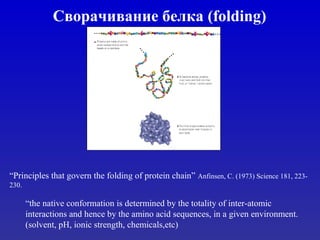
- 1. Сворачивание белка (folding) “Principles that govern the folding of protein chain” Anfinsen, C. (1973) Science 181, 223- 230. “the native conformation is determined by the totality of inter-atomic interactions and hence by the amino acid sequences, in a given environment. (solvent, pH, ionic strength, chemicals,etc)
- 2. Проблема сворачивания белка •Функции белков определяются исключительно их 3D структурой, конформацией •Вопрос: можно ли предсказать 3D структуру белка, исходя из данной аминокислотной последовательности? •Ответ: в общем случае – нет! • Но методы, которые позволяют разрешить частично 3D структуры, бывают полезны.
- 3. Сворачивание – почему это так сложно? • Линейные молекулы белков очень быстро сворачиваются в предопределённые 3D структуры. • Свойства любого белка определяются его 3D структурой. • Белки могут денатурировать под воздействием химических веществ или теплоты, но затем они сворачиваются вновь в исходную структуру. Так почему же так сложно разрешить сворачивание? • Структура белка может быть определена экспериментально (X-Rays or NMR) но эта процедура не всегда возможна и не всегда даёт хорошие результаты. • 3D структура последовательности определяется последовательностью допустимых углов поворота, в которой каждый угол «состоит» из 2-х планарных углов. • Эта проблема может быть решена путём дискретизации (при некоторой потере точности) путём ограничения количества возможных путей достижения каждой из точек (координат атомов).
- 4. Если у вас нет структуры…
- 5. Подходы в предсказании структуры • Предсказание 1D: – вторичные структуры –доступность для растворителя – трансмембранальные спирали • Предскание 2D: – контакты между аминокислотами/нитями бета. • Предсказание 3D: –моделирование гомологов – распознавание фолда (e.g. via threading) – ab initio предсказание (e.g. via молекулярная динамика)
- 6. Задачи • Сравнение всех известных структур друг с другом • Классификация и организация всех известных структур • Поиск общих структурных шаблонов и мотивов • Определение эволюционных расстояний между структурами белков • Докинг – изучение взаимодействия между структурами • Предсказание структур на основе последовательности • Дизайн новых лекарств
- 7. Зачем? • Первый шаг к предсказанию третичной структуры • Один из основных элементов в распознавании фолда (для моделирования далеких в эволюционном плане белков)
- 8. Предсказание вторичной структуры http://www.new-science-press.com/ Table II of Williams, R.W. et al.: Biochimica et Biophysica Acta 1987, 916:200-204.
- 9. – предсказание для каждой аминокислоты в выбранном окне соседних аминокислот (13-21) – скоринг, обучение модели и предсказание 2D структуры (маппирование элемента вторичной структуры на окно) Предсказание вторичной структуры
- 10. Методы I. Chou-Fasman / GOR метод II. Модели нейронных сетей III. Методы «ближайшего соседа»
- 11. Метод Chou-Fasman (1974) • Разработан Chou & Fasman в 1974 -1978 • База – известные 3D структуры глобулярных белков – Частоты аминокислот в α-спиралях – Частоты аминокислот в β-листах – Частоты аминокислот в β-поворотах – Правила образования α-спиралей и β-листов • Основан на растворимых, глобулярных белках – начальная база 15 белков
- 13. Развитие Chou-Fasman 1. Присвоение каждой аминокислоте определенного пула параметров 2. Идентификация a-helix и b-sheet. Удлинение этих областей в обоих направлениях. 3. При перекрытии – сравнение P(H) и P(E) и скоринг.
- 14. 1. Вероятности Pα(H)=[(#H in helix)/(#H)]/(fraction helix {all}) T S P T A E L M R S T G P(H) 69 77 57 69 142 151 121 145 98 77 69 57 P(E) 147 75 55 147 83 37 130 105 93 75 147 75 P(turn) 114 143 152 114 66 74 59 60 95 143 114 156 Развитие Chou-Fasman
- 15. Поиск a-спирали 2. Поиск областей, где 4 из 6 аминокислот имеют P(H) >100 (“ ядро a- спирали”) T S P T A E L M R S T G P(H) 69 77 57 69 142 151 121 145 98 77 69 57 T S P T A E L M R S T G P(H) 69 77 57 69 142 151 121 145 98 77 69 57
- 16. Удлинение ядра a-спирали 3. Расширение области ядра, пока 4 аминокислоты имеют среднее P(H) >100. T S P T A E L M R S T G P(H) 69 77 57 69 142 151 121 145 98 77 69 57
- 17. Поиск β-листа 4. Поиск областей, где 3 из 5 аминокислот имеют P(E) >100 “ядро β-листа” 5. Удлинение ядра до тех пор, пока 4 соседних аминокислоты имеют среднее P(E) > 100 6. Если score области > 105 и среднее P(E) > среднее P(H), значит эта область - β-лист T S P T A E L M R S T G P(H) 69 77 57 69 142 151 121 145 98 77 69 57 P(E) 147 75 55 147 83 37 130 105 93 75 147 75
- 18. GCG Programs • PepPlot – Plot on parallel panels – -cff option, text output • PeptideStructure – text output (Most useful for detail) • PlotStructure – two outputs • squiggles “protein-like” • parallel panels
- 19. GOR III (Garnier-Osguthorpe-Robson. Gibrat J.F., J.Mol.Biol, 1987)
- 20. Модели нейронных сетей - Машинное обучение - Сет структур (e.g. a-спирали, не a-спирали) - Обучение распознавать шаблоны, структуры в известных белках Эффективность ~ 70 –75% Rost B. Sander C. Prediction of Protein Secondary Structure at Better then 70% Accuracy. J.Mol.Biol., 1993, vol. 232. 584-599.NPS@ сервер
- 22. Eva
- 24. Предсказание вторичной структуры Predict Protein (Mega) - secondary structure ( PHDsec, and PROFsec) PSI-pred (PSI-BLAST profiles used for prediction; David Jones, Warwick) PHD - Rost & Sander, EMBL, Germany ASPSSP server Raghava, INDIA DSC - King & Sternberg (this server) PREDATOR - Frischman & Argos (EMBL) ZPRED server Zvelebil et al., Ludwig, U.K. nnPredict Cohen et al., UCSF, USA. BMERC PSA Server Boston University, USA SSP (Nearest-neighbor) Solovyev and Salamov, Baylor College, USA. • JPRED Consensus prediction (Cuff & Barton, EBI) • NPS@
- 27. Предсказание функции Еще одна важная задача протеомики — анализ и предсказание функции белка. Известно, что функция белка определяется его активными сайтами, поэтому накопление и систематизация информации об активных сайтах белков чрезвычайно актуальна. В. Иванисенко, Д. Григоровичем и С. Пинтусом разработана компьютерная база данных PDBSite, которая содержит информацию о более чем 12 тысячах активных сайтов белков. Источником информации служат хорошо документированные пространственные структуры белков.
- 28. • парное выравнивание; • множественное выравнивание; • поиск гомологов, threading; • структурное выравнивание. Основные методы в биоинформатике:
- 29. CASP Critical Assessment of Techniques for Protein Structure Prediction CASP1 (1994) CASP2 CASP3 CASP4 CASP5…..CASP9 (2010) • Comparative modeling (CM) • Fold-recognition (FR) • CAFASP meta-server ver. 3 • New folds (NF) • Ten most wanted sec. struct. contacts, protein-protein docking, and disordered predictions.
- 30. About CASP: CASP is a blind study/experiment that aims at establishing the current state of the art in protein structure prediction; identifying what progress has been made; and highlighting where future effort may be most productively focused (Every two years). This blind study is held over an ~8 month time period and ends in a meeting held every two years, in Asilomar, CA, starting from 1994. For the procedure of the experiment, CASP participants are first provided target sequences (around May) via the Protein Structure Prediction Center at Lawrence Livermore National Laboratory. The participants have a few months to determine the template structure, alignment, model structure and evaluate their results. The sequence targets are categorized by homology and difficulty for predicting their structure. The fairly simple targets have med. sequence homology (>30% seq. identity) are considered comparative modeling (CM) predictions; the med. difficulty targets have med.-to-low sequence homology (~10- 30% seq. identity) are considered fold-recognition (FR) predictions; and the difficult targets have low seq. homology and usually require an ab initio methods are considered new folds (NF). During the prediction time (~May-Oct.), researchers (structural biologist in x-ray or NMR) work on solving the experimental structure of each of the target sequences and they hold back the structure coordinate information from the predictors. By Nov., all participants submit their models (as coordinates) to the Livermore Center and the researchers (who solve the target structure) finalize and post their results. Finally, in Dec., all participants and the CASP organizers meet to evaluate the results of the experiment comparing each model with the experimental structure and discussing the methodologies used. The goal of CAFASP is to evaluate the performance of fully automatic structure prediction servers available to the community. In contrast to the normal CASP procedure, CAFASP aims to answer the question of how well servers do without any intervention of experts, i.e. how well ANY user using only automated methods can predict protein structure. CAFASP assesses the performance of methods without the user intervention allowed in CASP.
- 32. Предсказание сворачивания белка vs предсказание структуры Престказание процесса фолдинга белка связано с процессом приобретения белком его 3D формы, очертаний – физико-химические принципы. Предсказание структуры – используются любые статистические, теоретические и эмпирические данные. 4 подхода: Моделирование гомологов (Homology Modeling) Распознавание фолда (Sequence-Structure Threading (secondary structure prediction)): • Dynamic programming • Knowledge-based potentials Предсказание Ab initio Docking and Drug Design
- 33. • Моделирование гомологов (homology modeling) • Ab initio предсказание • Распознавание сворачивания “Threading'‘ • Докинг Техники фолдинга белка
- 34. Сравнительное моделирование гомологов Для последовательностей с гомологичностью > 25-30% использовать известную PDB структуру как отправной пункт для создания 3D модели структуры неизвестной последовательности. Нужно использовать координаты основной цепи (N-Cα-C) гомологичной структуры как шаблон для модели 70% и более гомологичности – очень высокое качество модели, даже положения боковых цепей могут быть предсказаны с высокой точностью. 40%-65% - средняя точность предсказания. Могут быть серьёзные ошибки даже в положении основной цепи, особенно в областях петельизгибов.
- 35. Лекарственные средства, разработанные с использованием неверных представлений о структуре белка, могут быть токсичны или обладать неучтёнными побочными эффектами. Для эффективности этого метода требуется по меньшей мере 3,000 уникальных, совершенно точно определённых структур. На конец 2001 года имелось только 1,000 уникальных структур среди 16973 в PDB. 2008 год – 53000 структур в PDB, homo sapience ~1500.
- 36. 1. Последовательность-цель – первичная структура белка, 3D структуру которого следует определить 2. Шаблон – белок, чья 3D структура ясна 3. Выравнивание последовательностей 1 и 2 Сравнительное моделирование гомологов Желательно также иметь Биохимическую и структурную информацию (литература) Дополнительные последовательности гомологов с известной структурой
- 37. Моделирование гомологов 1. Fragment-based modeling: Выравнивание с целью идентификации структурно- постоянных областей (SCR): а) области без вставок- делеций и в) области с четко определяемой вторичной структурой. VR – области между SCR. Composer (Sybil), Homology (InsightII) 2. Restraint-based modeling: получение score-функции путём комбинирования «ограничений» - расстояний между Сα, торсионных углов и т.д. Оценка результатов MD данной score- функцией. Modeller
- 38. Swiss-PDBViewer
- 39. • Моделирование гомологов • Предсказание Ab initio • Распознавание сворачивания “Threading'‘ • Докинг
- 40. Предсказание Ab initio Применяется, когда неизвестны гомологи, нет структуры, которую можно было бы использовать как шаблон Есть только одна последовательность. Предсказание 3D основано на «базовых» принципах, таких, как энергетические и статистические законы и правила. Это – симуляция физических сил и процессов, которые могут привести развёрнутый белок в нативную (стабильную, присутствующую в природе) конформацию на компьютере Стабильность с точки зрения термодинамики: нативная конформация белка есть его глобальный минимум свободной энергии. Белок должен сворачиваться так самостоятельно.
- 41. Предсказание Ab initio Электростатические Ван-Дер-Ваальс Водородные связи Энергия торсионных связей
- 42. Предсказание Ab initio - сворачивание Полный расчёт энергий – очень затратный с точки зрения вычислений процесс. Поэтому требуется разработка неких эвристических энергетических функций, которые бы надёжно различали «правильную» и «неправильную» структуры и лучше «понимали» бы силы, которые управляют сворачиванием белка.
- 44. Фолдинг. Предсказание Ab initio Protein Folding: A Perspective from Theory and Experiment Christopher M. Dobson,* Andrej Sœ ali, and Martin Karplus*
- 45. Предсказание Ab initio Сравнение расчётной и экспериментальной модели для белка миоглобина и использованием refined potential function. Рассчитанная структура является 3D структурой, полученной в результате 3-х разных расчётов с дальнейшей кластеризацией и выбором структуры с наименьшей энергией. Общее время симуляции на кластере из 16 машин CM-5 massively parallel computer составило 60 часов, в течении которых было генерировано порядка 5 миллионов структур. RMS составляет 6.2 Å.
- 46. Парадокс Левенталя Время, за которое белок скручивается, (принимает конечное 3D состояние) на много порядков меньше времени перебора всех возможных конфигураций. Допустим, в белке 100 атомов, каждый из которых принимает 3 положения: 3 100 = 5 × 10 47 конформаций. Наибыстрейшее движение – 10- 15 с. Перебор всех конформаций займёт 5 × 10 32 с или 1.6 × 10 25 лет (возраст Вселенной ~ 13,75 × 10⁹ )
- 47. • Homology Modeling • Ab initio prediction • Fold Recognition or “Threading'‘
- 48. Распознавание сворачивания (“Threading”) Напоминает метод моделирования гомологов, но не требует структур с высокой степенью идентичности. Интересующая нас последовательность «протягивается» через все возможные позиции основной цепи во всех известных белковых структурах в PDB, и для каждой итерации рассчитывается её свободная энергия. Структура, которая даст лучший показатель энергии принимается за «шаблон» и дальнейший процесс напоминает моделирование гомологов Threading не может быть применён для тех белков, для которых в базе PDB нет похожих структур.
- 49. Из «Methods in Molecular Biology, vol 143, Methods and ProtocolMethods and Protocols. Protein Structure Prediction, еdited by David M. Webster» Profiles-3D scoring function: оценка локального структурного выравнивания (укладки) каждой аминокислоты в последовательно- сти без учета попарного взаимодей- ствия аминокислот+склонность к H/E/L структурам+полярность (solvent exposure) Распознавание сворачивания (“Threading”)
- 50. Рисунок из R. Lathrop et al, “Analysis and Algorithms for Protein Sequence-Structure Alignment” in Computational Methods in Molecular Biology, Salzberg et al. editors, 1998. Распознавание сворачивания (“Threading”)
- 51. Fold Recognition – The Fold PDB Groups clustered by a common resemblanc e Genome Sequencing Homology Structure Conservation Calculated Folds Сколько всего фолдов? Количество фолдов ~ 4000 БД из 930 фолдов ~ 90% семейств белков
- 52. Fold Recognition – недостатки Этот метод редко приводит к тому качеству структурного выравнивания, которое предоставляет моделирование гомологов.
- 53. Серверы •PredictProtein Server •ModBase (a database of three-dimensional protein models calculated by comparative modeling( 3D PSSM & ModBase 3D-PSSM предсказание 3D структуры по последовательности и вероятность этой структуры ModBase – база данных 3D структур, построенных на основе сравнительного моделирования
Notas do Editor
- 1
- Experimental data can aid the structure prediction process. Some of these are: Disulphide bonds, which provide tight restraints on the location of cysteines in space Spectroscopic data, which can give you and idea as to the secondary structure content of your protein Site directed mutagenesis studies, which can give insights as to residues involved in active or binding sites Knowledge of proteolytic cleavage sites, post-translational modifictions, such as phosphorylation or glycosylation can suggest residues that must be accessible Protein Sequence: Transmembrane? Coil-coil? Does your protein contain regions of low complexity? Proteins frequently contain runs of poly-glutamine or poly-serine, which do not predict well (SEG program). If the answer to any of the above questions is yes, then it is worthwhile trying to break your sequence into pieces, or ignore particular sections of the sequence, etc. This is related to the problem of locating domains .
- Fig.:Coverage for each species is reported as the fraction of the residues in the proteome that are annotated . Structural annotation is an homology to a known structure. Functional annotation is when there is no structural annotation but there is an homology to a sequence database entry that has a useful description. Homology denotes a sequence similarity to a structurally or functionally un-annotated protein, such as one described as hypothetical. Non-globular denotes remaining sequence regions that were predicted as transmembrane, signal peptide, coiled-coils or low-complexity. Remaining residues are classified as orphans.
- Analysis of the frequency with which different amino acids are found in different types of secondary structure shows some general preferences. For example, long side chains such as those of leucine, methionine, glutamine and glutatamic acid are often found in helices, presumably because these extended side chains can project out away from the crowded central region of the helical cylinder. In contrast, residues whose side chains are branched at the beta carbon , such as valine, isoleucine and phenylalanine are more often found in beta sheets, because every other side chain in a sheet is pointing in the opposite direction, leaving room for beta-branched side chains to pack. Such tendencies underlie various empirical rules for the prediction of secondary structure from sequence, such as those of Chou and Fasman. In the Chou-Fasman and other statistical methods of predicting secondary structure, the assumption is made that local effects predominate in determining whether a stretch of sequence will be helical, form a turn, compose a beta strand, or adopt an irregular conformation. This assumption is probably only partially valid, which may account for the failure of such methods to achieve close to 100% success in secondary structure prediction. The methods take proteins of known three-dimensional structure and tabulate the preferences of individual amino acids for various structural elements. By comparing these values with what might be expected randomly, conformational preferences can be assigned to each amino acid. To apply these preferences to a sequence of unknown structure, a moving window of about five residues is scanned along a sequence, and the average preferences are tallied. Empirical rules are then applied to assign secondary structural features based on the average preferences. Unfortunately, these tendencies are only very rough, and there are many exceptions. It is probably more useful to consider which side chains are disfavored in particular types of secondary structures. With specialized exceptions Proline is disfavored in both helices and sheets because it has no backbone N-H group to participate in hydrogen bonding. Glycine is also less commonly found in helices and sheets, in part because it lacks a side chain and therefore can adopt a much wider range of phi, psi torsion angles in peptides. These two residues are, however, strongly associated with beta turns, and sequences such as Pro-Gly and Gly-Pro are sometimes considered diagnostic for turns. Although predictive schemes based on residue preferences have some value, none is completely accurate, and the one rule that seems to be most reliable is that any amino acid can be found in any type of secondary structure, if only infrequently. Proline, for instance, is sometimes found in alpha helices; when it is, it simply interrupts the helical hydrogen-bonding network and produces a kink in the helix.
- 1974 Chou and Fasman propose a statistical method based on the propensities of amino acids to adopt secondary structures based on the observation of their location in 15 protein structures determined by X-ray diffraction. Clearly these statistics derive from the particular stereochemical and physicochemical properties of the amino acids. See for example, glycine and proline. These statistics have been refined over the years by a number of authors (including Chou and Fasman themselves) using a larger set of proteins. Rather than a position by position analysis the propensity of a position is calculated using an average over 5 or 6 residues surrounding each position. On a larger set of 62 proteins the base method reports a success rate of 50%. 1978 Garnier improved the method by using statistically significant pair-wise interactions as a determinant of the statistical significance. This improved the success rate to 62% 1993 Levin improved the prediction level by using multiple sequence alignments. The reasoning is as follows. Conserved regions in a multiple sequence alignment provides a strong evolutionary indicator of a role in the function of the protein. Those regions are also likely to have conserved structure, including secondary structure and strengthen the prediction by their joint propensities. This improved the success rate to 69%. 1994 Rost and Sander combined neural networks with multiple sequence alignments. The idea of a neural net is to create a complex network of interconnected nodes, where progress from one node to the next depends on satisfying a weighted function that has been derived by training the net with data of known results, in this case protein sequences with known secondary structures. The success rate is 72%.
- Simulate the brain. Selection of training sets is extremely important. Different protein families, only one or two representative from each family.
- Jpred: (http://www.dl.ac.uk/CCP/CCP11/newsletter/vol2_4/jpred_ccp11/) Jpred runs DSC (5), PHD (1,2), PREDATOR (3,4) and NNSSP (6) in parallel to build its consensus prediction, but predictions from slightly less accurate algorithms MULPRED (8) and ZPRED (7) are also included in the final output. These methods were chosen as representatives of current state-of-the-art secondary structure predictions methods that exploit the evolutionary information from multiple sequences. Each derives its prediction using a different heuristic, based upon nearest neighbours (NNSSP), jury decision neural networks (PHD), linear discrimination (DSC), consensus single sequence method (MULPRED), hydrogen bonding propensities (PREDATOR), or conservation number weighted prediction (ZPRED). The consensus is constructed using a simple majority wins combination of DSC, PHD, PREDATOR and NNSSP, relying on the PHD prediction if there is a a tie. In our study, we found this combination to be optimal.
- Flowchart of EVA. Every day, EVA downloads the newest protein structures from PDB [1] . The structures are added to mySQL databases, sequences are extracted for every protein chain, and are sent to each prediction server by META-PredictProtein [2] . META-PP collects the results and sends them to EVA. Every week, EVA runs alignment programs for searching sequence (iterated PSI-BLAST [3] , MaxHom [4] ) and structure (CE [5] , ProSub [6] ) databases to determine homologues. Predictions of secondary structure and inter-residue contacts, as well as, comparative modelling are evaluated at the EVA satellites at Columbia University, Rockefeller University, and CNB Madrid. Goals: CASP addresses the question ‘how well can experts predict protein structure if given sufficient incentive to do so?’. In contrast, the question addressed by EVA is ‘how well could molecular biologists predict protein structure, if they simply take the output from the programs out there?’. Thus, the goals are: Provide a continuous, fully automated, and statistically significant analysis of structure prediction servers. As has been shown by many of us, predictions based on small numbers of samples are NOT representative. EVA running for a year could produce a fairly representative picture. Even running for a month EVA could produce more reliable estimates than CASP can do in 2 years (at least, for answering the particular, restricted — but important - question ‘how well do servers do’). EVA will NOT answer to requests of users!! It will NOT be a meta-server, rather it will simply sit there and evaluate servers based on known structures. EVA will NOT evaluate any server without the consent of the author.
- SSE – secondary structure elements Perutz (1990) showed (while working with hemoglobin and myoglobin) that amphipathicity can be detected in the sequnce: non polar residues can appears every 3.6 approx. in a linear sequence, making one side of the helix hydrophobic.
- An example of the prediction of secondary structure from sequence for a protein of unknown function from the Enterococcus faecalis genome. What is striking is that all of the schemes agree on the approximate locations of the alpha helices (h) and beta strands (e), but they disagree considerably on the lengths and end positions of these segments. Note also that the probable positions of loops (indicated by a c) and turns (indicated by a t) are very inconsistently predicted. Such results are typical, but the application of many methods is clearly more informative than the use of a single one. The bottom line shows the consensus prediction.
- The upper one is by Jpred and the lower one is by GOR
- 1wqa, 1tx4, 1grn, 1tad and 1gfi. -> only 1tx4, 1grn, 1tad Note that some amino acids may appear in yellow once a molecule has been loaded. It signifies that their sidechain has been reconstructed during the loading process because some atoms were lacking. When all sidechain atoms are lacking, a rotamer library is searched until the rotamer that generate a maximum of H-bonds and a minimum of steric hindrances is found. If only some sidechain atoms are lacking, the rotamer that gives the lowest RMS when fitted to the partial sidechain is taken. In any case, you may try to find a better sidechain manually with the mutation tool. If you want to act on a complete column , simply hold down the shift key while clicking in a column Note: if a little earth icon is shown below the first tool, the rotation takes place in absolute coordinates. Otherwise (little protein icon) molecules are rotated around their centrotid. Hence the first option allows you to rotate the molecule around any atom, providing that this atom has previously been centered (translated to the (0,0,0) coordinate). Note: if "caps lock" is down, you can measure several distances or angles successively. To exit the "repeated" measurement mode, you can either depress "caps lock" or hit "esc".
- Устные пояснения.