crypto info

1. The Economics of Cryptocurrencies
– Bitcoin and Beyond∗
Jonathan Chiu†
Bank of Canada
Thorsten V. Koeppl‡
Queen’s University
First version: March, 2017
This version: September, 2018
Abstract
How well can a cryptocurrency serve as a means of payment? We study the optimal design of
cryptocurrencies and assess quantitatively how well such currencies can support bilateral trade.
The challenge for cryptocurrencies is to overcome double-spending by relying on competition
to update the blockchain (costly mining) and by delaying settlement. We estimate that the
current Bitcoin scheme generates a large welfare loss of 1.4% of consumption. This welfare loss
can be lowered substantially to 0.08% by adopting an optimal design that reduces mining and
relies exclusively on money growth rather than transaction fees to finance mining rewards. We
also point out that cryptocurrencies can potentially challenge retail payment systems provided
scaling limitations can be addressed.
Keywords: Cryptocurrency, Blockchain, Bitcoin, Double Spending, Payment Systems
JEL Classification: E4, E5, L5
∗
The views expressed in this paper are not necessarily the views of the Bank of Canada. We thank the audiences
at many seminars and conferences for their comments. This research was supported by SSHRC Insight Grant 435-
2014-1416. The authors declare that they have no relevant or material financial interests that relate to the research
described in this paper.
†
Bank of Canada, 234 Wellington St, Ottawa, ON K1A 0H9, Canada (e-mail: jchiu@bankofcanada.ca).
‡
Queen’s University, Department of Economics, Kingston, K7L 3N6, Canada (e-mail: thor@econ.queensu.ca).
1

2. 1 Introduction
How well can a cryptocurrency serve as a means of payment? Since the creation of Bitcoin in 2009,
many critics have denounced cryptocurrencies as fraud or outright bubbles. More nuanced opinions
have argued that such currencies are only there to support payments for illegal activities or simply
waste resources. Advocates point out, however, that – based on cryptographic principles to ensure
security – these new currencies can support payments without the need to designate a third-party
that controls the currency or payment instrument possibly for its own profit.1
We take up this discussion and develop a general equilibrium model of a cryptocurrency that
uses a blockchain as a record-keeping device for payments. Although Bitcoin in its current form
has immense welfare costs, an optimally designed cryptocurrency can potentially support payments
rather well. First, using Bitcoin transactions data, we show that the welfare cost of a cryptocurrency
can be comparable to a cash system with moderate inflation. Second, using summary statistics for
US debit card transactions, we find that a cryptocurrency can perform nearly as well as a low-value,
retail payment system operating with very low fees.2
Economics research so far has provided little insight into the economic relevance of cryptocurrencies.
Most existing models of cryptocurrencies are built by computer scientists who mainly focus on the
feasibility and security of these systems. Crucial issues such as the incentives of participants to
cheat and the endogenous nature of some key variables such as the real value of a cryptocurrency
in exchange have been largely ignored. Such considerations, however, are pivotal for understanding
the optimal design and, hence, the economic value of cryptocurrency as a means of payment.
Our focus is primarily on understanding how the design of a cryptocurrency influences the inter-
actions among participants and their incentives to cheat. These incentives arise from a so-called
“double-spending” problem. Cryptocurrencies are based on digitial records and, thus, can be copied
easily and costlessly which means that they can potentially be used several times in transactions
1
Some central banks have recently started to also explore the adoption of cryptocurrency and blockchain technolo-
gies for retail and large-value payments. Examples are the People’s Bank of China who aims to develop a nationwide
digital currency based on blockchain technology; the Bank of Canada and the Monetary Authority of Singapore who
are studying its usage for interbank payment systems; and the Deutsche Bundesbank who has developed a preliminary
prototype for blockchain-based settlement of financial assets.
2
This raises the issue that many cryptocurrencies currently cannot be scaled sufficiently to function as a true
replacement of large retail payment networks. We abstract completely from such scalability issues that mainly arise
from technological constraints.
2

3. (for a more detailed description see Section 2 below). We formalize this double-spending problem
and show how this problem is being addressed by (i) a resource-intensive competition for updating
the records of transaction – a process commonly referred to as mining – and (ii) by introducing con-
firmation lags for settling transactions in cryptocurrency. This implies that a cryptocurrency faces
a trade-off between how fast transactions settle and a guarantee (or “finality”) for their settlement.
Consequently, crytocurrencies cannot achieve immediate and final settlement of transactions.
A strength of our analysis is that we take into account the costs of operating a cryptocurrency
that prohibits double-spending. This allows us to quantitatively assess how efficient Bitcoin as a
medium of exchange can be relative to existing means of payment. Calibrating our model to Bitcoin
data, we find that from a social welfare perspective using Bitcoin is close to 500 times more costly
than using traditional currency in a low inflation environment.
This is, however, a result of the inefficient design of Bitcoin as a cryptocurrency. Bitcoin uses
both currency growth and transaction fees to generate rewards for mining. In its current form, the
cryptocurrency reward structure is too generous so that too many resources are being used to rule
out double-spending and making it a secure form of payment. We show that the optimal way of
providing rewards for mining is exclusively via currency creation at a very low rate rather than by
using transaction fees. The optimal design of Bitcoin would generate a welfare cost of only about
0.08% of consumption which is equivalent to a cash system with moderate inflation.
We also evaluate the efficiency of using a cryptocurrency system to support large-value and retail
transactions. Using summary data for Fedwire and US Debit cards, we confirm that cryptocur-
rencies are a much better alternative for low value, high-volume transactions than for large value
payments. This is intuitive, as double spending incentives increase with the size of transactions.
Hence, more mining and longer confirmation lags (which are both costly) are required when sup-
porting large-value payments in a cryptocurrency. Our exercise shows that cryptocurrency systems
can potentially be a valid alternative to retail payment systems that operate at very low fees, as
soon as limits on the scale of such systems can be resolved.
The economic literature on cryptocurrencies is very thin. We are not aware of any work that
has formalized the design features of a cryptocurrency and that has studied its optimal design
under the threat of double spending attacks. We model bilateral exchange based on money, we
follow the recently promoted framework of Lagos and Wright (2005) and enrich it by modelling a
mining competition to update the blockchain. For formalizing the blockchain itself, we rely on the
3

4. theoretical literature of payment systems as a record-keeping device.3
Our work is thus a first attempt to explicitly model the distinctive technological features of a
cryptocurrency system which are a blockchain, mining and double-spending incentives within a
quantitative economic model. We are also first to theoretically analyze the optimal design of a
cryptocurrency and giving a quantitative answer to the efficiency properties of cryptocurrencies.
Some recent contribution have analyzed – from a qualitative perspective – whether Bitcoin can
function as a real currency given its security features and lack of usage for making frequent payments
(see for example Yermack (2013) and Böhme et al. (2015)). One question in this line of research
is to empirically explain the valuation of cryptocurrencies. Gandal and Halaburda (2014) look at
network effects associated with cryptocurrencies and investigate how such effects are reflected in
their relative valuation. Glaser et al. (2014) look at how media coverage of Bitcoin drives part of
the volatility in its valuation.4
Another area of research investigates how digital currencies can influence the way monetary policy is
conducted. But none of this work can be applied to cryptocurrencies that are based on a blockchain
and operate without a designated third-party to issue the currency. Agarwal and Kimball (2015)
advocate here that the adoption of digital currencies can facilitate the implementation of a negative
interest rate policy, while Rogoff (2016) suggests that phasing out paper currency can undercut
undesirable tax evasion and criminal activities. Our findings complements this work as we establish
some potential bounds on the costs that can be levied on people through central bank issued
digital currency.5 Finally, Fernández-Villaverde and Sanches (2016) model cryptocurrencies as
privately issued fiat currencies and analyze – in the tradition of the literature on the free banking
era – whether competition among different currencies can achieve price stability and efficiency of
exchange.
3
See for example Koeppl et al. (2008) and (2012).
4
Models have been developed for studying other forms of electronic money technologies. For example, Berentsen
(1998) studies digital money such as smart cards; Gans and Halaburda (2013) study platform-specific digital currencies
such as Facebook Credits; Chiu and Wong (2015) review e-money technologies including PayPal and Octopus Card.
5
See the recent discussion of Bordo and Levin (2017) on central bank issued digital currency. Also, Camera (2017)
reviews the monetary literature and discusses the challenges of issuing and adopting electronic alternatives to cash.
4

5. 2 Cryptocurrencies: A Brief Introduction
Our modern economy relies heavily on digital means of payments. Trade in the form of e-commerce
for example necessitates the usage of digital tokens. In a digital currency system, the means of
payment is simply a string of bits. This poses a problem, as these strings of bits as any other
digital record can easily be copied and re-used for payment. Essentially, the digital token can be
counterfeited by using it twice which is the so-called double-spending problem.
Traditionally, this problem has been overcome by relying on a trusted third-party who manages
for a fee a centralized ledger and transfers balances by crediting and debiting buyers and sellers’
accounts. This third-party is often the issuer of the digital currency itself, one prominent example
being PayPal, and the value of the currency derives from the fact that users trust the third-party
to prohibit double-spending (top of Figure 2.1).
Cryptocurrencies such as Bitcoin go a step further and remove the need for a trusted third-party.
Instead, they rely on a decentralized network of (possibly anonymous) validators to maintain and
update copies of the ledger (bottom of Figure 2.1). This necessitates that consensus between the
validators is maintained about the correct record of transactions so that the users can be sure to
receive and keep ownership of balances. But such a consensus ultimately requires that (i) users do
not double-spend the currency and (ii) that users can trust the validators to accurately update the
ledger.
How do cryptocurrencies such as Bitcoin tackle these challenges? Trust in the currency is based
on a blockchain which ensures the distributed verification, updating and storage of the record of
transaction histories.6 This is done by forming a blockchain. A block is a set of transactions
that have been conducted between the users of the cryptocurrency. A chain is created from these
blocks containing the history of past transactions that allows one to create a ledger where one
can publicly verify the amount of balances or currency a user owns. Hence, a blockchain is like a
book containing the ledger of all past transactions with a block being a new page recording all the
current transactions.
Figure 2.2 illustrates how the blockchain is updated. To ensure consensus, validators compete for
6
In this sense it is different from traditional money which is merely a partial memory of past transactions as it
only records the current distribution of balances and does not record how past transactions generate the current
distribution.
5

6.
Digital tokens with a trusted third party (e.g. PayPal)
Digital tokens without a trusted third party (e.g. Bitcoin)
Figure 2.1: Digital Currency vs. Cryptocurrency
6

7.
Figure 2.2: Blockchain Based Validation in a Cryptocurrency
the right to update the chain with a new block. This competition can take various forms. In Bitcoin,
it happens through a process called mining. Miners (i.e. transaction validators) compete to solve
a computationally costly problem which is called proof-of-work (PoW).7 The winner of this mining
process has the right to update the chain with a new block. The consensus protocol prescribes
then that the “longest” history will be accepted as the trusted public record.8 Since transaction
validation and mining are costly, a reward structure is needed for mining to take place. In Bitcoin,
for example such rewards are currently financed by the creation of new coins and transaction fees.9
The main concern for users when trusting a cryptocurrency is the double spending problem: after
having conducted a transaction, a user attempts to convince the validators (and, hence, the general
public if the blockchain is trusted) to accept an alternative history in which some payment was
not conducted.10 If this attack succeeds, this user will keep both the balances and the product
7
Other consensus protocols are being explored which we briefly discuss in the Appendix.
8
In general, there is no explicit requirement to follow the consensus protocol in the sense that validators and users
can trust an alternative history or blockchain that is not the longest one. Well-designed cryptocurrency, however,
try to ensure that there are sufficient incentives to work with the longest history. For example, in Bitcoin the reward
paid to a successful miner is contained in the new block itself. Should a different chain be adopted at a later stage,
this reward will be obsolete. For a game-theoretic analysis of the incentives to build on the longest chain, see Biais
et. al. (2017).
9
Huberman et al. (2017) explore the reward structure of cryptocurrencies from the perspective of the mining
game, but without modelling the double spending problem.
10
While basic cryptography ensures that people cannot spend others’ balances, a miner can exclude from a block
7

8. or service he obtained while the counterparty will be left empty handed. Hence, the possibility of
such double-spending can undermine the trust in the cryptocurrency.
A blockchain based on a PoW consensus protocol naturally deals with changing transaction history
backwards. The blockchain has to be dynamically consistent in the sense that current transactions
have to be linked to transactions in all previous blocks.11 Consequently, if a person attempts to
revoke a transaction in the past, he has to propose an alternative blockchain (with that particular
transaction removed) and perform the PoW for each of the newly proposed block. Therefore, it is
very costly to rewrite the history of transactions backwards if the part of the chain that needs to
be replaced is long. Hence, the “older” transactions are, the more users can trust them.
Unfortunately, a blockchain does not automatically protect a cryptocurrency against a double-
spending attack that is forward-looking. Figure 2.3 considers a spot trade between a buyer and
a seller involving a cryptocurrency. The buyer instructs the miners to transfer a payment to the
seller while the seller simultaneously delivers the goods. Notice that the buyer can always secretly
mine an alternative history (or submit to some miners a different history) in which the fund is
not transferred. The final outcome of the transaction depends on which payment instruction is
incorporated into the blockchain first. If the former payment instruction is incorporated, then the
double-spending attempt fails. The seller receives the payment and the buyer gets the goods. If
the latter is accepted instead, then the double-spending attempt succeeds. In this case, the buyer
gets the goods without paying the seller.
Such a double spending attack can be discouraged by introducing a confirmation lag into the
transactions. By waiting some blocks before completing the transaction (i.e., the seller delays the
delivery of the goods), it becomes harder to alter transactions in a sequence of new blocks. Figure
2.4 illustrates how a confirmation lag of one block confirmation raises the secret mining burden of
a double spender. The seller delivers the goods only after the payment is incorporated into the
blockchain at least in one new block. Again, the buyer can secretly mine an alternative history
in which the payment does not happen. How successful secret mining is depends on the mining
competition and the length of the confirmation lag.
some transactions that have been initiated by other people. With positive transaction fees, a miner does not have an
incentive to remove other people’s transactions and lose such fees.
11
For example, if someone transfers a balance d in block T, it must be the case that the person has received
sufficient net flows from block 0 to block T − 1 so that the accumulated amount is at least d.
8

9. Double spending attempt fails
Double spending attempt succeeds
Figure 2.3: Double Spending Attack
9

10. Suppose the buyer successfully solves the PoW for the block containing this alternative history.
Note that the buyer has an option whether to broadcast the secretly mined block immediately or
withhold it for future mining. If he decides to broadcast the block immediately, the seller will not
receive the payment, but he will also not deliver the goods as shown on the top of the figure. Hence,
the double-spending attack is not successful for the buyer.
Alternatively, the buyer can temporarily withhold the solved block and continue to secretly mine
another block (depicted on the bottom of the figure). Specifically, the buyer needs to allow other
miners to confirm the original payment to the seller, so as to induce the seller to deliver the goods.
At the same time, the buyer needs to secretly mine two blocks in a row for which the original
transaction is removed.12 If the buyer is successful in mining two blocks faster than other miners,
he can announce an alternative blockchain after the goods are delivered. In this case, the buyer
gets the goods without paying the seller. More generally, if the seller delivers the goods only after
observing N confirmations of the payment, the buyer needs to solve blocks N +1 consecutive times
in order to double spend successfully.
To summarize, trust in a cryptocurrency system involves the interplay of three ideas: the security
of the blockchain, the health of the mining ecosystem and the value of the currency.13 As shown
in Figure 2.5, sufficient mining activities are required for ensuring the security of the blockchain,
safeguarding it against attacks and dishonest behaviors. Moreover, only when users trust the
security of system will the cryptocurrency be widely accepted and and traded at a high value.
Finally, the value of the currency supports the reward scheme to incentivize miners to engage in
costly mining activities.
Our model will capture precisely this interdependence by explicitly looking at the joint determina-
tion of mining efforts, rewards and cryptocurrency value in general equilibrium. The main features
of a cryptocurrency model in Section 3 are therefore given by
(i) a consensus protocol: miners compete to update a blockchain with the probability of winning
being proportional to the fraction of computational power owned by a miner
12
Since the consensus protocol prescribes that the longest chain is accepted by the miners, the double spender
needs to mine two blocks in order to create an alternative, longer blockchain superseding the existing one which has
one block solved already.
13
This has been pointed out already in the computer science literature (see for example Narayanan et al. (2016)),
but without making the connection to an equilibrium incentive problem for double spending.
10

11. Double spending attempt fails (with one confirmation lag)
Double spending attempt succeeds (with one confirmation lag)
Figure 2.4: Double Spending Attack when Confirmation Lag
11

12. Security of
blockchain
Value of
currency
Mining
activities
merchants willing to
accept currency
reward scheme
make double
spending costly
Figure 2.5: Bootstrapping in a Cryptocurrency System
(ii) settlement lags: double spending is discouraged by sellers waiting for N validations before
delivering the goods so that the buyer needs to win the mining game N + 1 times in order to
revoke a payment
(iii) a reward scheme: rewards for winning miners are financed by seigniorage (new coins) and
transaction fees.
3 The Double Spending Problem
As pointed out in the previous section, due to its digital nature, a cryptocurrency system is subject
to the double spending problem. To focus on this problem, this section develops a partial equilib-
rium model to study the mining and double-spending decision within one payment cycle. Taking
as given the price and quantity of balances, the terms of trade and the mining rewards, this basic
model determines the mining activities and the buyers’ incentives to double spend. In the next
section, we will incorporate this basic set-up into a general equilibrium monetary model to perform
a full analysis.
12

13. 3.1 Basic Set-up
We begin our analysis by looking at a single transaction period. As shown in Figure 3.1, there are
N̄ + 1 subperiods within the single period. In subperiod 0, a buyer meets a seller to negotiate a
trade. All other subperiods 1, . . . , N̄ serve as periods for confirming and settling trades that take
place in subperiod 0.
n = 0 n = 1 n = 2 ... n = N̄
buyer sends d
seller
n = N
double
buyer
spends
delivers x
negotiate (x, d, N)
...
Figure 3.1: Timeline for a single transaction period
The buyer carries a real balance of cryptocurrency equal to z that can be used to buy an amount of
goods x from a seller. Upon being matched, the buyer and the seller bargain to determine the terms
of trade (x, d, N) which specify that the buyer pays the seller d ≤ z units of real balances and that
the seller commits to deliver x units of goods after a number of successive payment confirmations
N ∈ {0, . . . , N̄} in the Blockchain.14 We call N the confirmation lag of the transaction. For now,
the terms of trade are taken as given, but will be determined endogenously in the next section.
The seller produces the good at unit costs, while the buyer’s preference for consuming an amount
x with confirmation lag N are given by
δN
u(x) (1)
where δ ∈ (0, 1) is the discount factor between two subperiods. Hence, discounting across the whole
transaction period is given by15
β = δN̄+1
. (2)
Finally, both buyers and sellers value real balances linearly and discount all payoffs that arise after
the single transaction period at β.
14
We consider the case in which a seller can commit to deliver the good. If this were not the case, only spot trades
can be conducted that – as we show later – will always be subject to double spending.
15
There are two ways to interpret the discount factor δ: (i) buyers prefer earlier consumption or (ii) a buyer’s
preference can change over time so that a seller’s goods will no longer generate utility with probability 1 − δ.
13

14. 3.2 Mining
There are also M miners who compete for updating a blockchain in subperiods n = 0, ..., N̄ with all
the transactions from subperiod 0. In each subperiod, miners perform exactly one costly computa-
tional task with a random success rate by investing computing power, q, measured in real balances
of cryptocurrency.16 This task is called the Proof-of-Work (PoW). We assume that miners value
real balances linearly.
As motivated by the Bitcoin protocol (see Property (i) in Section 2), if the computational power
of miner i in a subperiod is q(i), then the probability that a particular miner i will win the mining
game is given by
ρ(i) =
q(i)
PM
m=1 q(m)
. (3)
In other words, the probability of wining is proportional to the fraction of computational power
owned. We take this feature as given here and provide a micro foundation for this result in the
Appendix. By winning the competition in any subperiod, a miner can update the Blockchain (i.e.,
append the nth block to the Blockchain) and receive a reward R in real balances. We assume that
miners receive and consume this reward after the period, discounted by the time preference β.
Note that the mining games are independent across subperiods. Hence, in any subperiod miner i
solves
max
q(i)
ρiβR − q(i) (4)
so that PM
m=1 q(m) − q∗(i)
P
i6=j q(m) + q∗(i)
2 βR = 1. (5)
where he takes as given the choice by all miners m 6= i. Imposing symmetry, q(m) = Q for all m,
we obtain as the Nash equilibrium of the mining game that
Q =
M − 1
M2
βR. (6)
Consequently, the total computing cost of mining in any subperiod is
MQ =
M − 1
M
βR (7)
16
One could assume that miners buy computing power q at price α so that z units of real balances yield computing
power q = αz. We can, however, simply normalize α = 1 by changing the unit for q.
14

15. The expected profit of a miner in equilibrium across the single transaction period is thus given by
Πm = (N̄ + 1)
Q
PM
m=1 Q
βR − Q
#
=
N̄ + 1
M2
βR. (8)
To capture the fact that mining tends to be quite competitive and open to new entrants, we let
M → ∞17 to arrive at the following lemma.
Lemma 1. As M → ∞, the expected value of miners is zero, and the aggregate computing power
of miners dissipates all rewards from mining
MQ = βR.
3.3 Secret Mining
As discussed in Section 2, an important concern in a cryptocurrency system is a buyer’s double
spending attempts (see Property (ii) in Section 2). When trading, the buyer needs to make a
payment d to the seller. To do so, he has to send out an instruction to miners to update the
Blockchain with the transaction. However, this is insufficient to ensure that the seller receives a
payment. A buyer can engage in secret mining by attempting to mine a block in which his payment
did not occur.18 A seller can protect himself from not receiving the payment by waiting to deliver
the goods until the payment has been incorporated into the blockchain.
Such confirmation of the payment in the Blockchain however may still be not enough. A buyer
can secretly mine a different Blockchain which could be released some periods after the seller has
delivered the good replacing the original Blockchain.19 When such secret mining succeeds, the
17
The total number of miners is estimated to be within the range of 5000 to 100,000 (https://goo.gl/TPFBvA). In
addition, according to blockchain.info, there are altogether 14 mining pools that individually can account for at least
1% of the total hashrate. Finally, it is feasible for miners to use their existing mining capacities to mine different
cryptocurrencies. For example, ASICs (Application-specific integrated circuits) manufactured for Bitcoin can be used
to mine altcoins that use SHA-256 as the hashing algorithm (e.g., Namecoin and Peercoin).
18
The secret mining can be done either by the buyer himself or by hiring a miner to mine a block with the instruction
that the payment did not occur.
19
Notice that, with such secret mining, the buyer cannot spend the balances of any other agent because, to spend
other agents’ balances, one would need to obtain the digital signature of other agents. He can only (i) change the
payment instructions of his own transaction and (ii) remove other payment instructions from being mined – and,
hence, confirmed – in the block. Hence, in reality a buyer trying to double spend has to remove his own payment
and all other payment instructions involving his original balance being spent.
15

16. buyer keeps his original balances and the goods while the seller will be left empty handed. In
response, the seller can choose to postpone the delivery of the goods and wait for N confirmations.
This confirmation lag can potentially deter double spending by the buyer. The idea is that, to undo
a transaction with a confirmation lag of N subperiods, a dishonest buyer needs to win the mining
game N + 1 times in a row. As the number of lags increases, the total PoW required to revoke
a transfer is increasing, making it more costly for a buyer to double spend. Furthermore, secret
mining is deterred by miners’ investments in computing power MQ which, according to Lemma
1, is increasing in the reward R. We look next into the incentives to double spend and call an
offer (x, d, N) double spending proof (DS-proof) if the buyer has no incentive to engage in double
spending in subperiod 0 after the acceptance of the offer.
3.4 Double Spending Proof Contracts
Consider then a trade with the terms (x, d, N). The buyer will receive the goods in subperiod N
when exactly N confirmations of the payment d have been observed in the Blockchain. To double
spend, a buyer can secretly mine an alternative history to undo his payment after he has received
the goods. This implies that the double spender needs to be the first one who solves the PoW
problem for N + 1 consecutive subperiods; i.e., from subperiod 0 to subperiod N. For each of the
first N subperiods, the buyer does not broadcast the new block immediately, so that some other
miners will update the Blockchain and confirm his payment to the seller. The buyer broadcasts his
secretly mined blockchain only after he receives the goods and solves the N + 1th block. When the
double spending attack succeeds, the original payment is cancelled and the N + 1 rewards will be
given to the buyer (see Figure 3.2).
Note first that the quantity of good x being exchanged does not directly matter for a double
spending attack, as it neither changes the payoffs, nor the incentives to engage in an attack. We
consider first subperiod N where the seller delivers his goods. Conditional on having been successful
N times with secret mining20, a buyer can now double spend if successful with mining a new block
in subperiod N. His expected payoff from investing qN is given by
ρ(qN )β[d + (N + 1)R] − qN . (9)
20
We implicitly assume here that once a buyer starts a double spending attack, he does not stop after wining a
block before subperiod N. As shown in the Appendix, this is without loss of generality because, if a buyer decides
to double spend, it is not optimal to quit after winning some consecutive blocks before subperiod N.
16

17. n = 0 n = 1 n = 2 ... ... n = N
(z, 0)
n = N̄
start with
(x, d, N)
agree
buyer
buyer chooses q0
secret mining fails (z − d, d)
buyer chooses q1
secret mining fails (z − d, d)
succeeds
buyer chooses q2
secret mining fails (z − d, d)
succeeds
buyer
chooses qN
secret mining fails
succeeds
(z − d, d)
(z, 0)
succeeds
|
{z
}
Double
Spending
Problem
... ...
buyer and seller
2
Figure 3.2: The Double Spending Problem
The first term captures the expected revenue from double spending. Conditional on having solved
N blocks, with probability
ρ(qN ) =
qN
QM + qN
(10)
the buyer wins the competition again in the N + 1th round, so that he can double spend. The
revenue from double spending is given by the original payment in subperiod 0 which is d. Also,
the buyer obtains the rewards from all new blocks in his chain of length N + 1. The value in real
balances at the end of the period is thus given by β(d + R(N + 1)).
We work now backwards to derive a condition for offers to preclude double-spending. Define
∆ =
d
R
+ (N + 1)
. (11)
As M → ∞, the buyer’s optimal choice with respect to investment in computing power in subperiod
N is then given by
q̂N (d, N) =
p
QMβR∆ − QM = βR
h√
∆ − 1
i
(12)
so that the probability of successful double spending in subperiod N is
ρ(qN ) =
q̂N
QM + q̂N
=
√
∆ − 1
√
∆
. (13)
17

18. To derive the no-double-spending constraint we work backwards. Given (d, N) and R, the expected
payoff for a double spending buyer in subperiod N having been successful N times already is
DN (d, N) = βR(
√
∆ − 1)2
. (14)
Define recursively the expected payoff from double spending in subperiod n for n ∈ {0, . . . , N − 1}
by
Dn(d, N) = max
qn
ρ(qn)Dn+1(d, N) − qn, (15)
which takes into account that the buyer was n times successful, since if he fails once the double
spend fails as well. Note that Dn(d, N) can only be positive if Dn+1(d, N) is positive and q̂n 0
only if Dn(d, N) 0. The first-order condition describing the optimal investment is thus given by
q̂n(d, N) =
p
QM · Dn+1(d, N) − QM. (16)
By backward induction, we then obtain the following result.
Lemma 2. As M → ∞,
DN−s(d, N) = βR
h√
∆ − (s + 1)
i2
, (17)
ρN−s(d, N) =
√
∆ − (s + 1)
√
∆ − s
, (18)
q̂N−s(d, N) = βR
h√
∆ − (s + 1)
i
. (19)
It follows immediately that Dn(d, N) is strictly increasing in n and, consequently, the investment
by the double spending buyer q̂n is also increasing in n. Hence, if it was optimal to engage in
secret mining in subperiod n, it is optimal to continue with secret mining in subperiod n+1, if one
has been successful in subperiod n. Consequently, double spending is not optimal for the buyer
whenever
βR
h√
∆ − (N + 1)
i
0,
so that q̂0 = 0 and D0(d, N) = 0. This yields the following no double spending constraint.21
21
In a setting where a number nb of buyers can coordinate in their double-spending attempts, the condition becomes
dnb R(N + 1)N. This suggests that a cryptocurrency is more secure in a decentralized environment where it is
difficult to coordinate a deviation.
18

19. Proposition 3. For M → ∞, a contract is double spending proof if
d R(N + 1)N. (20)
More generally, we have that
D0(d, N) = βR
h√
∆ − (N + 1)
i2
(21)
whenever double spending yields a strictly positive payoff for the buyer which is decreasing in R
and N and increasing in d. The unconditional probability of a successful double spending is
P(d, N) =
√
∆ − (N + 1)
√
∆
.
To study the settlement properties of a cryptocurrency system, we first define the following concepts.
Definition 4. The settlement of a contract (x, d, N) is immediate if N = 0 and delayed if N 0.
The settlement is final if P(d, N) = 0 and probabilistic if P 0.
Inequality (20) provides thus a condition for (full) finality. The reward R helps achieve finality by
inducing mining activities which in turn increase the costs of a double spending attempt. Finality
can also be supported by either reducing the trade size d or increasing confirmation lag N. Notice
that the relationship between d and N defined by (20) is non-linear. This is because, in the double-
spending problem, q interacts with d and N in a different fashion. Increasing N raises the mining
cost which is linear in q, while increasing d raises the return at the rate P which is a concave
function of q.
Given R, there is thus a trade-off between trade size d, settlement lag N and finality as captured
by 1 − P(d, N). As shown in Figure (3.3), full finality is feasible only for small, sufficiently delayed
settlement. Fast settlement of large transactions can only be probabilistic with the probability
decreasing in d and increasing in N. This leads us to the following fundamental result.
Theorem 5. For any cryptocurrency based on a PoW protocol, settlement cannot be both immediate
and final.
19

20. 5000
4000
3000
2000
trade size (d)
1000
0
0
2
confirmation lag (N)
4
6
8
1
0.8
0.6
0.4
0.2
0
10
Finality
(1-P)
Figure 3.3: Trade Size, Confirmation Lag and Probabilistic Finality
We now incorporate this basic structure of a cryptocurrency into a general equilibrium framework
of a monetary economy. This step is essential, as a cryptocurrency is a closed looped system (see
introduction) and the cryptocurrency can only have value if it circulates in the economy. The value
of the cryptocurrency will determine the rewards that miners receive. These rewards determine the
mining effort and, thus, the incentives to double spend. This in turn will feed back into the value
of the currency and its usefulness as a medium of exchange. Our framework can then be used to
explore the optimal design of a cryptocurrency and to estimate the actual surplus produced by an
existing cryptocurrency such as Bitcoin.
4 General Equilibrium Framework
4.1 Dynamic Model
Our model is based on Lagos and Wright (2005).22 Time is discrete and denoted by t = 0, 1, 2, ....
There are a large number B of buyers and a large number S = Bσ of sellers, where σ ∈ (0, 1).
There is also a large number M of miners. While the general setting can also be analyzed, this
section focuses on the case of competitive mining (M → ∞) which, as argued in footnote 17, is
22
This framework is useful because it allows us to study frictions that necessitate the usage of money while still
keeping the distribution of balances analytically tractable.
20

21. n = 0 n = 1 n = 2 ... ... ... ... n = N̄
t t + 1
Day Market Night Market
Figure 4.1: Time line
relevant in practice.
In each period, first a day market opens. This is a centralized competitive market for agents to
trade a general good h which all agents can produce and consume. Then a night market opens. As
shown in Figure 4.1, the night market is further divided into N̄ + 1 consecutive subperiods with
N̄ ≥ 1. In the first subperiod, buyers and sellers are matched with the probability of a buyer being
matched to a seller being σ to engage in a bilateral trade. Sellers can produce a good x for buyers
at unit cost. To introduce heterogeneity of transactions, buyers’ preferences are now given by
δN
εu(x) (22)
where ε ≤ ε ≤ ε̄ is a preference parameter drawn from a distribution F(ε) at the beginning of each
period and where N is the subperiod in which the good is delivered by the seller. We assume that
ε is known to the buyer and seller in a match and that the seller can commit to deliver the good
in subperiod N. Finally, buyers discount payoffs across subperiods according to δ ∈ (0, 1) and all
agents discount payoffs across periods with β = δN̄+1.
4.2 Cryptocurrency
A cryptocurrency is a digital record of ownership of nominal balances m that can be used to pay for
transactions. For any transaction, the buyer gives instructions to transfer ownership of a certain
amount of his balances to the seller. In the Appendix, we formalize the notion of a blockchain as a
transaction-based ledger that records these transfers of cryptocurrency balances throughout time.
In the day market, we assume that there is perfect monitoring in the sense that a person that
transfers balances is liable for their authenticity. More precisely, if the balances get lost for the
payee, the payer needs to reimburse the payee for the loss. This assumption rules out double
spending in the day market.23 Due to the anonymity in the night market, the exchange of goods
23
This reflects the basic premise that certain parties such as merchants accepting a cryptocurrency and using it
could be held legally liable for the losses sustained by other parties. In general, payers in many settings are not fully
21

22. necessitates a means of payment which we assume is the cryptocurrency.
The updating of this blockchain follows a PoW protocol where miners compete for the right to
add a new block of balance transfers as reported by buyers into the chain for each subperiod. The
mining game is identical to the one presented in Section 3. However, the reward R is not exogenous
anymore, but depends on the design of the cryptocurrency (see Property (iii) in Section 2). First,
the cryptocurrency can create new balances which are paid to miners that win the competition to
update the blockchain. We denote the (gross) growth rate of new balances by µ ≥ 1. In addition,
a fraction τ ≥ 0 of balances are paid to the successful miner as a transaction fee for including the
transaction in a block. We assume that the N̄ + 1 block winners of the night market equally share
the total reward. Consequently, the block reward is given by
R =
Z(µ − 1) + Dτ
N̄ + 1
. (23)
where Z is the aggregate money balances and D is the aggregate spending in the night market.
Since rewards are paid in the next period, they are discounted by β/µ taking into account inflation.
4.3 Day Market
In the day market, nominal balances can be exchanged against the general good at price φ. We
use z = φm to denote the real balances associated with m units of balances. All buyers, sellers and
miners can produce and consume the general goods with a linear utility function. Miners can also
convert general goods 1 − 1 into computing power q at any time. Since they cannot transact in
the night market, miners will not hold balances across periods due to discounting. Upon receiving
balances as rewards, they will simply trade them for the general good in the day market. Hence,
the problem of miners is identical to the one in Section 3 simply adjusted for the discount factor
β/µ ≤ β 1.
To ease exposition, we abuse notation and set ε = 0 for the seller. We use w(z) and v(z, ε) to
denote respectively the day market and the night market value functions. The problem of a buyer
anonymous (e.g. the KYC requirement, online wallets transactions, payments to Bitcoin exchanges, payments made
by well-known merchants). Hence, double spenders can be punished either formally (e.g. legal) or informally (e.g.
reputational).
22

23. that draws ε (or a seller with ε = 0) entering the day market with real balances z is given by
w(z) = max
z0,h
−h + v(z0
, ε) (24)
subject to
z + h ≥ z0
≥ 0 (25)
where h 0 (h 0) denotes production (consumption) of the general good and z0 is real balances
carried into the night market which have a value of v(z0, ε). The optimal demand for balances is
1 ≥ v0
(z0
, ε) (26)
with equality when z0 0. Linear preferences imply that
w(z) = z + w(0). (27)
Hence, the value function before the realization of ε is
w(z) = E[w(z, ε)] = z + W (28)
where W = E[w(0; ε)] is a constant.
4.4 Night Market
If matched with a seller, the buyer holding real balances z makes a take-it-or-leave-it offer (x, d, N)
which specifies a payment d ≤ z for obtaining x goods to be delivered after confirmations of the
payment in N consecutive blocks. The value of a buyer entering the night market with balances z
is then given by
v(z; ε) = σ [δN
εu(x) + D0(d, N)] + βw(
z − d
µ
)
+ (1 − σ)βw(
z
µ
)
=
β
µ
z + σ[ δN
εu(x) + D0(d, N)] −
β
µ
d
+ βW (29)
where D0(d, N) is the expected value from double spending. Note that D0 = 0 if the buyer has
no incentive to double spend given the offer (x, d, N). Since the seller has a linear technology to
produce x, the value function of a seller is given by
v(z; 0) =
β
µ
d(1 − τ) (1 − P(d, N)) − x +
β
µ
z + βW. (30)
23

24. With probability P(d, N) a double spending attack is successful leaving the seller without balances
from the trade. Furthermore, the seller is required to pay the transaction fee which is a fraction τ
of the payment in real balances d.
If balances can be used for trading in the night market, we have that in the day market buyers
will have a positive demand for balances (z0 0). Furthermore, since µ ≥ 1 β, it is costly to
carry extra balances into the night market. This implies that sellers do not carry any balances in
the night market, while buyers carry only the amount of balances into the market they will use to
make an offer; i.e., the cash-in-advance constraint is binding or z0 = d. Hence, the buyer’s optimal
take-it-or-leave-it offer is thus a solution to the problem
max
(x,d,N)
−d + (1 − σ)
β
µ
d + σ[δN
εu(x) + D0(d, N)] (31)
subject to (32)
x =
β
µ
d(1 − τ) (1 − P(d, N)) (33)
The values of D0(d, N) and P(d, N) depend on whether the offer is DS-proof or not. The mining
game and the buyer’s incentives to engage in double spending are identical to Section 3 except for
that discounting of payoffs across periods is given by β/µ β. Hence, we have that
P(d, N) = D0(d, N) = 0
if d ≤ R(N + 1)N – in other words, if the contract is DS proof – or
P(d, N) =
√
∆ − (N + 1)
√
∆
0 and D0(d, N) =
β
µ
R
h√
∆ − (N + 1)
i2
0
if the contract involves double spending. Note that double spending gives the buyer an additional
payoff D0(d, N), but also tightens the seller’s participation constraint thereby reducing the amount
being transacted in the night market.
The buyer’s problem in general can have multiple solutions. For example, sometimes a buyer can be
indifferent between double spendig and a DS-proof contracts. Similarly, the buyer can be indifferent
between a contract with a long confirmation lag and large consumption and one with earlier but
smaller consumption. For completeness, the seller’s value function is given by
v(z; 0) = βw(
z
µ
) =
β
µ
z. (34)
since they do not receive any surplus.
24

25. 4.5 DS Proof Equilibrium
In what follows, we focus on an equilibrium in which the cryptocurrency has a positive value and all
trades are double-spending proof.24 Given R, define the set of optimal money demand as Γ(ε; R).
For a given selection from the solution set Γ(ε; R), the aggregate transfer of balances in the night
market and aggregate money demand are described by
D = BσE(d) = Bσ
Z ∞
0
z∗
(ε; R)dFε(ε) (35)
Z = BE(z) = B
Z ∞
0
z∗
(ε; R)dFε(ε). (36)
In equilibrium, nominal balances are growing at rate µ and so do prices. Our definition has only
used real balances which stay constant across time.
Definition 6. A DS-proof cryptocurrency equilibrium with (µ, τ) is given by offers (x(ε), d(ε), N(ε)),
a money demand z(ε) 0 and a mining choice q such that
1. for all ε the money demand and the contract maximizes the buyer’s utility
2. the mining choice is a Nash equilibrium of the mining game in every subperiod
3. for all ε the contract satisfies condition (20)
4. the day market for balances clears.
Note that when the DS constraint (20) is binding, a buyer may consider offering a DS contract in
order to increase the consumption and/or to reduce the confirmation lag. However, the settlement
of a DS contract must be probabilistic (P(d, N) 1) and, according to the seller’s participation
constraint (33), the buyer has to offer a higher balance d for the seller to accept the offer. Conse-
quently, buyers will offer DS proof contracts when the net gain for carrying extra balances is small.
24
Bitcoin – like cryptocurrencies in general – is designed to discourage double spending attacks. Under the current
system where sellers wait for multiple confirmations, double spending activities do not seem to be a significant concern.
However, some successful double-spendings were reported when the confirmation lag was insufficient. According to
Bicoinwiki, “in November 2013 it was discovered that the GHash.io mining pool appeared to be engaging in repeated
payment fraud against BetCoin Dice, a gambling site. Dice sites use one transaction per bet and don’t wait for
confirmations.”
25

26. This is the case when the opportunity cost of holding balances, captured by the nominal interest
rate i = µ/β − 1, is large and the expected utility from a transaction is sufficiently low (small σ
and δε̄). In the appendix, we derive an explicit sufficient condition under which only DS-proof
contracts are offered which confirms this reasoning. We next show that under a weak additional
condition an equilibrium exists.
Proposition 7. If B is sufficiently high, then a DS-proof cryptocurrency equilibrium exists.
To support a positive value of cryptocurrency and to discourage buyers from double spending,
the reward R has to be sufficiently high. For any given (µ, τ), this can be achieved by having a
sufficiently large number of buyers B. This result highlights an important feature of a cryptocur-
rency: the mining reward R is financed by aggregate transactions (which scales with B), while the
incentive to double spend depends only on the individual transaction size d. Once again, this is
also captured by the DS constraint where d R(N + 1)N.
4.6 Optimal Cryptocurrency Design
In the appendix, we have derived a sufficient condition under which only DS-proof contracts are
offered. In this section, under the assumption that this condition is satisfied, we can analytically
study the optimal cryptocurrency system. In particular, we take now the PoW protocol of a
cryptocurrency as given and ask how to optimally structure the reward for miners. We first define
the social welfare function as the average utility per period or
W = Bσ
Z ∞
0
[δN(ε)
εu(x(ε)) − x(ε)]dFε(ε) − C(N̄ + 1) (37)
The first term is the aggregate surplus generated every period in the night market, while the last
term is the cost of mining consisting of the cost C for mining a single block times the total number
of blocks N̄ + 1. Lemma 1 implies that this cost is simply the present value of the total mining
rewards. A social planner would design the cryptocurrency by setting the currency growth rate
and the transaction fees so as to maximize this social welfare function. The problem for the social
planner is given by
26

27. max
µ,τ,R
B
Z
σ[δN(ε)
εu(x(ε)) − x(ε)]dFε(ε) −
β
µ
R(N̄ + 1) (38)
subject to
(d(ε), x(ε), N(ε)) is an optimal offer for any (µ, τ, R) (39)
B(µ − 1 + στ)
Z
x(ε)
1 − τ
dFε(ε) ≥
β
µ
R(N̄ + 1) (40)
This is akin to a Ramsey Problem in the optimal tax literature where the planner takes into account
that individuals make optimal decisions taking the policy (µ, τ) as given. The first constraint
requires that the allocations satisfy the first-order conditions from the buyer’s decision problem.
The last constraint is the budget constraint for the planner to deliver rewards R to miners for the
N̄ + 1 blocks.25
Given that only DS-proof contracts are offered, we now show that the optimal cryptocurrency
system takes a simple form, summarized by the following proposition.
Proposition 8. The optimal reward structure is to set transaction fees to zero and only relies on
seignorage; i.e., τ = 0 and µ 1.
Positive rewards are required to induce mining activities. Since both transaction fees and inflation
distort buyers’ incentives to consume in the night market, the optimal designer needs to set (µ, τ)
to minimize the total distortion as a result of mining and the loss of trade surplus. Given a level of
reward R, lowering transaction fees for trades, but increasing inflation can generate more surplus
from trades. The reason is that the inflation tax is shared by all buyers while transaction fees are
paid only by the buyers that have a chance to trade. These buyers when facing the fee are precisely
the ones who have a high valuation of balances. This implies that levying reward costs upfront in
terms of inflation allows distortions to be smoothed out across all buyers upfront.
25
Note the N̄ could also be a system parameter in our model. We simply impose here that N̄ is just sufficiently
large to allow for the optimal DS proof contract given ε̄.
27

28. Table 5.1: Bitcoin Transaction Characteristics (Source: blockchain.info)
Per day Per block
No of transactions 122129.7534 848.1232877
Estimated transaction volume (BTC) 254843.1781 1769.744292
Transaction fees (BTC) 22.45900183 0.15596529
5 A Numerical Analysis of Bitcoin
Based on our theoretical analysis, we are now seeking to understand the limits of using cryptocur-
rencies for payments. To do so, we perform several quantitative exercises that calculate the welfare
losses relative to other means of payments. We first use Bitcoin trading data to calibrate some
parameters for our model. Using this calibration, we compare the currenct Bitcoin scheme and a
fictitious cryptocurrency scheme that operates with an optimal reward structure with an economy
that uses traditional cash instead. Then, we conduct a similar exercise by using data from US debit
cards and Fedwire to see how well an optimal cryptocurrency can support such transactions.
5.1 Parameterization
We assume that buyers’ utility function is
u(x) = log(x + b) − log b
with b ≈ 0. The length of a period is a day and the length of each trading session is 10 minutes
(i.e., average block time). Setting β = 0.9999 gives an annual discount factor of 0.97. The average
Bitcoin supply in 2015 was 14342502.95. Consequently, the money growth rate per day in 2015 was
µ = (1 + 25/14342502.95)6×24 = 1.00025. This translates into an annual inflation rate of 9.6%.
We use aggregate Bitcoin transactions to calibrate the rest of our parameters (see Table 5.1). We
set σ = 0.0178 to match the average fraction of Bitcoins spent per day, and set τ = 0.15596529
/1769.744292 = 0.000088129 to match the transaction fees data. The average transaction size
is τ = 1769.744292/848.1232877 = 2.086659237. Finally, we use B = 6873428.441 which is the
maximum number of average-sized transactions that the existing stock of Bitcoins can support.26
26
This is close to the number of blockchain wallet users which is 5439181 in 2015 (Source: blockchain.info, year-end
number).
28

29. Table 5.2: Benchmark parameters
values targets
β 0.999916553598325 period length = 1 day
δ 0.999999420487088 δ = β1/(1+N̄)
µ 1.00025 money growth rate
τ 0.000088 transaction fee
B 6873428 max. no of average-sized transactions
σ 0.0178 velocity per block (block length = 10 mins)
α 1 normalization
Table 5.2 summarizes our benchmark parameters. The distribution F(ε) is set to capture the shape
of the empirical distribution of transaction size reported in Ron and Shamir (2013) (see Figure 5.1).
Based on this, we obtain an implied density function of the preference shocks ε from our model
and the confirmation lag N as optimally chosen in the transaction in our model given a preference
shock (see Figure 5.2).
5.2 Effects of Money Growth
According to Proposition 8, it is optimal to set transactions fees to zero. Before deriving the
optimal policy money growth rate, we first study the equilibrium effects of a partial change in the
money growth rate around the benchmark equilibrium. Given the benchmark level of τ, Figure
5.2 shows the effects of µ on aggregate trade, average confirmation lags, utility, welfare, rewards
and mining costs. By inducing mining activities, a higher µ lowers confirmation lags but increases
inflation. The net effect on consumption and utility is positive. Also, a higher µ raises rewards,
computational efforts and overall mining costs. The former effect improves welfare while the latter
effect reduces welfare. The sum of these two effects results in a hump shape response of welfare to
money growth.
29

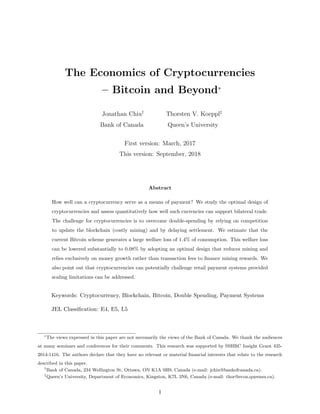
30. Figure 5.1: Size Distribution of Bitcoin Transactions (Ron and Shamir, 2013)
10 Dorit Ron, Adi Shamir
scheme actually enables sending micro transactions, which are of the order of
10−8
BTC (this is the smallest fraction into which a BTC can be broken, and
is called a satoshi). When we also consider midsize amounts, we see that 73%
(84%) of the transactions involve fewer than 10 BTC’s. On the other hand, large
transactions are rare at Bitcoin: there are only 364 (340) transactions larger
than 50,000 BTC’s. We have carefully inspected all these large transactions and
describe our findings in the next section.
Larger or equal to Smaller than Number of transactions Number of transactions
in the graph of entities in the graph of addresses
0 0.001 381,846 2,315,582
0.001 0.1 1,647,087 4,127,192
0.1 1 1,553,766 2,930,867
1 10 1,628,485 2,230,077
10 50 1,071,199 1,219,401
50 100 490,392 574,003
100 500 283,152 262,251
500 5,000 70,427 67,338
5,000 20,000 6,309 6,000
20,000 50,000 1,809 1,796
50,000 364 340
It is interesting to investigate the most active entities in the Bitcoin system,
those who have either maximal incoming BTC’s or maximal number of trans-
actions. 19 such entities are shown in Table 7 sorted in descending order of the
number of accumulated incoming BTC’s shown in the third column. The left-
most column associates the entities with letters between A to S out of which
three are identified: B is Mt.Gox, G is Instawallet and L is Deepbit. Eight ad-
ditional entities: F, H, J, M, N, O, P, and Q are pointed out in the graph of
the largest transactions (Fig. 1) which is presented in the next section. The sec-
ond column gives the number of addresses merged into each entity. The fourth
column presents the number of transactions the entity is involved with.
Table 7 shows that Mt.Gox has the maximal number of addresses, but not
the largest accumulated incoming BTC’s nor the largest number of transactions.
Entity A in the first row of Table 7 owns the next largest number of addresses,
about 50% of those of Mt.Gox’s, but received 31% more BTC’s than Mt.Gox.
Deepbit had sent 70% more transactions than Mt.Gox. It is interesting to re-
alize that the number of addresses of 13 of these entities is a fifth or more of
the number of transactions they have executed, which may indicate that each
address is indeed used for just a few transactions. It is also clear that six out
of the 19 entities in the table have each sent fewer than 30 transactions with a
total volume of more than 400,000 BTC’s. Since these entities were using large
transactions, we were able to isolate them and to follow the flow of their trans-
−15 −10 −5 0 5 10
0
0.05
0.1
0.15
0.2
0.25
0.3
0.35
log(ε)
f(ε)
10
−15
10
−10
10
−5
10
0
10
5
10
10
0
10
20
30
40
50
60
70
x
N(x)
Figure 5.2: Density of Preference Shocks F(ε) and Confirmation Lag N(x)
30

31. 0 0.02 0.04
2.57
2.575
2.58
2.585
x 10
5
σ
B
E(x)
0 0.02 0.04
0
10
20
30
40
50
Wgt.
Avg.
N
0 0.02 0.04
9.8845
9.8846
9.8846
9.8847
9.8847
9.8848
9.8848
x 10
6
Utility
0 0.02 0.04
9.8834
9.8836
9.8838
9.884
9.8842
9.8844
9.8846
x 10
6
Welfare
0 0.02 0.04
0
2
4
6
8
10
R
0 0.02 0.04
0
500
1000
1500
Mining
Cost
Figure 5.3: Effects of money growth
5.3 Efficiency of Cryptocurrencies
For the distribution of preference shocks in Figure 5.1, Table 5.3 evaluates the efficiency of Bitcoin
as a means of payment relative to a cash system. All computations are for our benchmark model
with the same preference parameters, but using different payments systems: cash, Bitcoin, optimal
reward structure for Bitcoin. Besides mining costs, we report two measures of the welfare cost.
The first measure gives the fraction of consumption people are willing to sacrifice in order to use
cash under the Friedman rule which implies zero welfare costs. The second one computes the
inflation rate with traditional cash so that people are indifferent between such system and the
cryptocurrency.
The current Bitcoin design is very inefficient, generating a welfare loss of 1.4% relative to an efficient
cash system.27 The main source for this inefficiency is the large mining cost, which is estimated to
be 360 mn USD per year. This translates into people being willing to accept a cash system with
an inflation rate of 230% before being better off using Bitcoin as a means of payment.
27
For comparison, a cash system with a 2% money growth rate generates a relatively small welfare cost of 0.003%.
31

32. However, given the distribution of preference shocks, it is inefficient to set the money growth rate
and the transaction fees as high as in the calibrated model for Bitcoin. The optimal policy is
to reduce the money growth rate – and to not use transaction fees at all (see Proposition 8) –
which will discourage mining substantially. Consequently, an optimally designed reward structure
for Bitcoin would reduce its welfare cost to a small fraction of its estimated current cost (0.08%).
The corresponding inflation that leaves people indifferent would drop to a more moderate level of
27.51%.
Still, relative to cash, Bitcoin seems to be a very inefficient payment system for facilitating the
observed set of transactions. This result could be driven by the fact that in the data, Bitcoin is
being used for both large and small value transactions, and that the total volume of transactions
is small. In order to control for this, we examine next the efficiency of a cryptocurrency when it is
used to support a large volume of either small or large value transactions.
Table 5.3: Efficiency of Current and Optimal Cryptocurrency Systems
Bitcoin (benchmark) Bitcoin (optimal policy)
µ − 1 9.5% 0.17%
τ 0.0088% 0%
welfare loss 1.41% 0.08%
mining cost (per year) $359.98 millions $6.90 millions
equivalent inflation tax 230.44% 27.51%
5.4 Best Usage of Cryptocurrencies
We now evaluate the efficiency of using cryptocurrencies for retail and large-value settlement sys-
tems. In Table 5.4, we present the quantiative results of calibrating our cryptocurrency model to
2014 US retail (debit cards) payments data and US large-value (Fedwire) data. A period is 30
minutes and the block length 1 minute. For the retail data, we pick B = 30.16 millions to match
the number of debit cards28 and set σ = 0.540853348 to match the volume of transactions per card
per day. For Fedwire, we assume B = 7866 to match the number of participants in 2014, and set
σ = 0.9795 which is the average volume of transactions for a participants in 30 minutes. Finally, we
28
Source: http://www.bis.org/cpmi/publ/d152.pdf
32

33. Table 5.4: Welfare Comparison between Retail and Large-value Systems
Retail Payments Large Value Payments
(US Debit cards) (Fedwire)
avg transaction size $38.29 $6,552,236
annual volume 59539 millions 135 millions
optimal µ − 1 0.038% 0.53%
optimal τ 0% 0%
confirmation lag 2 mins 12 mins
welfare loss 0.00052 % 0.0060%
mining cost (per year) $4.33 millions $22.10 billions
equivalent fee (per transfer) $0.0002 $392.56
chose ε so that the average size of transactions equals the one observed in these payments systems,
$38.29 and $6.5mn respectively. This is driven by data limitations. Double-spending incentives
however increase with transaction size and, hence, we assume that the largest transactions in the
debit card and Fedwire systems are 100 times and 5 times the average trade size.
Table 5.4 confirms that the welfare losses in a retail payment system are much smaller than in a
large-value one. In terms of the consumption equivalent measure, the welfare loss in a larger-value
system is 0.006% of consumption, which is about 10 times larger than that in a retail system. A
large-value system incurs a huge mining cost of 22 bn USD, which is over 5000 times of that in
the retail system. In the last row, we also derive the required transaction fee of a cash system (at
2% inflation) so that people are indifferent between such system and the cryptocurrency. When
a cryptocurrency is used for retail transactions, the equivalent transaction fee is a negligible 0.02
cents per transfer. For the large-value system, the corresponding fee becomes a very large $392.
The basic intuition follows directly from the double spending constraint we have derived in our
theoretical model. As the transaction size is smaller in the retail system, the incentives to double
spend are also smaller. Furthermore, mining is a public good so that the rewards from money
growth can support a large transaction volume. This implies that confirmation lags can be shorter
and one needs to induce less mining effort to dwarf double spending. Consequently, money growth
can also be smaller in a retail system, making a cryptocurrency system less costly due to inflation.
33

34. This implies that a cryptocurrency works best when the volume of transactions is larger relative to
the individual transaction size. As a result, a cryptocurrency tends to be much more efficient for
conducting retail payments.
The transaction fee measures in the last row of the table allow us to also evaluate whether cryp-
tocurrencies can be a viable alternative to currenct payment systems. The interchange fee in the
current debit card system is about 23 cents per transfer, while the service fee for Fedwire is 82 cents
per transfer.29 This suggests that a well-functioning cryptocurrency system can potentially chal-
lenge current debit card systems by offering users a competitive transaction fee with large enough
transaction volumes.
This comparison – especially for retail payments systems – needs to be interpreted with caution.
First, we do not consider certain private costs of running a cryptocurrency system. Examples
are costs for data storage, network communication and software such as wallets to operate the
system. Second, while the mining cost is a deadweight loss to society, part of the fees collected by
retail and large value payment systems are profits earned by the providers so that operating costs
tend to be lower than reflected in those fees. Finally, the above comparison does not take into
account an important technical limitation of cryptocurrencies. Bitcoin and other implementations
of cryptocurrencies face tight limits to their scalability. Unless one can address this issue by
changing limits on block size and latency due to network speed, such systems will not be able to
handle a large volume of transactions as required by modern retail payment systems.
6 Conclusion
Distributed record-keeping with a blockchain based on consensus through PoW is an intriguing
concept. The economics of this technology that underlies most cryptocurrencies are driven by the
individual incentives to double-spend and the costs associated with reining in these incentives.
These costs are private in the form of settlement delay and social in the form of mining which is
a public good. Consequently, as the scale of a cryptocurrency increases, it becomes more efficient.
This explains why a double-spending proof equilibrium exists only when the user pool is sufficiently
large, and why a cryptocurrency works best when the volume of transactions is large relative to
29
For the detail, see https://www.federalreserve.gov/paymentsystems/regii-average-interchange-fee.htm and
https://www.frbservices.org/servicefees/fedwire funds services 2017.html.
34

35. the individual transaction size. This insight seems to be very much ignored in the current debate,
but puts scalability of cryptocurrencies front and centre as the main technological challenge to be
overcome. Our exercise shows that cryptocurrency systems can potentially be a viable alternative
to retail payment systems, as soon as some technological limits can be resolved.30
For Bitcoin we find that it is not only extremely expensive in terms of its mining costs, but also
inefficient in its long-run design. However, the efficiency of the Bitcoin system can be significantly
improved by optimizing the rate of coin creation and minimizing transaction fees. Another poten-
tial improvement is to eliminate inefficient mining activities by changing the consensus protocol
altogether. In the Appendix, we explore the possibility of replacing PoW by a Proof-of-Stake (PoS)
protocol. Our analysis finds conditions under which PoS can strictly dominate PoW and even sup-
port immediate and final settlement. Notwithstanding, as we point out in this Appendix as well,
many fundamental issues of a PoS protocol remain still to be sorted out. There remains much to be
learned about the economic potential and the efficient, economic design of blockchain technology.
References
Agarwal, R. and M. Kimball, (2015). “Breaking through the Zero Lower Bound.”Working Paper
WP/15/224, International Monetary Fund.
Aumann, Robert J. (1965). “Integrals of set-valued functions”, Journal of Mathematical Analysis
and Applications, 12.1, 1-12.
Berentsen, A. (197). “Monetary policy implications of digital money”, Kyklos, 51(1), 89-117.
Biais, B., Bisière, C., Bouvard, M. and Cassamatta, C. (2017), “The Blockchain Folk Theorem”,
Working paper 817, Toulouse School of Economics.
30
As pointed out by Christine Lagarde, the head of the International Monetary Fund, cryptocurrencies could in
time be embraced more broadly: “For now, virtual currencies such as Bitcoin pose little or no challenge to the
existing order of fiat currencies and central banks ... But many of these [impediments] are technological challenges
that could be addressed over time. Not so long ago, some experts argued that personal computers would never
be adopted, and that tablets would only be used as expensive coffee trays. So I think it may not be wise to
dismiss virtual currencies.” Source: https://www.imf.org/en/News/Articles/2017/09/28/sp092917-central-banking-
and-fintech-a-brave-new-world
35

36. Böhme, R., Christin, N., Edelmann, B. and Moore, T. (2015), “Bitcoin: Economics, Technology
and Governance”, Journal of Economic Perspectives, vol. 29, pp. 213-238.
Bordo, M. and Levin, A. (2017), “Central Bank Digital Currency and the Future of Monetary
Policy”, Economics Working Paper 17104, Hoover Institution.
Camera, G. (2017). “A Perspective on Electronic Alternatives to Traditional Currencies”, Sveriges
Riksbank Economic Review, 2017:1, 126-148.
Chiu, J., and T. Wong. (2015). “On the Essentiality of E-Money”, Working Paper 2015-43, Bank
of Canada.
Fernández-Villaverde, J. and D. Sanches, (2016). “Can currency competition work?”, NBER Work-
ing Paper 22157, National Bureau of Economic Research.
Gandal, N., and H. Halaburda (2014). “Competition in the Cryptocurrency Market”, Working
Paper 2014-33, Bank of Canada.
Gans, J., and H. Halaburda, (2013). “Some Economics of Private Digital Currency”, Working Paper
2013-38, Bank of Canada.
Glaser, F., Haferkorn, M., Weber, M. amd Zimmermann, K. (2014), “How to price a Digital
Currency? Empirical Insights in the Influence of Media Coverage on the Bitcoin Bubble”, Banking
and Information Technology, 15.
Huberman, G., Leshno, J. and Moallemi, C. (2017), “Monopoly without a Monopolist: An Eco-
nomic Analysis of the Bitcoin Payment System”, Working Paper 17-92, Columbia Business
School.
Koeppl, T., Monnet, C. and Temzelides, T. (2008), “A Dynamic Model of Settlement”, Journal of
Economic Theory, 142, pp. 233-246.
Koeppl, T., Monnet, C. and Temzelides, T. (2012), “Optimal Clearing Arrangements for Financial
Trades”, Journal of Financial Economics, 103, pp. 189-203.
Lagos, L. and Wright, R. (2005). “A unified framework for monetary theory and policy analysis ”,
Journal of Political Economy, 113, pp. 463-484.
36

37. Moore, T. and N. Christin, (2013). “Beware the Middleman: Empirical Analysis of Bitcoin-
Exchange Risk”, in: Financial Cryptography and Data Security, Springer.
Rogoff, K.S., (2016). The Curse of Cash, Princeton University Press.
Ron, D. and Shamir, A. (2013). “Quantitative analysis of the full bitcoin transaction graph”,
International Conference on Financial Cryptography and Data Security, pp. 6-24.
Rosenfeld, M. (2014) “Analysis of hashrate-based double spending”, arXiv preprint,
arXiv:1402.2009.
Yermack, D. (2013) “Is Bitcoin a real currency? An economic appraisal”, No. w19747. National
Bureau of Economic Research.
37

38. A Appendix – Proofs and Derivations
A.1 A micro-foundation for the proof-of-work problem
Miners perform their mining between trading sessions. By investing computing power q(m), the
probability that a miner m can solve the computational task within a time interval t is given by
an exponential distribution with parameter µm
F(t) = 1 − e−µmt
where µm = q(m)/D. The parameter D captures the difficulty of the proof-of-work controlled by
the system. The expected time needed to solve the problem is thus given by
D
q(m)
.
Aggregating over all M miners, the first solution among all miners, min(τ1, τ2..., τM ), is also an ex-
ponential random variable with parameter
PM
m=1 µm. Hence the expected time needed to complete
the proof-of-work by the pool of miners is31
D
PM
m=1 q(m)
.
Furthermore, any particular miner m will be the first one to solve the proof-of-work problem with
probability
ρn =
q(n)
PM
m=1 q(m)
.
31
In practice, the parameter D is often adjusted to maintain a constant time for completing the proof-of-work
problem given any changes in the total computational power.
38

39. A.2 Proof of Lemma 2
Proof. This is true for s = 0. Suppose the result holds true for s = n − 1. Consider s = n,
qN−n(d, N) =
p
QM · DN−n+1(d, N) − QM (A.1)
= βR(
√
∆ − n) − βR (A.2)
= βR[
√
∆ − (n + 1)]. (A.3)
ρN−n(d, N) =
qN−n(d, N)
QM + qN−n(d, N)
(A.4)
=
√
∆ − (n + 1)
√
∆ − n
. (A.5)
DN−n(d, N) = ρN−n(d, N)DN−n+1(d, N) − qN−n(d, N) (A.6)
=
√
∆ − (n + 1)
√
∆ − n
βR(
√
∆ − n)2
− βR[
√
∆ − (n + 1)] (A.7)
= βR[(
√
∆ − (n + 1)]2
. (A.8)
39

40. A.3 Suboptimal to quit mining after winning a block
Claim: If a DS plan (q0, ..., qN ) generates a positive payoff, then the buyer has no incentives to quit
mining after winning a block in n N.
Proof : Consider the case with N = 2
D0 = ρ0ρ1ρ2
β
µ
[d + 3R] − ρ0ρ1q2 − ρ0q1 − q0
= ρ0





ρ1
ρ2
β
µ
[d + 3R] − q2
| {z }
D2
−q1





| {z }
D1
−q0
Define D1 = ρ1
h
ρ2
β
µ [d + R(1 + N)] − q2
i
− q1. Since
D0 = ρ0D1 − q0 0
we must have
ρ1
ρ2
β
µ
[d + 3R] − q2
− q1
β
µ
R. (A.9)
Similarly, define D2 = ρ2
β
µ [d + R(1 + N)] − q2. Condition (A.9) becomes
ρ1D2 − q1
β
µ
R,
which implies that D2 2β
µ R, or
ρ2
β
µ
[d + R(1 + N)] − q2 2
β
µ
R. (A.10)
Condition (A.10) implies that
ρ2
β
µ
[d + 3R] − q2 + u(x) 2
β
µ
R +
β
µ
d.
Here, the LHS is the expected payoff of continuing DS in session 2, and the RHS is the payoff of
quitting DS.
Similarly, condition (A.9) implies that
ρ1
ρ2
β
µ
[d + 3R] − q2
− q1 + δu(x)
β
µ
R +
β
µ
d.
40

41. Here,the LHS is the expected payoff of continuing DS in session 1, and the RHS is the payoff of
quitting DS.
For a general N, we can show that
DN = ρN
β
µ
[d + R(1 + N)] − qN
β
µ
NR,
DN−1 = ρN−1DN − qN−1
β
µ
(N − 1)R,
.
.
.
D1 = ρ1D2 − q1
β
µ
R,
D0 = ρ0D1 − q0 0.
They imply respectively
ρN
β
µ
[d + R(1 + N)] − qN + u(x)
β
µ
(NR + d),
ρN−1DN − qN−1 + δu(x)
β
µ
[(N − 1)R + d],
.
.
.
ρ1D2 − q1 + δN−1
u(x)
β
µ
(R + d).
Hence, there is no incentives to quit after winning a block.
41

42. A.4 A condition for no double spending
We now derive a sufficient condition under which double-spending contracts are dominated in
equilibrium. Define the nominal interest rate as i = µ/β − 1.
Lemma A.1. Only DS-proof contracts are offered if
δεmaxu0
(x̄1)(1 − τ)
3
4
− 1
i
σ
(A.11)
where x̄1 = (1 − τ)(β/µ)2R and i = µ/β − 1.
Proof: We examine the optimal DS contract and the optimal DS-proof contract.
DS-proof contract
Fix N. The optimal DS-proof contract is a solution to
max
d,x
−d + (1 − σ)
β
µ
d + σδN
εu(x)
subject to
x
1 − τ
µ
β
= d
d ≤ R(N + 1)N
Note that the participation constraint of the seller is always binding.
If the incentive constraint is not binding, then the FOC is then given by
1 =
σ
i
[δN
εu0
(x)(1 − τ) − 1],
where i = µ/β − 1 is the nominal interest rate. We denote this solution by (x∗, d∗) where it is
understood that the solution depends on N.
If the incentive constraint is binding, then we have that
¯
d = R(N + 1)N
x̄(N) =
β
µ
(1 − τ)R(N + 1)N
and
1
σ
i
[δN
εu0
(x̄(N))(1 − τ) − 1]
42

43. We denote this solution by (x̄, ¯
d) where it is understood that the solution depends on N.
DS contract
Fix N. The optimal DS contract is a solution of the problem
max
d,x
−d + (1 − σ)
β
µ
d + σ δN
εu(x) + D0(d, N)
subject to
x
1 − τ
µ
β
= d(1 − P(d, N))
1 − P(d, N) =
(N + 1)
√
∆
d ≥ R(N + 1)N
Note that the participation constraint for the seller is binding again.
Some preliminaries first.
∂D0(d, N)
∂d
=
β
µ
P(d, N)
∂P(d, N)
∂d
=
1
2R∆
(1 − P(d, N))
∂d(1 − P(d, N))
∂d
=
1 −
d
2R∆
(1 − P(d, N))
We look next at the function d(1 − P(d, N)). First, note that this expression is only valid when
d ≥ ¯
d. Its minimum is achieved at ¯
d. It is strictly increasing in d and strictly concave.
Differentiating the objective function w.r.t. to d, we obtain up to a factor of β
µ
−i + σ(1 − P(d, N))
δN
εu0
(x)(1 − τ)
1 −
d
2R∆
− 1
Case 1:
Suppose now that for a given N we have x∗ x̄, that is at the best DS-proof contract the constraint
is not binding.
Since (1 − P(d, N)) 1 and (1 − d/(2R∆)) 1, we have immediately that the objective function
is decreasing in d. Hence, the best DS contract has d = ¯
d. But this is worse than (x∗, d∗).
Case 2:
43

44. Suppose now that for a given N we have x̄ x∗ so that the constraint is binding for the optimal
DS-proof contract.
Note first that the objective function is strictly concave. This implies that there is a unique
maximizer and – by the previous argument – the solution needs to satisfy x̂ ∈ [x̄, x∗).
A sufficient condition is thus that the objective function is decreasing at x̄. The first-order condition
at x̄ is given by
−i + σ
δN
εu0
(x̄)(1 − τ)
1 −
1
2
N
N + 1
− 1
(A.12)
Finally, note that this equation is strictly decreasing in N as u0(x̄) is decreasing in N. Hence, a
sufficient condition is that the objective function is decreasing at N = 1 and ¯
d or, equivalently, that
δεu0
[(1 − τ)(β/µ)2R](1 − τ)
3
4
≤
i + σ
σ
.
So we can conclude that DS is never optimal when
δεmaxu0
(x̄(1))(1 − τ)
3
4
− 1
i
σ
where x̄(1) = (1 − τ)(β/µ)2R.
How to interpret condition (A.11)? Note that in general, the marginal value of an additional unit
of money balances is (proportional to)
−i + (1 − P)σ[δN
εu0
(x)(1 − τ)E(x) − 1]
where
E(x) =
∂x
∂d
d
x
=
∂
∂d
[d(1 − P(d, N))]
1
d[1 − P(d, N)]
=



1 , if x x̄
1 − d
2R∆ , if x ≥ x̄
is the elasticity of consumption with respect to money balances. When the incentive constraint is
not binding, E = 1. When it is binding, E 1. Define x̄N as the maximum DS-proof quantity
given N. Evaluating at x̄N ,
E(x̄N ) = 1 −
N
2(1 + N)
44

45. which is a decreasing function with its maximum equals to 3/4 when N = 1. The idea is that
when the incentive constraint is binding, a further increase of the trade size will raise the buyer’s
incentive to double spend after trade, hence lowering the effective value of a marginal dollar.
This condition tends to be satisfied when (i) the cost of bringing the extra money balances is high
(i is high), (ii) the probability of spending that extra balances is low (σ is low), and (iii) the utility
gain from spending that balances is low (δ, εmax are low or x̄ is high).
45

46. A.5 Proof of Proposition 7
We aim to show that a DS-proof cryptocurrency equilibrium exists for a sufficiently large B.
We will proceed in two steps. First, we show the existence under the assumption that only DS-
proofs contracts are offered. Second, we will show that condition (A.11) is satisfied so that the
derived equilibrium is DS-proof.
Step 1
Suppose condition (A.11) is satisfied. Define the correspondence
ϕ(R) = B
µ − 1 + στ
N̄ + 1
Z
z(ε, R)dF(ε)
where
R
z(ε, R)dF(ε) is aggregate money demand. The correspondence ϕ expresses total rewards
for mining as a function of aggregate money demand which itself is a function of R through the
double-spending constraint.
We need to show that the correspondence ϕ has a fixed point for some R. Given this R, the money
demand will determine the optimal offer (x(ε), d(ε), N(ε)) for all ε, where d(ε) = z(ε), so that we
have an equilibrium.
We will use Kakutani’s fixed point theorem. This implies that
(i) we need to restrict the mapping ϕ to be from a non-empty, convex and compact set
and
(ii) ϕ is non-empty, upper hemicontinuous, convex-valued and closed-valued.
To do so, it is useful to define zn(ε; R) which is the optimal money demand given R conditional on
choosing confirmation lag n ∈ {1, . . . , N̄}. The functions zn(ε; R) are continuous by the Theorem
of the Maximum and weakly increasing in R.
Lemma A.2. Fix Rmin arbitrarily close to 0. There exists a sufficiently large B(Rmin) such that
ϕ(R) ≥ Rmin for all R ≥ Rmin.
Proof. Choose Rmin small. For any R 0, we have that z∗(R; ε) 0 for any ε given our assumptions
on the utility function. Since zn(ε; R) is weakly increasing in R, we can find a B sufficiently large
46

47. for any Rmin close to 0 such that
B
µ − 1 + στ
N̄ + 1
Z
z(ε; R)dF(ε) ≥ B
µ − 1 + στ
N̄ + 1
Z
min
n
zn(ε; R)dF(ε) Rmin (A.13)
for all R ≥ Rmin.
Lemma A.3. Given B(Rmin), there exists Rmax such that ϕ(Rmax) ≤ Rmax.
Proof. The surplus from bringing z balances in the market is bounded by
βσ(εu(x∗
) − x∗
) − (1 − β/µ)z (A.14)
where x∗ satisfies εu0(x∗) = 1. Hence, there is an upper bound z̄(ε) on money demand that is
independent of R. Thus, for all R, we have that
ϕ(R) ≤ Rmax = B(Rmin)
µ − 1 + στ
N̄ + 1
Z
z̄(ε)dF(ε) (A.15)
These two lemmata allow us to restrict the correspondence ϕ to a compact interval [Rmin, Rmax]
where ϕ(R) : [Rmin, Rmax] → [Rmin, Rmax]. We turn next to the properties of the correspondence
ϕ.
Lemma A.4. The money demand correspondence z(R; ε) is non-empty, compact-valued and u.h.c.
Proof. Take the optimal money demand functions conditional on n and form the constraint corre-
spondence
Z =
N̄
[
n=1
zn(R; ε). (A.16)
Note that this correspondence is both u.h.c. and l.h.c, hence continuous. Furthermore, it is
compact-valued as it is comprised of a finite number of values.
Let Vn(R) be the value associated utility with zn(R; ε). Then, the optimal money demand is given
by
max
n
Vn(R) (A.17)
subject to
zn(R) ∈ Z (A.18)
47

48. By the Theorem of the Maximum, we have that the correspondence of the maximizer z(R; ε) is non-
empty and u.h.c. Since it comprises only a finite number of elements, it is also compact-valued.
It follows immediately that the correspondence ϕ(R) is also non-empty, compact-valued and convex-
valued (see Aumann (1965), Theorem 1,2 and 4). Furthermore, ϕ(R) is u.h.c (see Aumann (1965),
Corollary 5.2). By Kakutani’s Fixed Point theorem, there exists R∗ ∈ [Rmin, Rmax] such that
R∗
∈ ϕ(R∗
)
which completes the proof.
Step 2
To ensure that only DS-proof contracts are offered, notice that condition (A.11)
δεmaxu0
[
2β(1 − τ)
µ
R](1 − τ)
3
4
− 1
µ − β
σβ
defines a threshold R̄min such that the condition is satisfied for all R R̄min. By setting Rmin =
R̄min in step 1, we can ensure that the equilibrium determined by the fixed point is DS-proof.
48

49. A.6 Proof of Proposition 8
Proposition A.5. The optimal reward structure sets transaction fees to zero and only relies on
seignorage; i.e., τ = 0 and µ 1.
The idea of the proof is as follows. If fees are not zero, one can design a new policy that (i) relies
on less costs for mining and (ii) makes all buyers better off. The policy change will combine three
changes. First, it reduces transaction fees to zero. Second, it will increase the seignorage rate
to compensate for the loss in the expected tax rates from fees. Third, it will generate a revenue
for miners given these changes that does not change the choice set for any individual bilateral
transaction.
We then proceed as follows. First, we show that the policy change is feasible and that it improves
the planner’s objective provided that the transaction size and confirmation lags weakly increase in
all bilateral meetings. Then, we show that buyers have an incentive to only change their optimal
offer in that way.
The proof relies on the fact that the planner can generate more revenue than the amount of rewards
paid out to miners. This implies that the planner can have extra revenue available in the centralized
market after the policy change. We then show further that, if the extra revenue is positive, the
planner can make everyone (weakly) better off by reducing seignorage to lower revenue. This implies
that it is optimal to collect seignorage just enough to finance mining costs.
A.6.1 Preliminaries
The social planner’s problem is given by
max
µ,τ,R
B
Z
σ[δN(ε)
εu(x(ε)) − x(ε)]dFε(ε) −
β
µ
R(N̄ + 1) (A.19)
subject to
(d(ε), x(ε), N(ε)) is an optimal offer for any (µ, τ, R) (A.20)
B(µ − 1 + στ)
Z
x(ε)
1 − τ
dFε(ε) ≥
β
µ
R(N̄ + 1) (A.21)
Note that we have assumed that the sufficient condition for No-DS offers is satisfied. Hence, all
49

50. offers satisfy the no-DS constraint
µ
β
x(ε)
1 − τ
≤ R(N(ε) + 1)N(ε).
Note also that the revenue constraint (A.21) is a weak inequality. This implies that the planner is
allowed to achieve a (non-negative) surplus by choosing any particular policy. It is understood that
this surplus could be distributed in the centralized market to anyone – miner, sellers or buyers – as
a lump-sum transfer without affecting the total surplus as there is no wealth effect due to agents’
quasi-linear preferences. Importantly, the planner makes thus a distinction between the revenue
raised and the rewards paid to miners. Hence, we define a policy to be (µ, τ, R).
A.6.2 A welfare-improving policy change
Suppose that τ0 0, µ0 ≥ 1 and R0 is a feasible policy. Consider the following policy change
τ1 = τ0 − ξ (A.22)
µ1 = µ0 + σξ (A.23)
R1 = R0
1 − τ0
1 − τ1
µ1
µ0
(A.24)
Note that the rewards R1 that flow to miners are also adjusted in the policy change. Also note
that τ0 ≥ ξ 0 is arbitrary and, thus, we can set it to τ0.32
We denote the optimal choice for each policy by x∗
i (ε) and show first that this policy change is
feasible if the transaction size increases in all bilateral meetings.
Lemma A.6. The policy change is feasible if x∗
1(ε) ≥ x∗
0(ε).
Proof. The No-DS for the old policy is given by
µ1
β
x(ε)
1 − τ1
≤ R1(N(ε) + 1)N(ε) (A.25)
Using the definition of R1, it is immediate that – by construction – the constraints are identical for
all given n ∈ {1, . . . , N̄ − 1}, no matter what the value of ε ∈ (0, τ0] is. Hence, the set of feasible
choices for bilateral meetings remains unchanged.
32
COMMENT: It will become clear later that raising seignorage is not an issue. See Laffer curve.
50

51. Next, we show that the revenue constraint is also fulfilled as long as the optimal individual trans-
action sizes do not decreases. We have
B(µ1 − 1 + στ1)
Z
x1(ε)
1 − τ1
dFε(ε) (A.26)
≥ B(µ0 + σξ − 1 + στ0 − σξ)
Z
x0(ε)
1 − τ1
dFε(ε) (A.27)
≥
β
µ1
R0
1 − τ0
1 − τ1
µ1
µ0
(N̄ + 1) (A.28)
=
β
µ1
R1(N̄ + 1) (A.29)
which completes the proof.
Next, we show that the policy change increases the planner’s objective as long as consumption
and confirmation lags weakly increase for all individual bilateral meetings. We denote the optimal
confirmation lags for the two policies by N0 and N1 and the optimal transaction sizes by x0 and
x1, respectively.
Lemma A.7. Suppose that x1(ε) ≥ x0(ε) and N1(ε) ≥ N0(ε). The policy change then increases
the planner’s objective function.
Proof. First, consider the mining costs. We have
β
µ1
R1(N̄ + 1) =
β
µ0
R0
1 − τ0
1 − τ0 + ξ
(N̄ + 1)
β
µ0
R0(N̄ + 1) (A.30)
so that the mining costs decrease.
Second, we can rewrite the trade surplus in the decentralized market for each ε as
σ[δN1
εu(x1) − x1] =
= σδN1
εu(x1) −
x1
1 − τ1
µ1
β
+ (1 − σ)
x1
1 − τ1
(A.31)
− σx1 +
x1
1 − τ1
µ1
β
− (1 − σ)
x1
1 − τ1
(A.32)
where the second line corresponds to the buyer’s objective function.
51

52. Since the buyer’s choice is optimal, we obtain from the condition in the lemma that
σ[δN1
εu(x1) − x1] = (A.33)
≥ σδN0
εu(x0) −
x0
1 − τ1
µ1
β
+ (1 − σ)
x0
1 − τ1
− σx1 +
x1
1 − τ1
µ1
β
− (1 − σ)
x1
1 − τ1
(A.34)
= σ[δN0
εu(x0) − x0] +
1
1 − τ1
µ1
β
− 1 + στ1
(x1 − x0) (A.35)
≥ σ[δN0
εu(x0) − σx0] (A.36)
which completes the proof.
Define N∗ as the buyer’s optimal choice of confirmation lag, and x∗(n) as the buyer’s optimal
choice of x, given a fixed confirmation lag n. We are now left to show that the optimal choice of
the buyer is to weakly increase both, the optimal size of the transaction and the confirmation lag
in the bilateral market. We do so in two steps, showing first that, for any given n, the optimal
choice x∗(n) is strictly increasing and then showing that the buyer is never better off lowering the
confirmation lag N∗.
Lemma A.8. Given n, the optimal choice x∗(n) is weakly increasing in the policy change for all
ε.
Proof. Define x∗(n) as the optimal quantity chosen by the buyer for any given n, that is
x∗
(n) = arg max
x
−
x
1 − τ
µ
β
+ (1 − σ)
β
µ
x
1 − τ
µ
β
+ σδn
εu(x) (A.37)
subject to
x
1 − τ
µ
β
≤ R(n + 1)n. (A.38)
The first-order condition is given by
σδn
εu0
(x) ≥
1
1 − τ
µ
β
− (1 − σ)
(A.39)
with equality when the No-DS constraint (A.38) is non-binding.
52

53. We have that
µ0
β
− (1 − σ)
(1 − τ1) −
µ1
β
− (1 − σ)
(1 − τ0) (A.40)
=
µ0
β
− (1 − σ)
(1 − τ0 + ξ) −
µ0 + σξ
β
− (1 − σ)
(1 − τ0) (A.41)
=
µ0
β
ξ − (1 − σ)ξ − (1 − τ0)
σ
β
ξ (A.42)
=
ξ
β
(µ − β(1 − σ) − σ + στ0) (A.43)
µ0 − 1 0 (A.44)
which shows that the right-hand side of the FOC is decreasing in the policy change – or, equivalently,
that the costs of financing any transaction level x are decreasing in the policy change. Consequently,
for any given n, the optimal choice is x∗
1(n) ≥ x∗
0(n).
Lemma A.9. Buyers choose N1 ≥ N0 given the policy change.
Proof. We first show that for any optimal choice all No-DS constraints must be binding for n N∗
and that x∗(n) x∗(N∗) for all n N∗.
Suppose to the contrary that the No-DS constraint is not binding for some n N∗. Denoting the
optimal choice conditional on n by x∗(n), we then have that
σδN∗
εu0
(x∗
(N∗
)) ≥ σδn
εu0
(x∗
(n)) =
µ
β
− (1 − σ)
1
1 − τ
(A.45)
with strict inequality if the No-DS constraint is binding at N∗.
Since n N∗, it must be the case that
x∗
(n) x∗
(N∗
). (A.46)
But this implies that x∗(N∗) is feasible with a confirmation lag n. Hence, N∗ cannot be optimal,
since choosing (x∗(N∗), n) is feasible, has the same cost, but earlier consumption. A contradiction.
By a similar argument, it is then straightforward to show that x∗(n) x∗(N∗), since otherwise
x∗(N∗) would be feasible with n and yield a higher utility than confirmation lag N∗.
Consider now the policy change where we denote . For all n N0, the No-DS constraints are still
binding. Hence, the choice conditional on n N0 remains unchanged despite the cost of x∗(n)
53

54. decreasing. We have
σδN0
εu(x0) − σδn
εu(x(n)) (A.47)
≥ (x0 − x(n))
1
1 − τ0
µ0
β
− (1 − σ)
(A.48)
(x0 − x(n))
1
1 − τ1
µ1
β
− (1 − σ)
(A.49)
since x0 x(n) and the last term is decreasing with the policy change. This implies that the
original choice at N0 still yields higher utility than the optimal choice for n N0 after the policy
change. Hence, the optimal choice must satisfy N1 ≥ N0 which completes the proof.
A.6.3 A Binding Revenue Constraint is Optimal
Any candidate optimal policy satisfies τ = 0 and µ 1. Suppose now that the revenue constraint
is not binding. Consider now a policy change according to
µ1 = µ0 − ξ (A.50)
R1 = R0
µ1
µ0
(A.51)
It follows immediately that Lemma A.6 still holds as long as ξ is sufficiently small. The reason is
that – by assumption – the revenue constraint was slack at (µ0, R0). Similarly, Lemma A.7 goes
through except for that the mining costs remain constant with the change now. Finally, nothing in
the remainder of the proof is affected by τ = 0 since larger transaction sizes become cheaper with
lower inflation. This implies that the proposed policy change can increase the planner’s objective
function. Note that, since τ = 0 and x(ε) is bounded, the revenue constraint (A.21) will become
binding for µ sufficiently close to 1.
This completes the argument.
This implies that the assumption of lump-sum rebates of extra revenue by the planner does not
matter for the argument at all, since the planner can choose lower seignorage if necessary once
transaction fees are zero.
54

55. B Appendix [FOR ONLINE PUBLICATION ONLY] – A formal
description of the blockchain
Aggregate State
Let mD
t (i) ≥ 0 denote the cryptocurrency balance held by agent i in the period t day market.
We then use SD
t = {mD
t (i)} to denote the entire public record of the holdings of these balances,
called the (aggregate) state. Similarly, mN
t,n(i) ≥ 0 and SN
t,n denote the balances and the state at
the beginning of the nth trading session of the period t night market. The economy starts with a
given initial state SD
0 .
Payments
We use ∆D
t (i, j) and ∆N
t,n(i, j) to denote respectively day and night transfers of balances from agent
i to agent j and call these transfers payments. A day payment is feasible if
∆D
t (i, j) ≥ 0,
mD
t (i) ≥
X
j
∆D
t (i, j).
Similarly, a night payment is feasible if
∆N
t,n(i, j) ≥ 0,
mN
t,n(i) ≥
X
j
∆N
t,n(i, j).
An agent can pay positive amounts to others and the total payments are bounded by the balances
one has accumulated.33 An agent’s balances accumulate over time as a result of net payment
inflows. Therefore, given any payments, the state is updated in the two markets according to
mN
t,0(i) = mD
t (i) +
X
j
∆D
t (j, i) − ∆D
t (i, j) + Tt(i), (B.1)
mN
t,n(i) = mN
t,n−1(i) +
X
j
∆N
t,n−1(j, i) − ∆N
t,n−1(i, j), for n = 1, ..., N̄ (B.2)
mD
t+1(i) = mN
t,N̄ (i) +
X
j
∆N
t,N̄ (j, i) − ∆N
t,N̄ (i, j) (B.3)
33
Through cryptography, the authenticity of payments is protected by digital signatures corresponding to the
sending addresses. As a result, only the owner of the digital signature can transfer balances to another address. This
gives rise to the non-negativity and the cash-in-advance constraints.
55

56. where T(i) denotes the potential transfers of new balances to agent i in the day market by the
cryptocurrency system.
Blockchain
Due to public monitoring, feasible payments during the day automatically update the aggregate
state according to the rule (B.1). The new state at the start of the night market is thus given by
SN
t,0 = ΨN
0 (SD
t , BD
t ) (B.4)
where BD
t = {∆D
t (i, j)} is the entire set of day transfers and is called a block. The update function
ΨN
0 is defined according to (B.1).
Payments in the night market, however, enter the state through a process we call mining. When
agent i makes a payment to agent j in the night, he needs to send out an instruction for a feasible
payment ∆N
t,n(i, j) to a pool of miners who compete to update the state with a new block of
feasible payments in session n of the night market. The set of feasible payment instructions BN
t,n =
{∆N
t,n(i, j)} is the nth block of period t payments in the night market.
A sequence of blocks {BD
t , {BN
t,n}N̄
n=0}T
t=0 iteratively generates a sequence of states {SD
t , {SN
t,n}N̄
n=0}T+1
t=0
according to
SN
t,0 = ΨN
0 (SD
t , BD
t )
SN
t,n = ΨN
n (SN
t,n−1, BN
t,n−1), for n = 1, ..., N̄
SD
t+1 = ΨD
(SN
t,N̄ , BN
t,N̄ ),
where the update functions ΨN
n , ΨD are defined by (B.1)-(B.3). We call the sequence of blocks
BT = {BD
t , {BN
t,n}N̄
n=0}T
t=0 a blockchain. Determined by the process of mining, one specific blockchain
is used to construct the public state and can be observed by everyone in the economy at all times.
56

57. C Appendix [FOR ONLINE PUBLICATION ONLY] – Proof of
Stake
We assume that the right for updating of the blockchain is allocated randomly across people. The
probability that one can update the chain is proportional to the unused balances in the night
market.
This is identical to pledging balances that are not used in transactions in order to gain a right
to update the chain. For simplicity, we assume that people can pledge balances after they learn
whether they have a match or not.
Denote the balances chosen in the day market for transaction purposes as d and the additional
amount of balances chosen for having a stake in the voting procedure as z0.
Whenever, z0 0, we have that there is a strictly positive probability that there is a double spend,
since the buyer in a transaction will propose a block that undoes the payment whenever he is
allowed doing so.
Fix N. The problem is given by
max
d,z0
− (z0
+ d) + σ
δN
u(x) +
β
µ
z0
+
z0
(1 − σ)Z
N+1
d +
z0
(1 − σ)Z
R(N̄ + 1)
!#
+
(1 − σ)
β
µ
z0
+ d +
z0 + d
(1 − σ)Z
R(N̄ + 1)
When having a transaction, a buyer is only allowed to update the chain if z0 0. Given N, he
needs to win the right to update N + 1 in order to double spend. If a buyer has no transaction, he
will pledge all his balances as a stake. Note that participation of the seller requires
x =
β
µ
d(1 − τ) 1 −
E(z0)
Z
N+1
!
.
Notice that the buyer’s choice of z0 is not observed by the seller, so x depends on seller’s expectation
E(z0) instead.
Lemma C.1. The objective function is strictly convex in z0 for all N ≥ 1 and linear in z0 for
N = 0.
Proof. Differentiating the objective function, we obtain
−i +
1
1 − σ
(στ + (µ − 1)) +
σ
1 − σ
(N + 1)
z0
(1 − σ)Z
N
d
Z
(C.1)
57