SlideShare uma empresa Scribd logo
1 de 62
Baixar para ler offline
1

Solution of Equations and
Eigen Value Problems
1.1 SOLUTION OF ALGEBRAIC AND TRANSCENDENTAL EQUATIONS
1.1.1 Introduction
A problem of great importance in science and engineering is that of determining the roots/
zeros of an equation of the form
f(x) = 0, (1.1)
A polynomial equation of the form
f(x) = Pn(x) = a0xn + a1xn–1 + a2xn–2 + ... + an –1x + an = 0 (1.2)
is called analgebraic equation. An equation which contains polynomials, exponential functions,
logarithmic functions, trigonometric functions etc. is called a transcendental equation.
For example,
3x3 – 2x2 – x – 5 = 0, x4 – 3x2 + 1 = 0, x2 – 3x + 1 = 0,
are algebraic (polynomial) equations, and
xe2x – 1 = 0, cos x – xex = 0, tan x = x
are transcendental equations.
We assume that the function f(x) is continuous in the required
interval.
We define the following.
Root/zero A number α, for which f(α) ≡ 0 is called a root of the
equation f(x) = 0, or a zero of f(x). Geometrically, a root of an equa-
tion f(x) = 0 is the value of x at which the graph of the equation y =
f(x) intersects the x-axis (see Fig. 1.1).
f(x)
O  x
Fig. 1.1 ‘Root of f(x) = 0’
2 NUMERICAL METHODS
Simple root A number α is a simple root of f(x) = 0, if f(α) = 0 and f ′(α) ≠ 0. Then, we can
write f(x) as
f(x) = (x – α) g(x), g(α) ≠ 0. (1.3)
For example, since (x – 1) is a factor of f(x) = x3 + x – 2 = 0, we can write
f(x) = (x – 1)(x2 + x + 2) = (x – 1) g(x), g(1) ≠ 0.
Alternately, we find f(1) = 0, f ′(x) = 3x2 + 1, f ′(1) = 4 ≠ 0. Hence, x = 1 is a simple root of
f(x) = x3 + x – 2 = 0.
Multiple root A number α is a multiple root, of multiplicity m, of f(x) = 0, if
f(α) = 0, f ′(α) = 0, ..., f (m –1) (α) = 0, and f (m) (α) ≠ 0. (1.4)
Then, we can write f(x) as
f(x) = (x – α)m g(x), g(α) ≠ 0.
For example, consider the equation f(x) = x3 – 3x2 + 4 = 0. We find
f(2) = 8 – 12 + 4 = 0, f ′(x) = 3x2 – 6x, f ′(2) = 12 – 12 = 0,
f ″(x) = 6x – 6, f ″(2) = 6 ≠ 0.
Hence, x = 2 is a multiple root of multiplicity 2 (double root) of f(x) = x3 – 3x2 + 4 = 0.
We can write f(x) = (x – 2)2 (x + 1) = (x – 2)2 g(x), g(2) = 3 ≠ 0.
In this chapter, we shall be considering the case of simple roots only.
Remark 1 A polynomial equation of degree n has exactly n roots, real or complex, simple or
multiple, where as a transcendental equation may have one root, infinite number of roots or
no root.
We shall derive methods for finding only the real roots.
The methods for finding the roots are classified as (i) direct methods, and (ii) iterative
methods.
Direct methods These methods give the exact values of all the roots in a finite number of
steps (disregarding the round-off errors). Therefore, for any direct method, we can give the
total number of operations (additions, subtractions, divisions and multiplications). This number
is called the operational count of the method.
For example, the roots of the quadratic equation ax2 + bx + c = 0, a ≠ 0, can be obtained
using the method
x =
1
2
4
2
a
b b ac
− ± −
L
N
M O
Q
P.
For this method, we can give the count of the total number of operations.
There are direct methods for finding all the roots of cubic and fourth degree polynomi-
als. However, these methods are difficult to use.
Direct methods for finding the roots of polynomial equations of degree greater than 4 or
transcendental equations are not available in literature.
SOLUTION OF EQUATIONS AND EIGEN VALUE PROBLEMS 3
Iterative methods These methods are based on the idea of successive approximations. We
start with one or two initial approximations to the root and obtain a sequence of approxima-
tions x0, x1, ..., xk, ..., which in the limit as k → ∞, converge to the exact root α. An iterative
method for finding a root of the equation f(x) = 0 can be obtained as
xk + 1 = φ(xk), k = 0, 1, 2, ..... (1.5)
This method uses one initial approximation to the root .
0
x The sequence of approxima-
tions is given by
x1 = φ(x0), x2 = φ(x1), x3 = φ(x2), .....
The function φ is called an iteration function and x0 is called an initial approximation.
If a method uses two initial approximations x0, x1, to the root, then we can write the
method as
xk + 1 = φ(xk – 1, xk), k = 1, 2, ..... (1.6)
Convergence of iterative methods The sequence of iterates, {xk}, is said to converge to the
exact root α, if
lim
k → ∞
xk = α, or lim
k → ∞
| xk – α | = 0. (1.7)
The error of approximation at the kth iterate is defined as εk = xk – α. Then, we can
write (1.7) as
lim
k → ∞
| error of approximation | = lim
k → ∞
| xk – α | = lim
k → ∞
| εk | = 0.
Remark 2 Given one or two initial approximations to the root, we require a suitable iteration
function φ for a given function f(x), such that the sequence of iterates, {xk}, converge to the
exact root α. Further, we also require a suitable criterion to terminate the iteration.
Criterion to terminate iteration procedure Since, we cannot perform infinite number of
iterations, we need a criterion to stop the iterations. We use one or both of the following
criterion:
(i) The equation f(x) = 0 is satisfied to a given accuracy or f(xk) is bounded by an error
tolerance ε.
| f (xk) | ≤ ε. (1.8)
(ii) The magnitude of the difference between two successive iterates is smaller than a given
accuracy or an error bound ε.
| xk + 1 – xk | ≤ ε. (1.9)
Generally, we use the second criterion. In some very special problems, we require to use
both the criteria.
For example, if we require two decimal place accuracy, then we iterate until | xk+1 – xk |
 0.005. If we require three decimal place accuracy, then we iterate until | xk+1 – xk |  0.0005.
As we have seen earlier, we require a suitable iteration function and suitable initial
approximation(s) to start the iteration procedure. In the next section, we give a method to find
initial approximation(s).
4 NUMERICAL METHODS
1.1.2 Initial Approximation for an Iterative Procedure
For polynomial equations, Descartes’ rule of signs gives the bound for the number of positive
and negative real roots.
(i) We count the number of changes of signs in the coefficients of Pn(x) for the equation f(x) =
Pn(x) = 0. The number of positive roots cannot exceed the number of changes of signs. For
example, if there are four changes in signs, then the equation may have four positive roots or
two positive roots or no positive root. If there are three changes in signs, then the equation
may have three positive roots or definitely one positive root. (For polynomial equations with
real coefficients, complex roots occur in conjugate pairs.)
(ii) We write the equation f(– x) = Pn(– x) = 0, and count the number of changes of signs in the
coefficients of Pn(– x). The number of negative roots cannot exceed the number of changes of
signs. Again, if there are four changes in signs, then the equation may have four negative
roots or two negative roots or no negative root. If there are three changes in signs, then the
equation may have three negative roots or definitely one negative root.
We use the following theorem of calculus to determine an initial approximation. It is
also called the intermediate value theorem.
Theorem 1.1 If f(x) is continuous on some interval [a, b] and f(a)f(b)  0, then the equation
f(x) = 0 has at least one real root or an odd number of real roots in the interval (a, b).
This result is very simple to use. We set up a table of values of f (x) for various values
of x. Studying the changes in signs in the values of f (x), we determine the intervals in which
the roots lie. For example, if f (1) and f (2) are of opposite signs, then there is a root in the
interval (1, 2).
Let us illustrate through the following examples.
Example 1.1 Determine the maximum number of positive and negative roots and intervals of
length one unit in which the real roots lie for the following equations.
(i) 8x3 – 12x2 – 2x + 3 = 0 (ii) 3x3 – 2x2 – x – 5 = 0.
Solution
(i) Let f(x) = 8x3 – 12x2 – 2x + 3 = 0.
The number of changes in the signs of the coefficients (8, – 12, – 2, 3) is 2. Therefore, the
equation has 2 or no positive roots. Now, f(– x) = – 8x3 – 12x2 + 2x + 3. The number of changes
in signs in the coefficients (– 8, – 12, 2, 3) is 1. Therefore, the equation has one negative root.
We have the following table of values for f(x), (Table 1.1).
Table 1.1. Values of f (x), Example 1.1(i).
x – 2 – 1 0 1 2 3
f(x) – 105 – 15 3 – 3 15 105
Since
f(– 1) f(0)  0, there is a root in the interval (– 1, 0),
f(0) f(1)  0, there is a root in the interval (0, 1),
f(1) f(2)  0, there is a root in the interval (1, 2).
SOLUTION OF EQUATIONS AND EIGEN VALUE PROBLEMS 5
Therefore, there are three real roots and the roots lie in the intervals (– 1, 0), (0, 1), (1, 2).
(ii) Let f(x) = 3x2 – 2x2 – x – 5 = 0.
The number of changes in the signs of the coefficients (3, – 2, – 1, – 5) is 1. Therefore,
the equation has one positive root. Now, f(– x) = – 3x2 – 2x2 + x – 5. The number of changes in
signs in the coefficients (– 3, – 2, 1, – 5) is 2. Therefore, the equation has two negative or no
negative roots.
We have the table of values for f (x), (Table 1.2).
Table 1.2. Values of f (x ), Example 1.1(ii).
x – 3 – 2 – 1 0 1 2 3
f(x) – 101 – 35 – 9 – 5 – 5 9 55
From the table, we find that there is one real positive root in the interval (1, 2). The
equation has no negative real root.
Example 1.2 Determine an interval of length one unit in which the negative real root, which is
smallest in magnitude lies for the equation 9x3 + 18x2 – 37x – 70 = 0.
Solution Let f(x) = 9x3 + 18x2 – 37x – 70 = 0. Since, the smallest negative real root in magni-
tude is required, we form a table of values for x  0, (Table 1.3).
Table 1.3. Values of f (x ), Example 1.2.
x – 5 – 4 – 3 – 2 – 1 0
f(x) – 560 – 210 – 40 4 – 24 – 70
Since, f(– 2)f(– 1)  0, the negative root of smallest magnitude lies in the interval
(– 2, –1).
Example 1.3 Locate the smallest positive root of the equations
(i) xex = cos x. (ii) tan x = 2x.
Solution
(i) Let f(x) = xex – cos x = 0. We have f(0) = – 1, f(1) = e – cos 1 = 2.718 – 0.540 = 2.178. Since,
f(0) f(1)  0, there is a root in the interval (0, 1).
(ii) Let f(x) = tan x – 2x = 0. We have the following function values.
f(0) = 0, f(0.1) = – 0.0997, f(0.5) = – 0.4537,
f(1) = – 0.4426, f(1, 1) = – 0.2352, f(1.2) = 0.1722.
Since, f(1.1) f(1.2)  0, the root lies in the interval (1.1, 1.2).
Now, we present some iterative methods for finding a root of the given algebraic or
transcendental equation.
We know from calculus, that in the neighborhood of a point on a curve, the curve can be
approximated by a straight line. For deriving numerical methods to find a root of an equation
6 NUMERICAL METHODS
f(x) = 0, we approximate the curve in a sufficiently small interval which contains the root, by
a straight line. That is, in the neighborhood of a root, we approximate
f(x) ≈ ax + b, a ≠ 0
where a and b are arbitrary parameters to be determined by prescribing two appropriate
conditions on f(x) and/or its derivatives. Setting ax + b = 0, we get the next approximation to
the root as x = – b/a. Different ways of approximating the curve by a straight line give different
methods. These methods are also called chord methods. Method of false position (also called
regula-falsi method) and Newton-Raphson method fall in this category of chord methods.
1.1.3 Method of False Position
The method is also called linear interpolation method or chord method or regula-falsi method.
At the start of all iterations of the method, we require the interval in which the root
lies. Let the root of the equation f(x) = 0, lie in the interval (xk–1, xk), that is, fk–1 fk  0, where
f(xk–1) = fk–1, and f(xk) = fk. Then, P(xk–1, fk–1), Q(xk, fk) are points on the curve f(x) = 0. Draw a
straight line joining the points P and Q (Figs. 1.2a, b). The line PQ is taken as an approxima-
tion of the curve in the interval [xk–1, xk]. The equation of the line PQ is given by
y f
f f
x x
x x
k
k k
k
k k
−
−
=
−
−
− −
1 1
.
The point of intersection of this line PQ with the x-axis is taken as the next approxima-
tion to the root. Setting y = 0, and solving for x, we get
x = xk –
x x
f f
k k
k k
−
−
−
−
F
HG I
KJ
1
1
fk = xk –
x x
f f
k k
k k
−
−
F
HG I
KJ
−
−
1
1
fk.
The next approximation to the root is taken as
xk+1 = xk –
x x
f f
k k
k k
−
−
F
HG I
KJ
−
−
1
1
fk. (1.10)
Simplifying, we can also write the approximation as
xk+1 =
x f f x x f
f f
k k k k k k
k k
( ) ( )
− − −
−
− −
−
1 1
1
=
x f x f
f f
k k k k
k k
− −
−
−
−
1 1
1
, k = 1, 2, ... (1.11)
Therefore, starting with the initial interval (x0, x1), in which the root lies, we compute
x2 =
x f x f
f f
0 1 1 0
1 0
−
−
.
Now, if f(x0) f(x2)  0, then the root lies in the interval (x0, x2). Otherwise, the root lies in
the interval (x2, x1). The iteration is continued using the interval in which the root lies, until
the required accuracy criterion given in Eq.(1.8) or Eq.(1.9) is satisfied.
Alternate derivation of the method
Let the root of the equation f(x) = 0, lie in the interval (xk–1, xk). Then, P(xk–1, fk–1), Q(xk, fk)
are points on the curve f(x) = 0. Draw the chord joining the points P and Q (Figs. 1.2a, b). We
SOLUTION OF EQUATIONS AND EIGEN VALUE PROBLEMS 7
approximate the curve in this interval by the chord, that is, f(x) ≈ ax + b. The next approximation
to the root is given by x = – b/a. Since the chord passes through the points P and Q, we get
fk–1 = axk–1 + b, and fk = axk + b.
Subtracting the two equations, we get
fk – fk–1 = a(xk – xk – 1), or a =
f f
x x
k k
k k
−
−
−
−
1
1
.
The second equation gives b = fk – axk.
Hence, the next approximation is given by
xk+1 = –
b
a
f ax
a
k k
= −
−
= xk –
f
a
k
= xk –
x x
f f
k k
k k
−
−
F
HG I
KJ
−
−
1
1
fk
which is same as the method given in Eq.(1.10).
y
O x
P x3
x2 x1
x0
Q
y
O x
P
x3
x2
x1
x0
Q
Fig. 1.2a ‘Method of false position’ Fig. 1.2b ‘Method of false position’
Remark 3 At the start of each iteration, the required root lies in an interval, whose length is
decreasing. Hence, the method always converges.
Remark 4 The method of false position has a disadvantage. If the root lies initially in the
interval (x0, x1), then one of the end points is fixed for all iterations. For example, in Fig.1.2a,
the left end point x0 is fixed and the right end point moves towards the required root. There-
fore, in actual computations, the method behaves like
xk+1 =
x f x f
f f
k k
k
0 0
0
−
−
, k = 1, 2, … (1.12)
In Fig.1.2b, the right end point x1 is fixed and the left end point moves towards the
required root. Therefore, in this case, in actual computations, the method behaves like
xk+1 =
x f x f
f f
k k
k
1 1
1
−
−
, k = 1, 2, … (1.13)
Remark 5 The computational cost of the method is one evaluation of the function f(x), for
each iteration.
Remark 6 We would like to know why the method is also called a linear interpolation method.
Graphically, a linear interpolation polynomial describes a straight line or a chord. The linear
interpolation polynomial that fits the data (xk–1, fk–1), (xk, fk) is given by
8 NUMERICAL METHODS
f(x) =
x x
x x
k
k k
−
−
−1
fk–1 +
x x
x x
k
k k
−
−
−
−
1
1
fk.
(We shall be discussing the concept of interpolation polynomials in Chapter 2).
Setting f(x) = 0, we get
( ) ( )
x x f x x f
x x
k k k k
k k
− − −
−
− −
−
1 1
1
= 0, or x(fk – fk–1) = xk–1 fk – xk fk – 1
or x = xk+1 =
x f x f
f f
k k k k
k k
− −
−
−
−
1 1
1
.
This gives the next approximation as given in Eq. (1.11).
Example 1.4 Locate the intervals which contain the positive real roots of the equation x3 – 3x
+ 1 = 0. Obtain these roots correct to three decimal places, using the method of false position.
Solution We form the following table of values for the function f(x).
x 0 1 2 3
f (x) 1 – 1 3 19
There is one positive real root in the interval (0, 1) and another in the interval (1, 2).
There is no real root for x  2 as f(x)  0, for all x  2.
First, we find the root in (0, 1). We have
x0 = 0, x1 = 1, f0 = f(x0) = f(0) = 1, f1 = f(x1) = f(1) = – 1.
x2 =
x f x f
f f
0 1 1 0
1 0
0 1
1 1
−
−
=
−
− −
= 0.5, f(x2) = f(0.5) = – 0.375.
Since, f(0) f(0.5)  0, the root lies in the interval (0, 0.5).
x3 =
x f x f
f f
0 2 2 0
2 0
0 0 5 1
0 375 1
−
−
=
−
− −
. ( )
.
= 0.36364, f(x3) = f(0.36364) = – 0.04283.
Since, f(0) f(0.36364)  0, the root lies in the interval (0, 0.36364).
x4 =
x f x f
f f
0 3 3 0
3 0
0 036364 1
0 04283 1
−
−
=
−
− −
. ( )
.
= 0.34870,f(x4) = f(0.34870) = – 0.00370.
Since, f(0) f(0.3487)  0, the root lies in the interval (0, 0.34870).
x5 =
x f x f
f f
0 4 4 0
4 0
0 03487 1
0 00370 1
−
−
=
−
− −
. ( )
.
= 0.34741, f(x5) = f(0.34741) = – 0.00030.
Since, f(0) f(0.34741)  0, the root lies in the interval (0, 0.34741).
x6 =
x f x f
f f
0 5 5 0
5 0
0 034741 1
0 0003 1
−
−
=
−
− −
. ( )
.
= 0.347306.
SOLUTION OF EQUATIONS AND EIGEN VALUE PROBLEMS 9
Now, | x6 – x5 | = | 0.347306 – 0.34741 | ≈ 0.0001  0.0005.
The root has been computed correct to three decimal places. The required root can be
taken as x ≈ x6 = 0.347306. We may also give the result as 0.347, even though x6 is more
accurate. Note that the left end point x = 0 is fixed for all iterations.
Now, we compute the root in (1, 2). We have
x0 = 1, x1 = 2, f0 = f(x0) = f(1) = – 1, f1 = f(x1) = f(2) = 3.
x2 =
x f x f
f f
0 1 1 0
1 0
3 2 1
3 1
−
−
=
− −
− −
( )
( )
= 1.25, f(x2) = f(1.25) = – 0.796875.
Since, f(1.25)f(2)  0, the root lies in the interval (1.25, 2). We use the formula given in Eq.(1.13).
x3 =
x f x f
f f
2 1 1 2
1 2
−
−
=
− −
− −
1.25(3) 2( 0.796875)
3 ( 0.796875)
= 1.407407,
f(x3) = f(1.407407) = – 0.434437.
Since, f(1.407407) f(2)  0, the root lies in the interval (1.407407, 2).
x4 =
x f x f
f f
3 1 1 3
1 3
−
−
=
− −
− −
1.407407(3) 2( 0.434437)
3 ( 0.434437)
= 1.482367,
f(x4) = f(1.482367) = – 0.189730.
Since f(1.482367) f(2)  0, the root lies in the interval (1.482367, 2).
x5 =
x f x f
f f
4 1 1 4
1 4
−
−
=
− −
− −
1.482367(3) 2( 0.18973)
3 ( 0.18973)
= 1.513156,
f(x5) = f(1.513156) = – 0.074884.
Since, f(1.513156) f(2)  0, the root lies in the interval (1.513156, 2).
x6 =
x f x f
f f
5 1 1 5
1 5
−
−
=
− −
− −
1.513156(3) 2( 0.074884)
3 ( 0.74884)
= 1.525012,
f(x6) = f(1.525012) = – 0.028374.
Since, f(1.525012) f(2)  0, the root lies in the interval (1.525012, 2).
x7 =
x f x f
f f
6 1 1 6
1 6
−
−
=
− −
− −
1.525012(3) 2( 0.028374)
3 ( 0.028374)
= 1.529462.
f(x7) = f(1.529462) = – 0.010586.
Since, f(1.529462) f(2)  0, the root lies in the interval (1.529462, 2).
x8 =
x f x f
f f
7 1 1 7
1 7
−
−
=
− −
− −
1.529462(3) 2( 0.010586)
3 ( 0.010586)
= 1.531116,
f(x8) = f(1.531116) = – 0.003928.
Since, f(1.531116) f(2)  0, the root lies in the interval (1.531116, 2).
10 NUMERICAL METHODS
x9 =
x f x f
f f
8 1 1 8
1 8
−
−
=
− −
− −
1.531116(3) 2( 0.003928)
3 ( 0.003928)
= 1.531729,
f(x9) = f(1.531729) = – 0.001454.
Since, f(1.531729) f(2)  0, the root lies in the interval (1.531729, 2).
x10 =
x f x f
f f
9 1 1 9
1 9
−
−
=
− −
− −
1.531729(3) 2( 0.001454)
3 ( 0.001454)
= 1.531956.
Now, |x10 – x9 | = | 1.531956 – 1.53179 | ≈ 0.000227  0.0005.
The root has been computed correct to three decimal places. The required root can be
taken as x ≈ x10 = 1.531956. Note that the right end point x = 2 is fixed for all iterations.
Example 1.5 Find the root correct to two decimal places of the equation xex = cos x, using the
method of false position.
Solution Define f(x) = cos x – xex = 0. There is no negative root for the equation. We have
f(0) = 1, f(1) = cos 1 – e = – 2.17798.
A root of the equation lies in the interval (0, 1). Let x0 = 0, x1 = 1. Using the method of
false position, we obtain the following results.
x2 =
x f x f
f f
0 1 1 0
1 0
−
−
=
−
− −
0 1(1)
2.17798 1
= 0.31467, f(x2) = f(0.31467) = 0.51986.
Since, f(0.31467) f(1)  0, the root lies in the interval (0.31467, 1). We use the formula given in
Eq.(1.13).
x3 =
x f x f
f f
2 1 1 2
1 2
−
−
=
− −
− −
0.31467( 2.17798) 1(0.51986)
2.17798 0.51986
= 0.44673,
f(x3) = f(0.44673) = 0.20354.
Since, f(0.44673) f(1)  0, the root lies in the interval (0.44673, 1).
x4 =
x f x f
f f
3 1 1 3
1 3
−
−
=
− −
− −
0.44673( 2.17798) 1(0.20354)
2.17798 0.20354
= 0.49402,
f(x4) = f(0.49402) = 0.07079.
Since, f(0.49402) f(1)  0, the root lies in the interval (0.49402, 1).
x5 =
x f x f
f f
4 1 1 4
1 4
−
−
=
− −
− −
0 . 49402( 2.17798) 1(0.07079)
2.17798 0.07079
= 0.50995,
f(x5) = f(0.50995) = 0.02360.
Since, f(0.50995) f(1)  0, the root lies in the interval (0.50995, 1).
x6 =
x f x f
f f
5 1 1 5
1 5
−
−
=
− −
− −
0.50995( 2.17798) 1(0.0236)
2.17798 0.0236
= 0.51520,
f(x6) = f(0.51520) = 0.00776.
SOLUTION OF EQUATIONS AND EIGEN VALUE PROBLEMS 11
Since, f(0.51520) f(1)  0, the root lies in the interval (0.51520, 1).
x7 =
x f x f
f f
6 1 1 6
1 6
−
−
=
− −
− −
0.5152( 2.17798) 1(0.00776)
2.17798 0.00776
= 0.51692.
Now, | x7 – x6 | = | 0.51692 – 0.51520 | ≈ 0.00172  0.005.
The root has been computed correct to two decimal places. The required root can be
taken as x ≈ x7 = 0.51692.
Note that the right end point x = 2 is fixed for all iterations.
1.1.4 Newton-Raphson Method
This method is also called Newton’s method. This method is also a chord method in which we
approximate the curve near a root, by a straight line.
Let 0
x be an initial approximation to the root
of f(x) = 0. Then, P(x0, f0), where f0 = f(x0), is a point on
the curve. Draw the tangent to the curve at P, (Fig.
1.3). We approximate the curve in the neighborhood of
the root by the tangent to the curve at the point P. The
point of intersection of the tangent with the x-axis is
taken as the next approximation to the root. The
process is repeated until the required accuracy is
obtained. The equation of the tangent to the curve
y = f(x) at the point P(x0, f0) is given by
y – f(x0) = (x – x0) f ′(x0)
where f ′(x0) is the slope of the tangent to the curve at P. Setting y = 0 and solving for x, we get
x = x0 –
f x
f x
( )
( )
0
0
′
, f ′(x0) ≠ 0.
The next approximation to the root is given by
x1 = x0 –
f x
f x
( )
( )
0
0
′
, f ′(x0) ≠ 0.
We repeat the procedure. The iteration method is defined as
xk+1 = xk –
f x
f x
k
k
( )
( )
′
, f ′(xk) ≠ 0. (1.14)
This method is called the Newton-Raphson method or simply the Newton’s method.
The method is also called the tangent method.
Alternate derivation of the method
Let xk be an approximation to the root of the equation f(x) = 0. Let ∆x be an increment in
x such that xk + ∆x is the exact root, that is f(xk + ∆x) ≡ 0.
y
O x
P

x1 x0
Fig. 1.3 ‘Newton-Raphson method’
12 NUMERICAL METHODS
Expanding in Taylor’s series about the point xk, we get
f(xk) + ∆x f ′(xk) +
( )
!
∆x 2
2
f ″ (xk) + ... = 0. (1.15)
Neglecting the second and higher powers of ∆x, we obtain
f(xk) + ∆x f ′(xk) ≈ 0, or ∆x = –
f x
f x
k
k
( )
( )
′
.
Hence, we obtain the iteration method
xk+1 = xk + ∆x = xk –
f x
f x
k
k
( )
( )
′
, f ′(xk) ≠ 0, k = 0, 1, 2, ...
which is same as the method derived earlier.
Remark 7 Convergence of the Newton’s method depends on the initial approximation to the
root. If the approximation is far away from the exact root, the method diverges (see Example
1.6). However, if a root lies in a small interval (a, b) and x0 ∈ (a, b), then the method converges.
Remark 8 From Eq.(1.14), we observe that the method may fail when f ′(x) is close to zero in
the neighborhood of the root. Later, in this section, we shall give the condition for convergence
of the method.
Remark 9 The computational cost of the method is one evaluation of the function f(x) and one
evaluation of the derivative f ′(x), for each iteration.
Example 1.6 Derive the Newton’s method for finding 1/N, where N  0. Hence, find 1/17,
using the initial approximation as (i) 0.05, (ii) 0.15. Do the iterations converge ?
Solution Let x =
1
N
, or
1
x
= N. Define f(x) =
1
x
– N. Then, f ′(x) = –
1
2
x
.
Newton’s method gives
xk+1 = xk –
f x
f x
k
k
( )
( )
′
= xk –
[( / ) ]
[ / ]
1
1 2
x N
x
k
k
−
−
= xk + [xk – Nxk
2
] = 2xk – Nxk
2
.
(i) With N = 17, and x0 = 0.05, we obtain the sequence of approximations
x1 = 2x0 – Nx0
2
= 2(0.05) – 17(0.05)2 = 0.0575.
x2 = 2x1 – Nx1
2
= 2(0.0575) – 17(0.0575)2 = 0.058794.
x3 = 2x2 – Nx2
2
= 2(0.058794) – 17(0.058794)2 = 0.058823.
x4 = 2x3 – Nx3
2
= 2(0.058823) – 17(0.058823)2 = 0.058823.
Since, | x4 – x3 | = 0, the iterations converge to the root. The required root is 0.058823.
(ii) With N = 17, and x0 = 0.15, we obtain the sequence of approximations
x1 = 2x0 – Nx0
2
= 2(0.15) – 17(0.15)2 = – 0.0825.
SOLUTION OF EQUATIONS AND EIGEN VALUE PROBLEMS 13
x2 = 2x1 – Nx1
2
= 2(– 0.0825) – 17(– 0.8025)2 = – 0.280706.
x3 = 2x2 – Nx2
2
= 2(– 0.280706) – 17(– 0.280706)2 = – 1.900942.
x4 = 2x3 – Nx3
2
= 2(– 1.900942) – 17(– 1.900942)2 = – 65.23275.
We find that xk → – ∞ as k increases. Therefore, the iterations diverge very fast. This
shows the importance of choosing a proper initial approximation.
Example 1.7 Derive the Newton’s method for finding the qth root of a positive number N, N1/q,
where N  0, q  0. Hence, compute 171/3 correct to four decimal places, assuming the initial
approximation as x0 = 2.
Solution Let x = N1/q, or xq = N. Define f(x) = xq – N. Then, f ′(x) = qxq – 1.
Newton’s method gives the iteration
xk+1 = xk –
x N
qx
qx x N
qx
q x N
qx
k
q
k
q
k
q
k
q
k
q
k
q
k
q
−
=
− +
=
− +
− − −
1 1 1
1
( )
.
For computing 171/3, we have q = 3 and N = 17. Hence, the method becomes
xk+1 =
2 17
3
3
2
x
x
k
k
+
, k = 0, 1, 2, ...
With x0 = 2, we obtain the following results.
x1 =
2 17
3
2 8 17
3 4
0
3
0
2
x
x
+
=
+
( )
( )
= 2.75,
x2 =
2 17
3
1
3
1
2
x
x
+
=
+
2(2.75) 17
3(2.75)
3
2 = 2.582645,
x3 =
2 17
3
2
3
2
2
x
x
+
=
+
2(2.582645) 17
3(2.582645)
3
2 = 2.571332,
x4 =
2 17
3
3
3
3
2
x
x
+
=
+
2(2.571332) 17
3(2.571332)
3
2 = 2.571282.
Now, | x4 – x3 | = | 2.571282 – 2.571332 | = 0.00005.
We may take x ≈ 2.571282 as the required root correct to four decimal places.
Example 1.8 Perform four iterations of the Newton’s method to find the smallest positive root
of the equation f(x) = x3 – 5x + 1 = 0.
Solution We have f(0) = 1, f(1) = – 3. Since, f(0) f(1)  0, the smallest positive root lies in the
interval (0, 1). Applying the Newton’s method, we obtain
xk+1 = xk –
x x
x
x
x
k k
k
k
k
3
2
3
2
5 1
3 5
2 1
3 5
− +
−
=
−
−
, k = 0, 1, 2, ...
14 NUMERICAL METHODS
Let x0 = 0.5. We have the following results.
x1 =
2 1
3 5
2 0 5 1
3 0 5 5
0
3
0
2
3
2
x
x
−
−
=
−
−
( . )
( . )
= 0.176471,
x2 =
2 1
3 5
2 0 176471 1
3 0 176471 5
1
3
1
2
3
2
x
x
−
−
=
−
−
( . )
( . )
= 0.201568,
x3 =
2 1
3 5
2 0 201568 1
3 0 201568 5
2
3
2
2
3
2
x
x
−
−
=
−
−
( . )
( . )
= 0.201640,
x4 =
2 1
3 5
2 0 201640 1
3 0 201640 5
3
3
3
2
3
2
x
x
−
−
=
−
−
( . )
( . )
= 0.201640.
Therefore, the root correct to six decimal places is x ≈ 0.201640.
Example 1.9 Using Newton-Raphson method solve x log10 x = 12.34 with x0 = 10.
(A.U. Apr/May 2004)
Solution Define f(x) = x log10 x – 12.34.
Then f ′(x) = log10 x +
1
10
loge
= log10 x + 0.434294.
Using the Newton-Raphson method, we obtain
xk+1 = xk –
x x
x
k k
k
log .
log .
10
10
12 34
0 434294
−
+
, k = 0, 1, 2, ...
With x0 = 10, we obtain the following results.
x1 = x0 –
x x
x
0 10 0
10 0
log 12.34
log 0.434294
−
+
= 10 –
10 10
10
10
10
log
log
−
+
12.34
0.434294
= 11.631465.
x2 = x1 –
x x
x
1 10 1
10 1
log
log
−
+
12.34
0.434294
= 11.631465 –
11.631465 11.631465
11.631465
10
10
log
log
−
+
12.34
0.434294
= 11.594870.
x3 = x2 –
x x
x
2 10 2
10 2
log
log
−
+
12.34
0.434294
= 11.59487 –
11.59487 11.59487 12.34
11.59487 0.434294
log
log
10
10
−
+
= 11.594854.
We have | x3 – x2 | = | 11.594854 – 11.594870 | = 0.000016.
We may take x ≈ 11.594854 as the root correct to four decimal places.
SOLUTION OF EQUATIONS AND EIGEN VALUE PROBLEMS 15
1.1.5 General Iteration Method
The method is also called iteration method or method of successive approximations or fixed
point iteration method.
The first step in this method is to rewrite the given equation f(x) = 0 in an equivalent
form as
x = φ(x). (1.16)
There are many ways of rewriting f(x) = 0 in this form.
For example, f(x) = x3 – 5x + 1 = 0, can be rewritten in the following forms.
x =
x3
1
5
+
, x = (5x – 1)1/3, x =
5 1
x
x
−
, etc. (1.17)
Now, finding a root of f(x) = 0 is same as finding a number α such that α = φ(α), that is,
a fixed point of φ(x). A fixed point of a function φ is a point α such that α = φ(α). This result is
also called the fixed point theorem.
Using Eq.(1.16), the iteration method is written as
xk+1 = φ(xk), k = 0, 1, 2, ... (1.18)
The function φ(x) is called the iteration function. Starting with the initial approxima-
tion x0, we compute the next approximations as
x1 = φ(x0), x2 = φ(x1), x3 = φ(x2),...
The stopping criterion is same as used earlier. Since, there are many ways of writing
f(x) = 0 as x = φ(x), it is important to know whether all or at least one of these iteration
methods converges.
Remark 10 Convergence of an iteration method xk+1 = φ(xk), k = 0, 1, 2,..., depends on the
choice of the iteration function φ(x), and a suitable initial approximation x0, to the root.
Consider again, the iteration methods given in Eq.(1.17), for finding a root of the equation
f(x) = x3 – 5x + 1 = 0. The positive root lies in the interval (0, 1).
(i) xk+1 =
xk
3
1
5
+
, k = 0, 1, 2, ... (1.19)
With x0 = 1, we get the sequence of approximations as
x1 = 0.4, x2 = 0.2128, x3 = 0.20193, x4 = 0.20165, x5 = 0.20164.
The method converges and x ≈ x5 = 0.20164 is taken as the required approximation to
the root.
(ii) xk+1 = (5xk – 1)1/3, k = 0, 1, 2, ... (1.20)
With x0 = 1, we get the sequence of approximations as
x1 = 1.5874, x2 = 1.9072, x3 = 2.0437, x4 = 2.0968,...
which does not converge to the root in (0, 1).
(iii) xk+1 =
5 1
x
x
k
k
−
, k = 0, 1, 2, ... (1.21)
16 NUMERICAL METHODS
With x0 = 1, we get the sequence of approximations as
x1 = 2.0, x2 = 2.1213, x3 = 2.1280, x4 = 2.1284,...
which does not converge to the root in (0, 1).
Now, we derive the condition that the iteration function φ(x) should satisfy in order that
the method converges.
Condition of convergence
The iteration method for finding a root of f(x) = 0, is written as
xk+1 = φ(xk), k = 0, 1, 2,... (1.22)
Let α be the exact root. That is,
α = φ(α). (1.23)
We define the error of approximation at the kth iterate as εk = xk – α, k = 0, 1, 2,...
Subtracting (1.23) from (1.22), we obtain
xk+1 – α = φ(xk) – φ(α)
= (xk – α)φ′(tk) (using the mean value theorem) (1.24)
or εk+1 = φ′(tk) εk, xk  tk  α.
Setting k = k – 1, we get εk = φ′(tk–1) εk–1, xk–1  tk–1  α.
Hence, εk+1 = φ′(tk)φ′(tk–1) εk–1.
Using (1.24) recursively, we get
εk+1 = φ′(tk)φ′(tk–1) ... φ′(t0) ε0.
The initial error ε0 is known and is a constant. We have
| εk+1 | = | φ′(tk) | | φ′(tk–1) | ... | φ′(t0) | | ε0 |.
Let | φ′(tk) | ≤ c, k = 0, 1, 2,…
Then, | εk+1 | ≤ ck+1 | ε0 |. (1.25)
For convergence, we require that | εk+1 | → 0 as k → ∞. This result is possible, if and only
if c  1. Therefore, the iteration method (1.22) converges, if and only if
| φ′(xk) | ≤ c  1, k = 0, 1, 2, ...
or | φ′(x) | ≤ c  1, for all x in the interval (a, b). (1.26)
We can test this condition using x0, the initial approximation, before the computations
are done.
Let us now check whether the methods (1.19), (1.20), (1.21) converge to a root in (0, 1) of
the equation f(x) = x3 – 5x + 1 = 0.
(i) We have φ(x) =
x3
1
5
+
, φ′(x) =
3
5
2
x
, and | φ′(x) | =
3
5
2
x
≤ 1 for all x in .
1
0 
 x Hence,
the method converges to a root in (0, 1).
SOLUTION OF EQUATIONS AND EIGEN VALUE PROBLEMS 17
(ii) We have φ(x) = (5x – 1)1/3, φ′(x) =
5
3 5 1 2 3
( ) /
x −
. Now | φ′(x) |  1, when x is close to 1 and
| φ′(x) |  1 in the other part of the interval. Convergence is not guaranteed.
(iii) We have φ(x) =
5 1
x
x
−
, φ′(x) =
1
2 5 1
3 2 1 2
x x
/ /
( )
−
. Again, | φ′(x) |  1, when x is close to
1 and | φ′(x) |  1 in the other part of the interval. Convergence is not guaranteed.
Remark 11 Sometimes, it may not be possible to find a suitable iteration function φ(x) by
manipulating the given function f(x). Then, we may use the following procedure. Write
f(x) = 0 as x = x + α f(x) = φ(x), where α is a constant to be determined. Let x0 be an initial
approximation contained in the interval in which the root lies. For convergence, we require
| φ′(x0) | = | 1 + α f′(x0) |  1. (1.27)
Simplifying, we find the interval in which α lies. We choose a value for α from this
interval and compute the approximations. A judicious choice of a value in this interval may
give faster convergence.
Example 1.10 Find the smallest positive root of the equation x3 – x – 10 = 0, using the general
iteration method.
Solution We have
f(x) = x3 – x – 10, f(0) = – 10, f(1) = – 10,
f(2) = 8 – 2 – 10 = – 4, f(3) = 27 – 3 – 10 = 14.
Since, f(2) f(3)  0, the smallest positive root lies in the interval (2, 3).
Write x3 = x + 10, and x = (x + 10)1/3 = φ(x). We define the iteration method as
xk+1 = (xk + 10)1/3.
We obtain φ′(x) =
1
3 10 2 3
( ) /
x +
.
We find | φ′(x) |  1 for all x in the interval (2, 3). Hence, the iteration converges.
Let x0 = 2.5. We obtain the following results.
x1 = (12.5)1/3 = 2.3208, x2 = (12.3208)1/3 = 2.3097,
x3 = (12.3097)1/3 = 2.3090, x4 = (12.3090)1/3 = 2.3089.
Since, | x4 – x3 | = 2.3089 – 2.3090 | = 0.0001, we take the required root as x ≈ 2.3089.
Example 1.11 Find the smallest negative root in magnitude of the equation
3x4 + x3 + 12x + 4 = 0, using the method of successive approximations.
Solution We have
f(x) = 3x4 + x3 + 12x + 4 = 0, f(0) = 4, f(– 1) = 3 – 1 – 12 + 4 = – 6.
Since, f(– 1) f(0)  0, the smallest negative root in magnitude lies in the interval (– 1, 0).
18 NUMERICAL METHODS
Write the given equation as
x(3x3 + x2 + 12) + 4 = 0, and x = –
4
3 12
3 2
x x
+ +
= φ(x).
The iteration method is written as
xk+1 = –
4
3 12
3 2
x x
k k
+ +
.
We obtain φ′(x) =
4 9 2
3 12
2
3 2 2
( )
( )
x x
x x
+
+ +
.
We find | φ′(x) |  1 for all x in the interval (– 1, 0). Hence, the iteration converges.
Let x0 = – 0.25. We obtain the following results.
x1 = –
4
3 0 25 0 25 12
3 2
( . ) ( . )
− + − +
= – 0.33290,
x2 = –
4
3 0 3329 0 3329 12
3 2
( . ) ( . )
− + − +
= – 0.33333,
x3 = –
4
3 0 33333 0 33333 12
3 2
( . ) ( . )
− + − +
= – 0.33333.
The required approximation to the root is x ≈ – 0.33333.
Example 1.12 The equation f(x) = 3x3 + 4x2 + 4x + 1 = 0 has a root in the interval (– 1, 0).
Determine an iteration function φ(x), such that the sequence of iterations obtained from
xk+1 = φ(xk), x0 = – 0.5, k = 0, 1,..., converges to the root.
Solution We illustrate the method given in Remark 10. We write the given equation as
x = x + α (3x3 + 4x2 + 4x + 1) = φ(x)
where α is a constant to be determined such that
| φ′(x) | = | 1 + α f ′(x) |
= | 1 + α (9x2 + 8x + 4) |  1
for all x ∈ (– 1, 0). This condition is also to be satisfied at the initial approximation. Setting x0
= – 0.5, we get
| φ′(x0) | = | 1 + α f ′(x0) | = 1
9
4
+
α
 1
or – 1  1 +
9
4
α
 1 or –
8
9
 α  0.
Hence, α takes negative values. The interval for α depends on the initial approximation
x0. Let us choose the value α = – 0.5. We obtain the iteration method as
xk+1 = xk – 0.5 (3xk
3 + 4xk
2 + 4xk + 1)
SOLUTION OF EQUATIONS AND EIGEN VALUE PROBLEMS 19
= – 0.5 (3xk
3 + 4xk
2 + 2xk + 1) = φ(xk).
Starting with x0 = – 0.5, we obtain the following results.
x1 = φ(x0) = – 0.5 (3x0
3 + 4x0
2 + 2x0 + 1)
= – 0.5 [3(– 0.5)3 + 4(– 0.5)2 + 2(– 0.5) + 1] = – 0.3125.
x2 = φ(x1) = – 0.5(3x1
3 + 4x1
2 + 2x1 + 1)
= – 0.5[3(– 0.3125)3 + 4(– 0.3125)2 + 2(– 0.3125) + 1] = – 0.337036.
x3 = φ(x2) = – 0.5(3x2
3 + 4x2
2 + 2x2 + 1)
= – 0.5[3 (– 0.337036)3 + 4(– 0.337036)2 + 2(– 0.337036) + 1] = – 0.332723.
x4 = φ(x3) = – 0.5(3x3
3 + 4x3
2 + 2x3 + 1)
= – 0.5[3(– 0.332723)3 + 4(– 0.332723)2 + 2(– 0.332723) + 1] = – 0.333435.
x5 = φ(x4) = – 0.5(3x4
3 + 4x4
2 + 2x4 + 1)
= – 0.5[3(– 0.333435)3 + 4(– 0.333435)2 + 2(– 0.333435) + 1] = – 0.333316.
Since | x5 – x4 | = | – 0.333316 + 0.333435 | = 0.000119  0.0005, the result is correct to
three decimal places.
We can take the approximation as x ≈ x5 = – 0.333316. The exact root is x = – 1/3.
We can verify that | φ′(xj) |  1 for all j.
1.1.6 Convergence of the Iteration Methods
We now study the rate at which the iteration methods converge to the exact root, if the initial
approximation is sufficiently close to the desired root.
Define the error of approximation at the kth iterate as εk = xk – α, k = 0, 1, 2,...
Definition An iterative method is said to be of order p or has the rate of convergence p, if p is
the largest positive real number for which there exists a finite constant 0
≠
C , such that
| εk+1 | ≤ C | εk |p. (1.28)
The constant C, which is independent of k, is called the asymptotic error constant and it
depends on the derivatives of f(x) at x = α.
Let us now obtain the orders of the methods that were derived earlier.
Method of false position We have noted earlier (see Remark 4) that if the root lies initially
in the interval (x0, x1), then one of the end points is fixed for all iterations. If the left end point
x0 is fixed and the right end point moves towards the required root, the method behaves like
(see Fig.1.2a)
xk+1 =
x f x f
f f
k k
k
0 0
0
−
−
.
Substituting xk = εk + α, xk+1 = εk+1 + α, x0 = ε0 + α, we expand each term in Taylor’s
series and simplify using the fact that f(α) = 0. We obtain the error equation as
εk+1 = Cε0εk, where C =
′′
′
f
f
( )
( )
α
α
2
.
20 NUMERICAL METHODS
Since ε0 is finite and fixed, the error equation becomes
| εk+1 | = | C* | | εk |, where C* = Cε0. (1.29)
Hence, the method of false position has order 1 or has linear rate of convergence.
Method of successive approximations or fixed point iteration method
We have xk+1 = φ(xk), and α = φ(α)
Subtracting, we get
xk+1 – α = φ(xk) – φ(α) = φ(α + xk – α) – φ(α)
= [φ(α) + (xk – α) φ′(α) + ...] – φ(α)
or εk+1 = εkφ′(α) + O(εk
2).
Therefore, | εk+1 | = C | εk |, xk  tk  α, and C = | φ′(α) |. (1.30)
Hence, the fixed point iteration method has order 1 or has linear rate of convergence.
Newton-Raphson method
The method is given by
xk+1 = xk –
f x
f x
k
k
( )
( )
′
, f ′(xk) ≠ 0.
Substituting xk = εk + α, xk+1 = εk+1 + α, we obtain
εk+1 + α = εk + α –
f
f
k
k
( )
( )
ε α
ε α
+
′ +
.
Expand the terms in Taylor’s series. Using the fact that f(α) = 0, and canceling f ′(α), we
obtain
εk+1 = εk –
ε α ε α
α ε α
k k
k
f f
f f
′ + ′′ +
L
N
M O
Q
P
′ + ′′
( ) ( ) ...
( ) ( )
1
2
2
= εk – ε
α
α
ε
α
α
ε
k k k
f
f
f
f
+
′′
′
+
L
N
M O
Q
P +
′′
′
+
L
N
M O
Q
P
−
( )
( )
...
( )
( )
...
2
1
2
1
= εk – ε
α
α
ε
α
α
ε
k k k
f
f
f
f
+
′′
′
+
L
N
M O
Q
P −
′′
′
+
L
N
M O
Q
P
( )
( )
...
( )
( )
...
2
1
2
= εk – ε
α
α
ε
α
α
k k
f
f
f
f
−
′′
′
+
L
N
M O
Q
P=
′′
′
( )
( )
...
( )
( )
2 2
2
εk
2 + ...
Neglecting the terms containing εk
3 and higher powers of εk, we get
εk+1 = Cεk
2, where C =
′′
′
f
f
( )
( )
α
α
2
,
SOLUTION OF EQUATIONS AND EIGEN VALUE PROBLEMS 21
and | εk+1 | = | C | | εk |2. (1.31)
Therefore, Newton’s method is of order 2 or has quadratic rate of convergence.
Remark 12 What is the importance of defining the order or rate of convergence of a method?
Suppose that we are using Newton’s method for computing a root of f(x) = 0. Let us assume
that at a particular stage of iteration, the error in magnitude in computing the root is 10–1 =
0.1. We observe from (1.31), that in the next iteration, the error behaves like C(0.1)2 = C(10–2).
That is, we may possibly get an accuracy of two decimal places. Because of the quadratic
convergence of the method, we may possibly get an accuracy of four decimal places in the next
iteration. However, it also depends on the value of C. From this discussion, we conclude that
both fixed point iteration and regula-falsi methods converge slowly as they have only linear
rate of convergence. Further, Newton’s method converges at least twice as fast as the fixed
point iteration and regula-falsi methods.
Remark 13 When does the Newton-Raphson method fail?
(i) The method may fail when the initial approximation x0 is far away from the exact root α
(see Example 1.6). However, if the root lies in a small interval (a, b) and x0 ∈ (a, b), then the
method converges.
(ii) From Eq.(1.31), we note that if f ′(α) ≈ 0, and f″(x) is finite then C → ∞ and the method
may fail. That is, in this case, the graph of y = f(x) is almost parallel to x-axis at the root α.
Remark 14 Let us have a re-look at the error equation. We have defined the error of approxi-
mation at the kth iterate as εk = xk – α, k = 0, 1, 2,... From xk+1 = φ(xk), k = 0, 1, 2,... and α = φ(α),
we obtain (see Eq.(1.24))
xk+1 – α = φ(xk) – φ(α) = φ(α + εk) – φ(α)
= φ α φ α ε φ α ε
( ) ( ) ( ) ...
+ ′ + ′′ +
L
N
M O
Q
P
k k
1
2
2
– φ(α)
or εk+1 = a1εk + a2εk
2 + ... (1.32)
where a1 = φ′(α), a2 = (1/2)φ″(α), etc.
The exact root satisfies the equation α = φ(α).
If a1 ≠ 0 that is, φ′(α) ≠ 0, then the method is of order 1 or has linear convergence. For the
general iteration method, which is of first order, we have derived that the condition of conver-
gence is | φ′(x) |  1 for all x in the interval (a, b) in which the root lies. Note that in this method,
| φ′(x) | ≠ 0 for all x in the neighborhood of the root α.
If a1 = φ′(α) = 0, and a2 = (1/2)φ″(α) ≠ 0, then from Eq. (1.32), the method is of order 2 or
has quadratic convergence.
Let us verify this result for the Newton-Raphson method. For the Newton-Raphson
method
xk+1 = xk –
f x
f x
k
k
( )
( )
′
, we have φ(x) = x –
f x
f x
( )
( )
′
.
Then, φ′(x) = 1 –
[ ( )] ( ) ( )
[ ( )]
( ) ( )
[ ( )]
′ − ′′
′
=
′′
′
f x f x f x
f x
f x f x
f x
2
2 2
22 NUMERICAL METHODS
and φ′(α) =
f f
f
( ) ( )
[ ( )]
α α
α
′′
′ 2
= 0
since f(α) = 0 and f ′(α) ≠ 0 (α is a simple root).
When, xk → α, f(xk) → 0, we have | φ′(xk) |  1, k = 1, 2,... and → 0 as n → ∞.
Now, φ″(x) =
1
3
[ ( )]
′
f x
[f ′(x) {f ′(x) f ″(x) + f(x) f ′″(x)} – 2 f(x) {f ″(x)}2]
and φ″(α) =
′′
′
f
f
( )
( )
α
α
≠ 0.
Therefore, a2 ≠ 0 and the second order convergence of the Newton’s method is verified.
REVIEW QUESTIONS
1. Define a (i) root, (ii) simple root and (iii) multiple root of an algebraic equation f(x) = 0.
Solution
(i) A number α, such that f(α) ≡ 0 is called a root of f(x) = 0.
(ii) Let α be a root of f(x) = 0. If f(α) ≡ 0 and f ′(α) ≠ 0, then α is said to be a simple root.
Then, we can write f(x) as
f(x) = (x – α) g(x), g(α) ≠ 0.
(iii) Let α be a root of f(x) = 0. If
f(α) = 0, f ′(α) = 0,..., f (m–1) (α) = 0, and f(m) (α) ≠ 0,
then, α is said to be a multiple root of multiplicity m. Then, we can write f(x) as
f(x) = (x – α)m g(x), g(α) ≠ 0.
2. State the intermediate value theorem.
Solution If f(x) is continuous on some interval [a, b] and f (a)f(b)  0, then the equation
f(x) = 0 has at least one real root or an odd number of real roots in the interval (a, b).
3. How can we find an initial approximation to the root of f (x) = 0 ?
Solution Using intermediate value theorem, we find an interval (a, b) which contains
the root of the equation f(x) = 0. This implies that f (a)f(b)  0. Any point in this interval
(including the end points) can be taken as an initial approximation to the root of f(x) = 0.
4. What is the Descartes’ rule of signs?
Solution Let f (x) = 0 be a polynomial equation Pn(x) = 0. We count the number of
changes of signs in the coefficients of f (x) = Pn(x) = 0. The number of positive roots
cannot exceed the number of changes of signs in the coefficients of Pn(x). Now, we write
the equation f(– x) = Pn(– x) = 0, and count the number of changes of signs in the coeffi-
cients of Pn(– x). The number of negative roots cannot exceed the number of changes of
signs in the coefficients of this equation.
5. Define convergence of an iterative method.
Solution Using any iteration method, we obtain a sequence of iterates (approxima-
tions to the root of f(x) = 0), x1, x2,..., xk,... If
SOLUTION OF EQUATIONS AND EIGEN VALUE PROBLEMS 23
lim
k → ∞
xk = α, or lim
k → ∞
| xk – α | = 0
where α is the exact root, then the method is said to be convergent.
6. What are the criteria used to terminate an iterative procedure?
Solution Letε be the prescribed error tolerance. We terminate the iterations when
either of the following criteria is satisfied.
(i) | f(xk) | ≤ ε. (ii) | xk+1 – xk | ≤ ε.
Sometimes, we may use both the criteria.
7. Define the fixed point iteration method to obtain a root of f(x) = 0. When does the method
converge?
Solution Let a root of f(x) = 0 lie in the interval (a, b). Let x0 be an initial approximation
to the root. We write f(x) = 0 in an equivalent form as x = φ(x), and define the fixed point
iteration method as xk+1 = φ(xk), k = 0, 1, 2, … Starting with x0, we obtain a sequence of
approximations x1, x2,..., xk,... such that in the limit as k → ∞, xk → α. The method
converges when | φ′(x) |  1, for all x in the interval (a, b). We normally check this
condition at x0.
8. Write the method of false position to obtain a root of f(x) = 0. What is the computational
cost of the method?
Solution Let a root of f(x) = 0 lie in the interval (a, b). Let x0, x1 be two initial approxi-
mations to the root in this interval. The method of false position is defined by
xk+1 =
x f x f
f f
k k k k
k k
− −
−
−
−
1 1
1
, k = 1, 2,...
The computational cost of the method is one evaluation of f(x) per iteration.
9. What is the disadvantage of the method of false position?
Solution If the root lies initially in the interval (x0, x1), then one of the end points is
fixed for all iterations. For example, in Fig.1.2a, the left end point x0 is fixed and the
right end point moves towards the required root. Therefore, in actual computations, the
method behaves like
xk+1 =
x f x f
f f
k k
k
0 0
0
−
−
.
In Fig.1.2b, the right end point x1 is fixed and the left end point moves towards the
required root. Therefore, in this case, in actual computations, the method behaves like
xk+1 =
x f x f
f f
k k
k
1 1
1
−
−
.
10. Write the Newton-Raphson method to obtain a root of f(x) = 0. What is the computa-
tional cost of the method?
Solution Let a root of f(x) = 0 lie in the interval (a, b). Let x0 be an initial approximation
to the root in this interval. The Newton-Raphson method to find this root is defined by
24 NUMERICAL METHODS
xk+1 = xk –
f x
f x
k
k
( )
( )
′
, f ′(xk) ≠ 0, k = 0, 1, 2,...,
The computational cost of the method is one evaluation of f(x) and one evaluation of the
derivative f′(x) per iteration.
11. Define the order (rate) of convergence of an iterative method for finding the root of an
equation f(x) = 0.
Solution Let α be the exact root of f(x) = 0. Define the error of approximation at the kth
iterate as εk = xk – α, k = 0, 1, 2,... An iterative method is said to be of order p or has the
rate of convergence p, if p is the largest positive real number for which there exists a
finite constant C ≠ 0, such that
| εk+1 | ≤ C | εk |p.
The constant C, which is independent of k, is called the asymptotic error constant and it
depends on the derivatives of f(x) at x = α.
12. What is the rate of convergence of the following methods: (i) Method of false position,
(ii) Newton-Raphson method, (iii) Fixed point iteration method?
Solution (i) One. (ii) Two. (iii) One.
EXERCISE 1.1
In the following problems, find the root as specified using the regula-falsi method (method of
false position).
1. Find the positive root of x3 = 2x + 5. (Do only four iterations). (A.U. Nov./Dec. 2006)
2. Find an approximate root of x log10 x – 1.2 = 0.
3. Solve the equation x tan x = – 1, starting with a = 2.5 and b = 3, correct to three decimal
places.
4. Find the root of xex = 3, correct to two decimal places.
5. Find the smallest positive root of x – e– x = 0, correct to three decimal places.
6. Find the smallest positive root of x4 – x – 10 = 0, correct to three decimal places.
In the following problems, find the root as specified using the Newton-Raphson method.
7. Find the smallest positive root of x4 – x = 10, correct to three decimal places.
8. Find the root between 0 and 1 of x3 = 6x – 4, correct to two decimal places.
9. Find the real root of the equation 3x = cos x + 1. (A.U. Nov./Dec. 2006)
10. Find a root of x log10 x – 1.2 = 0, correct to three decimal places.
(A.U. Nov./Dec. 2004)
11. Find the root of x = 2 sin x, near 1.9, correct to three decimal places.
12. (i) Write an iteration formula for finding N where N is a real number.
(A.U. Nov./Dec. 2006, A.U. Nov./Dec. 2003)
(ii) Hence, evaluate 142 , correct to three decimal places.
SOLUTION OF EQUATIONS AND EIGEN VALUE PROBLEMS 25
13. (i) Write an iteration formula for finding the value of 1/N, where N is a real number.
(ii) Hence, evaluate 1/26, correct to four decimal places.
14. Find the root of the equation sin x = 1 + x3, which lies in the interval (– 2, – 1), correct to
three decimal places.
15. Find the approximate root of xex = 3, correct to three decimal places.
In the following problems, find the root as specified using the iteration method/method of
successive approximations/fixed point iteration method.
16. Find the smallest positive root of x2 – 5x + 1 = 0, correct to four decimal places.
17. Find the smallest positive root of x5 – 64x + 30 = 0, correct to four decimal places.
18. Find the smallest negative root in magnitude of 3x3 – x + 1 = 0, correct to four decimal
places.
19. Find the smallest positive root of x = e–x, correct to two decimal places.
20. Find the real root of the equation cos x = 3x – 1. (A.U. Nov./Dec. 2006)
21. The equation x2 + ax + b = 0, has two real roots α and β. Show that the iteration method
(i) xk+1 = – (axk + b)/xk, is convergent near x = α, if | α |  | β |,
(ii) xk+1 = – b/(xk + a), is convergent near x = α, if | α |  | β |.
1.2 LINEAR SYSTEM OF ALGEBRAIC EQUATIONS
1.2.1 Introduction
Consider a system of n linear algebraic equations in n unknowns
a11x1 + a12x2 + ... + a1nxn = b1
a21x1 + a22x2 + ... + a2nxn = b2
... ... ... ...
an1x1 + an2x2 + ... + annxn = bn
where aij, i = 1, 2, ..., n, j = 1, 2, …, n, are the known coefficients, bi , i = 1, 2, …, n, are the known
right hand side values and xi, i = 1, 2, …, n are the unknowns to be determined.
In matrix notation we write the system as
Ax = b (1.33)
where A =
a a a
a a a
a a a
n
n
n n nn
11 12 1
21 22 2
1 2
…
…
… … … …
…
L
N
MMMM
O
Q
PPPP
, x =
x
x
xn
1
2
…
L
N
MMMM
O
Q
PPPP
, and b =
b
b
bn
1
2
…
L
N
MMMM
O
Q
PPPP
.
The matrix [A | b], obtained by appending the column b to the matrix A is called the
augmented matrix. That is
26 NUMERICAL METHODS
[A|b] =
a a a b
a a a b
a a a b
n
n
n n nn n
11 12 1 1
21 22 2 2
1 2
…
…
… … … … …
…
L
N
MMMM
O
Q
PPPP
We define the following.
(i) The system of equations (1.33) is consistent (has at least one solution), if
rank (A) = rank [A | b] = r.
If r = n, then the system has unique solution.
If r  n, then the system has (n – r) parameter family of infinite number of solutions.
(ii) The system of equations (1.33) is inconsistent (has no solution) if
rank (A) ≠ rank [A | b].
We assume that the given system is consistent.
The methods of solution of the linear algebraic system of equations (1.33) may be
classified as direct and iterative methods.
(a) Direct methods produce the exact solution after a finite number of steps (disregarding the
round-off errors). In these methods, we can determine the total number of operations (addi-
tions, subtractions, divisions and multiplications). This number is called the operational count
of the method.
(b) Iterative methods are based on the idea of successive approximations. We start with an
initial approximation to the solution vector x = x0, and obtain a sequence of approximate
vectors x0, x1, ..., xk, ..., which in the limit as k → ∞, converge to the exact solution vector x.
Now, we derive some direct methods.
1.2.2 Direct Methods
If the system of equations has some special forms, then the solution is obtained directly.
We consider two such special forms.
(a) Let A be a diagonal matrix, A = D. That is, we consider the system of equations
Dx = b as
a11x1 = b1
a22x2 = b2
... ... ... ... (1.34)
an–1, n – 1 xn– 1 = bn–1
annxn = bn
This system is called a diagonal system of equations. Solving directly, we obtain
xi =
b
a
i
ii
, aii ≠ 0, i = 1, 2, ..., n. (1.35)
(b) Let A be an upper triangular matrix, A = U. That is, we consider the system of
equations Ux = b as
SOLUTION OF EQUATIONS AND EIGEN VALUE PROBLEMS 27
a11x1 + a12x2 + ... ... + a1n xn = b1
a22x2 + ... ... + a2n xn = b2
... ... ... ... (1.36)
an–1, n–1 xn–1 + an–1, n xn = bn–1
annxn = bn
This system is called an upper triangular system of equations. Solving for the unknowns
in the order xn, xn–1, ..., x1, we get
xn = bn/ann,
xn–1 = (bn–1 – an–1, nxn)/an–1, n–1,
... ... ... ...
x1 =
b a x
a
j
n
j j
1
2
1
11
−
F
H
G
G
I
K
J
J
=
∑ ,
= b a x a
j
n
j j
1
2
1 11
−
F
H
G
G
I
K
J
J
=
∑ , (1.37)
The unknowns are obtained by back substitution and this procedure is called the back
substitution method.
Therefore, when the given system of equations is one of the above two forms, the solution
is obtained directly.
Before we derive some direct methods, we define elementary row operations that can be
performed on the rows of a matrix.
Elementary row transformations (operations) The following operations on the rows of a
matrix A are called the elementary row transformations (operations).
(i) Interchange of any two rows. If we interchange the ith row with the jth row, then we
usually denote the operation as Ri ↔ Rj.
(ii) Division/multiplication of any row by a non-zero number p. If the ith row is multiplied by
p, then we usually denote this operation as pRi.
(iii) Adding/subtracting a scalar multiple of any row to any other row. If all the elements of
the jth row are multiplied by a scalar p and added to the corresponding elements of the ith
row, then, we usually denote this operation as Ri ← Ri + pRj. Note the order in which the
operation Ri + pRj is written. The elements of the jth row remain unchanged and the elements
of the ith row get changed.
These row operations change the form of A, but do not change the row-rank of A. The
matrix B obtained after the elementary row operations is said to be row equivalent with A. In
the context of the solution of the system of algebraic equations, the solution of the new system
is identical with the solution of the original system.
The above elementary operations performed on the columns of A (column C in place of
row R) are called elementary column transformations (operations). However, we shall be using
only the elementary row operations.
28 NUMERICAL METHODS
In this section, we derive two direct methods for the solution of the given system of
equations, namely, Gauss elimination method and Gauss-Jordan method.
1.2.2.1 Gauss Elimination Method
The method is based on the idea of reducing the given system of equations Ax = b, to an
upper triangular system of equations Ux = z, using elementary row operations. We know that
these two systems are equivalent. That is, the solutions of both the systems are identical. This
reduced system Ux = z, is then solved by the back substitution method to obtain the solution
vector x.
We illustrate the method using the 3 × 3 system
a11x1 + a12x2 + a13 x3 = b1
a21x1 + a22 x2 + a23 x3 = b2 (1.38)
a31x1 + a32 x2 + a33 x3 = b3
We write the augmented matrix [A | b] and reduce it to the following form
[A|b] →
Gauss elimination
[U|z]
The augmented matrix of the system (1.38) is
a a a b
a a a b
a a a b
11 12 13 1
21 22 23 2
31 32 33 3
L
N
MM
O
Q
PP (1.39)
First stage of elimination
We assume a11 ≠ 0. This element 11
a in the 1 × 1 position is called the first pivot. We use
this pivot to reduce all the elements below this pivot in the first column as zeros. Multiply the
first row in (1.39) by a21/a11 and a31/a11 respectively and subtract from the second and third
rows. That is, we are performing the elementary row operations R2 – (a21/a11)R1 and
R3 –(a31/a11)R1 respectively. We obtain the new augmented matrix as
a a a b
a a b
a a b
11 12 13 1
22 23 2
32 33 3
0
0
(1) (1) (1)
(1) (1) (1)
L
N
MMM
O
Q
PPP
(1.40)
where a22
(1)
= a22 –
a
a
21
11
F
H
G
I
K
J a12, a23
(1)
= a23 –
a
a
21
11
F
H
G I
K
J a13, b2
(1)
= b2 –
a
a
21
11
F
H
G I
K
Jb1,
a32
(1)
= a32 –
a
a
31
11
F
H
G I
KJ a12, a33
(1)
= a33 –
a
a
31
11
F
H
G I
K
J a13, b3
(1)
= b3 –
a
a
31
11
F
H
G I
K
J b1.
Second stage of elimination
We assume a22
(1)
≠ 0 . This element a22
(1)
in the 2 × 2 position is called the second pivot.
We use this pivot to reduce the element below this pivot in the second column as zero. Multi-
SOLUTION OF EQUATIONS AND EIGEN VALUE PROBLEMS 29
ply the second row in (1.40) by a32
(1)
/ a22
(1)
and subtract from the third row. That is, we are
performing the elementary row operation R3 – ( a32
(1)
/ a22
(1)
)R2. We obtain the new augmented
matrix as
a a a b
a a b
a b
11 12 13 1
22 23 2
33
2
3
2
0
0 0
(1) (1) (1)
( ) ( )
L
N
MMM
O
Q
PPP
(1.41)
where a a
a
a
a
33
2
33
32
22
23
( ) (1)
(1)
(1)
(1)
= −
F
H
G
I
K
J , b b
a
a
b
3
2
3
32
22
2
( ) (1)
(1)
(1)
(1)
= −
F
H
G
I
K
J .
The element a33
2
( )
≠ 0 is called the third pivot. This system is in the required upper
triangular form [U|z]. The solution vector x is now obtained by back substitution.
From the third row, we get x3 = b a
3
2
33
2
( ) ( )
/ .
From the second row, we get x2 = ( )/
(1) (1) (1)
b a x a
2 23 3 22
− .
From the first row, we get x1 = (b1 – a12x2 – a13 x3)/a11.
In general, using a pivot, all the elements below that pivot in that column are made zeros.
Alternately, at each stage of elimination, we may also make the pivot as 1, by dividing
that particular row by the pivot.
Remark 15 When does the Gauss elimination method as described above fail? It fails when
any one of the pivots is zero or it is a very small number, as the elimination progresses. If a
pivot is zero, then division by it gives over flow error, since division by zero is not defined. If a
pivot is a very small number, then division by it introduces large round-off errors and the
solution may contain large errors.
For example, we may have the system
2x2 + 5x3 = 7
7x1 + x2 – 2x3 = 6
2x1 + 3x2 + 8x3 = 13
in which the first pivot is zero.
Pivoting Procedures How do we avoid computational errors in Gauss elimination? To avoid
computational errors, we follow the procedure of partial pivoting. In the first stage of
elimination, the first column of the augmented matrix is searched for the largest element in
magnitude and brought as the first pivot by interchanging the first row of the augmented
matrix (first equation) with the row (equation) having the largest element in magnitude. In
the second stage of elimination, the second column is searched for the largest element in
magnitude among the n – 1 elements leaving the first element, and this element is brought as
the second pivot by interchanging the second row of the augmented matrix with the later row
having the largest element in magnitude. This procedure is continued until the upper triangular
system is obtained. Therefore, partial pivoting is done after every stage of elimination. There
is another procedure called complete pivoting. In this procedure, we search the entire matrix
A in the augmented matrix for the largest element in magnitude and bring it as the first pivot.
30 NUMERICAL METHODS
This requires not only an interchange of the rows, but also an interchange of the positions of
the variables. It is possible that the position of a variable is changed a number of times during
this pivoting. We need to keep track of the positions of all the variables. Hence, the procedure
is computationally expensive and is not used in any software.
Remark 16 Gauss elimination method is a direct method. Therefore, it is possible to count
the total number of operations, that is, additions, subtractions, divisions and multiplications.
Without going into details, we mention that the total number of divisions and multiplications
(division and multiplication take the same amount of computer time) is n (n2 + 3n – 1)/3. The
total number of additions and subtractions (addition and subtraction take the same amount of
computer time) is n (n – 1)(2n + 5)/6.
Remark 17 When the system of algebraic equations is large, how do we conclude that it is
consistent or not, using the Gauss elimination method? A way of determining the consistency
is from the form of the reduced system (1.41). We know that if the system is inconsistent then
rank (A) ≠ rank [A|b]. By checking the elements of the last rows, conclusion can be drawn
about the consistency or inconsistency.
Suppose that in (1.41), a33
2
( )
≠ 0 and b3
2
( )
≠ 0. Then, rank (A) = rank [A|b] = 3. The
system is consistent and has a unique solution.
Suppose that we obtain the reduced system as
a a a b
a a b
b
11 12 13 1
22
1
23
1
2
1
3
2
0
0 0 0
( ) ( ) ( )
( )
L
N
MMM
O
Q
PPP
.
Then, rank (A) = 2, rank [A|b] = 3 and rank (A) ≠ rank [A|b]. Therefore, the system is
inconsistent and has no solution.
Suppose that we obtain the reduced system as
a a a b
a a b
11 12 13 1
22
1
23
1
2
1
0
0 0 0 0
( ) ( ) ( )
L
N
MMM
O
Q
PPP
.
Then, rank (A) = rank [A|b] = 2  3. Therefore, the system has 3 – 2 = 1 parameter
family of infinite number of solutions.
Example 1.13 Solve the system of equations
x1 + 10x2 – x3 = 3
2x1 + 3x2 + 20x3 = 7
10x1 – x2 + 2x3 = 4
using the Gauss elimination with partial pivoting.
Solution We have the augmented matrix as
1 10 1 3
2 3 20 7
10 1 2 4
−
−
L
N
MM
O
Q
PP
SOLUTION OF EQUATIONS AND EIGEN VALUE PROBLEMS 31
We perform the following elementary row transformations and do the eliminations.
R1 ↔ R3 :
10 1 2 4
2 3 20 7
1 10 1 3
−
−
L
N
MM
O
Q
PP. R2 – (R1/5), R3 – (R1/10) :
10 1 2 4
0 3 2 19 6 6 2
0 101 12 2 6
−
−
L
N
MM
O
Q
PP
. . .
. . .
. R2 ↔ R3 :
10 1 2 4
0 101 12 2 6
0 3 2 19 6 6 2
−
−
L
N
MM
O
Q
PP
. . .
. . .
.
R3 – (3.2/10.1)R2 :
10 1 2 4
0 101 12 2 6
0 0 19 98020 537624
−
−
L
N
MM
O
Q
PP
. . .
. .
.
Back substitution gives the solution.
Third equation gives x3 =
5.37624
19.98020
= 0.26908.
Second equation gives x2 =
1
10.1
(2.6 + 1.2x3) =
1
10.1
(2.6 + 1.2(0.26908)) = 0.28940.
First equation gives x1 =
1
10
(4 + x2 – 2x3) =
1
10
(4 + 0.2894 – 2(0.26908)) = 0.37512.
Example 1.14 Solve the system of equations
2x1 + x2 + x3 – 2x4 = – 10
4x1 + 2x3 + x4 = 8
3x1 + 2x2 + 2x3 = 7
x1 + 3x2 + 2x3 – x4 = – 5
using the Gauss elimination with partial pivoting.
Solution The augmented matrix is given by
2 1 1 2 10
4 0 2 1 8
3 2 2 0 7
1 3 2 1 5
− −
− −
L
N
MMM
O
Q
PPP
.
We perform the following elementary row transformations and do the eliminations.
R1 ↔ R2 :
4 0 2 1 8
2 1 1 2 10
3 2 2 0 7
1 3 2 1 5
− −
− −
L
N
MMM
O
Q
PPP
. R2 – (1/2) R1, R3 – (3/4) R1, R4 – (1/4) R1:
32 NUMERICAL METHODS
4 0 2 1 8
0 1 0 5 2 14
0 2 1 2 3 4 1
0 3 3 2 5 4 7
− −
−
− −
L
N
MMM
O
Q
PPP
/
/ /
/ /
. R2 ↔ R4:
4 0 2 1 8
0 3 3 2 5 4 7
0 2 1 2 3 4 1
0 1 0 5 2 14
/ /
/ /
/
− −
−
− −
L
N
MMM
O
Q
PPP
.
R3 – (2/3) R2, R4 – (1/3)R2:
4 0 2 1 8
0 3 3 2 5 4 7
0 0 1 2 1 12 17 3
0 0 1 2 25 12 35 3
/ /
/ / /
/ / /
− −
−
− − −
L
N
MMM
O
Q
PPP
. R4 – R3 :
4 0 2 1 8
0 3 3 2 5 4 7
0 0 1 2 1 12 17 3
0 0 0 13 6 52 3
/ /
/ / /
/ /
− −
−
− −
L
N
MMM
O
Q
PPP
.
Using back substitution, we obtain
x4 = −
F
H
G I
K
J −
F
H
G I
K
J
52
3
6
13
= 8, x3 = – 2
17
3
1
12
3
−
F
H
G I
K
J
x = – 2
17
3
1
12
8
−
F
H
G I
K
J
( ) = – 10,
x2 =
1
3
7
3
2
5
4
1
3
7
3
2
10
5
4
8
3 4
− −
F
H
G I
K
J +
F
H
G I
K
J
L
NM O
QP= − −
F
H
G I
K
J − +
F
H
G I
K
J
L
NM O
QP
x x ( ) ( ) = 6,
x1 =
1
4
[8 – 2x3 – x4] =
1
4
[8 – 2(– 10) – 8] = 5.
Example 1.15 Solve the system of equations
3x1 + 3x2 + 4x3 = 20
2x1 + x2 + 3x3 = 13
x1 + x2 + 3x3 = 6
using the Gauss elimination method.
Solution Let us solve this problem by making the pivots as 1. The augmented matrix is given
by
3 3 4 20
2 1 3 13
1 1 3 6
L
N
MM
O
Q
PP.
We perform the following elementary row transformations and do the eliminations.
R1/3:
1 1 4 3 20 3
2 1 3 13
1 1 3 6
/ /
L
N
MM
O
Q
PP. R2 – 2R1, R3 – R1:
1 1 4 3 20 3
0 1 1 3 1 3
0 0 5 3 2 3
/ /
/ /
/ /
− −
−
L
N
MM
O
Q
PP.
SOLUTION OF EQUATIONS AND EIGEN VALUE PROBLEMS 33
Back substitution gives the solution as
x3 = –
2
3
3
5
F
H
G I
K
JF
H
G I
K
J = –
2
5
, x2 =
1
3 3
1
3
1
3
2
5
1
5
3
+ = + −
F
H
G I
K
J =
x
,
x1 =
20
3
– x2 –
4
3
x3 =
20
3
1
5
4
3
2
5
35
5
− − −
F
H
G I
K
J = = 7.
Example 1.16 Test the consistency of the following system of equations
x1 + 10x2 – x3 = 3
2x1 + 3x2 + 20x3 = 7
9x1 + 22x2 + 79x3 = 45
using the Gauss elimination method.
Solution We have the augmented matrix as
1 10 1 3
2 3 20 7
9 22 79 45
−
L
N
MM
O
Q
PP.
We perform the following elementary row transformations and do the eliminations.
R2 – 2R1, R3 – 9R1 :
1 10 1 3
0 17 22 1
0 68 88 18
−
−
−
L
N
MM
O
Q
PP. R3 – 4R2 :
1 10 1 3
0 17 22 1
0 0 0 14
−
−
L
N
MM
O
Q
PP.
Now, rank [A] = 2, and rank [A|b] = 3. Therefore, the system is inconsistent and has no
solution.
1.2.2.2 Gauss-Jordan Method
The method is based on the idea of reducing the given system of equations Ax = b, to a
diagonal system of equations Ix = d, where I is the identity matrix, using elementary row
operations. We know that the solutions of both the systems are identical. This reduced system
gives the solution vector x. This reduction is equivalent to finding the solution as x = A–1b.
[A|b] →
Gauss Jordan method
-
[I | X]
In this case, after the eliminations are completed, we obtain the augmented matrix for
a 3 × 3 system as
1 0 0
0 1 0
0 0 1
1
2
3
d
d
d
L
N
MM
O
Q
PP (1.42)
and the solution is xi = di, i = 1, 2, 3.
34 NUMERICAL METHODS
Elimination procedure The first step is same as in Gauss elimination method, that is, we
make the elements below the first pivot as zeros, using the elementary row transformations.
From the second step onwards, we make the elements below and above the pivots as zeros
using the elementary row transformations. Lastly, we divide each row by its pivot so that the
final augmented matrix is of the form (1.42). Partial pivoting can also be used in the solution.
We may also make the pivots as 1 before performing the elimination.
Let us illustrate the method.
Example 1.17 Solve the following system of equations
x1 + x2 + x3 = 1
4x1 + 3x2 – x3 = 6
3x1 + 5x2 + 3x3 = 4
using the Gauss-Jordan method (i) without partial pivoting, (ii) with partial pivoting.
Solution We have the augmented matrix as
1 1 1 1
4 3 1 6
3 5 3 4
−
L
N
MM
O
Q
PP
(i) We perform the following elementary row transformations and do the eliminations.
R2 – 4R1, R3 – 3R1 :
1 1 1 1
0 1 5 2
0 2 0 1
− −
L
N
MM
O
Q
PP.
R1 + R2, R3 + 2R2 :
1 0 4 3
0 1 5 2
0 0 10 5
−
− −
−
L
N
MM
O
Q
PP.
R1 – (4/10)R3, R2 – (5/10) R3 :
1 0 0 1
0 1 0 12
0 0 10 5
− −
−
L
N
MM
O
Q
PP
/ .
Now, making the pivots as 1, ((– R2), (R3/(– 10))) we get
1 0 0 1
0 1 0 1 2
0 0 1 1 2
/
/
−
L
N
MM
O
Q
PP.
Therefore, the solution of the system is x1 = 1, x2 = 1/2, x3 = – 1/2.
(ii) We perform the following elementary row transformations and do the elimination.
R1 ↔ R2 :
4 3 1 6
1 1 1 1
3 5 3 4
−
L
N
MM
O
Q
PP. R1/4 :
1 3 4 14 3 2
1 1 1 1
3 5 3 4
/ / /
−
L
N
MM
O
Q
PP.
SOLUTION OF EQUATIONS AND EIGEN VALUE PROBLEMS 35
R2 – R1, R3 – 3R1 :
1 3 4 1 4 3 2
0 1 4 5 4 12
0 11 4 15 4 12
/ / /
/ / /
/ / /
−
−
−
L
N
MM
O
Q
PP.
R2 ↔ R3 :
1 3 4 1 4 3 2
0 11 4 15 4 12
0 1 4 5 4 12
/ / /
/ / /
/ / /
−
−
−
L
N
MM
O
Q
PP. R2/(11/4) :
1 3 4 1 4 3 2
0 1 15 11 2 11
0 1 4 5 4 12
/ / /
/ /
/ / /
−
−
−
L
N
MM
O
Q
PP.
R1 – (3/4) R2, R3 – (1/4)R2 :
1 0 14 11 18 11
0 1 15 11 2 11
0 0 10 11 5 11
−
−
−
L
N
MM
O
Q
PP
/ /
/ /
/ /
.
R3/(10/11) :
1 0 14 11 18 11
0 1 15 11 2 11
0 0 1 12
−
−
−
L
N
MM
O
Q
PP
/ /
/ /
/
.
R1 + (14/11) R3, R2 – (15/11)R3 :
1 0 0 1
0 1 0 1 2
0 0 1 1 2
/
/
−
L
N
MM
O
Q
PP.
Therefore, the solution of the system is x1 = 1, x2 = 1/2, x3 = – 1/2.
Remark 18 The Gauss-Jordan method looks very elegant as the solution is obtained directly.
However, it is computationally more expensive than Gauss elimination. For large n, the total
number of divisions and multiplications for Gauss-Jordan method is almost 1.5 times the
total number of divisions and multiplications required for Gauss elimination. Hence, we do
not normally use this method for the solution of the system of equations. The most important
application of this method is to find the inverse of a non-singular matrix. We present this
method in the following section.
1.2.2.3 Inverse of a Matrix by Gauss-Jordan Method
As given in Remark 18, the important application of the Gauss-Jordan method is to
find the inverse of a non-singular matrix A. We start with the augmented matrix of A with the
identity matrix I of the same order. When the Gauss-Jordan procedure is completed, we ob-
tain
[A | I] →
Gauss Jordan method
-
[I | A–1]
since, AA–1 = I.
Remark 19 Partial pivoting can also be done using the augmented matrix [A|I]. However,
we cannot first interchange the rows of A and then find the inverse. Then, we would be finding
the inverse of a different matrix.
Example 1.18 Find the inverse of the matrix
1 1 1
4 3 1
3 5 3
−
L
N
MM
O
Q
PP
36 NUMERICAL METHODS
using the Gauss-Jordan method (i) without partial pivoting, and (ii) with partial pivoting.
Solution Consider the augmented matrix
1 1 1 1 0 0
4 3 1 0 1 0
3 5 3 0 0 1
−
L
N
MM
O
Q
PP.
(i) We perform the following elementary row transformations and do the eliminations.
R2 – 4R1, R3 – 3R1:
1 1 1 1 0 0
0 1 5 4 1 0
0 2 0 3 0 1
− − −
−
L
N
MM
O
Q
PP.
– R2 :
1 1 1 1 0 0
0 1 5 4 1 0
0 2 0 3 0 1
−
−
L
N
MM
O
Q
PP
R1 – R2, R3 – 2R2 :
1 0 4 3 1 0
0 1 5 4 1 0
0 0 10 11 2 1
− −
−
− −
L
N
MM
O
Q
PP.
R3 /(– 10) :
1 0 4 3 1 0
0 1 5 4 1 0
0 0 1 11 10 2 10 1 10
− −
−
− −
L
N
MM
O
Q
PP
/ / /
.
R1 + 4R3, R2 – 5R3 :
1 0 0 14 10 2 10 4 10
0 1 0 15 10 0 5 10
0 0 1 11 10 2 10 1 10
/ / /
/ /
/ / /
−
−
− −
L
N
MM
O
Q
PP.
Therefore, the inverse of the given matrix is given by
7 5 15 2 5
3 2 0 12
11 10 15 1 10
/ / /
/ /
/ / /
−
−
− −
L
N
MM
O
Q
PP.
(ii) We perform the following elementary row transformations and do the eliminations.
R1 ↔ R2 :
4 3 1 0 1 0
1 1 1 1 0 0
3 5 3 0 0 1
−
L
N
MM
O
Q
PP. R1/4 :
1 3 4 1 4 0 1 4 0
1 1 1 1 0 0
3 5 3 0 0 1
/ / /
−
L
N
MM
O
Q
PP.
R2 – R1, R3 – 3R1 :
1 3 4 1 4 0 1 4 0
0 1 4 5 4 1 1 4 0
0 11 4 15 4 0 3 4 1
/ / /
/ / /
/ / /
−
−
−
L
N
MM
O
Q
PP.
R2 ↔ R3 :
1 3 4 14 0 14 0
0 114 15 4 0 3 4 1
0 14 5 4 1 14 0
/ / /
/ / /
/ / /
−
−
−
L
N
MM
O
Q
PP.
SOLUTION OF EQUATIONS AND EIGEN VALUE PROBLEMS 37
R2/(11/4) :
1 3 4 14 0 14 0
0 1 1511 0 311 411
0 14 5 4 1 14 0
/ / /
/ / /
/ / /
−
−
−
L
N
MM
O
Q
PP.
R1 – (3/4) R2, R3 – (1/4)R2 :
1 0 1411 0 511 311
0 1 1511 0 311 411
0 0 1011 1 211 111
− −
−
− −
L
N
MM
O
Q
PP
/ / /
/ / /
/ / /
.
R3/(10/11) :
1 0 1411 0 511 311
0 1 1511 0 311 411
0 0 1 1110 15 110
− −
−
− −
L
N
MM
O
Q
PP
/ / /
/ / /
/ / /
.
R1 + (14/11) R3, R2 – (15/11)R3 :
1 0 0 75 15 25
0 1 0 3 2 0 12
0 0 1 1110 15 110
/ / /
/ /
/ / /
−
−
− −
L
N
MM
O
Q
PP.
Therefore, the inverse of the matrix is given by
75 15 25
3 2 0 12
1110 15 110
/ / /
/ /
/ / /
−
−
− −
L
N
MM
O
Q
PP
Example 1.19 Using the Gauss-Jordan method, find the inverse of
2 2 3
2 1 1
1 3 5
L
N
MM
O
Q
PP . (A.U. Apr./May 2004)
Solution We have the following augmented matrix.
2 2 3 1 0 0
2 1 1 0 1 0
1 3 5 0 0 1
L
N
MM
O
Q
PP.
We perform the following elementary row transformations and do the eliminations.
R1 /2 :
1 1 3 2 1 2 0 0
2 1 1 0 1 0
1 3 5 0 0 1
/ /
L
N
MM
O
Q
PP. R2 – 2R1, R3 – R1 :
1 1 3 2 12 0 0
0 1 2 1 1 0
0 2 7 2 12 0 1
/ /
/ /
− − −
−
L
N
MM
O
Q
PP.
R2 ↔ R3. Then, R2/2 :
1 1 3 2 12 0 0
0 1 7 4 14 0 12
0 1 2 1 1 0
/ /
/ / /
−
− − −
L
N
MM
O
Q
PP.
R1 – R2, R3 + R2 :
1 0 14 3 4 0 12
0 1 7 4 14 0 12
0 0 14 5 4 1 12
− −
−
− −
L
N
MM
O
Q
PP
/ / /
/ / /
/ / /
.
38 NUMERICAL METHODS
R3/(– 1/4) :
1 0 14 3 4 0 12
0 1 7 4 14 0 12
0 0 1 5 4 2
− −
−
− −
L
N
MM
O
Q
PP
/ / /
/ / / .
R1 + (1/4)R3, R2 – (7/4)R3 :
1 0 0 2 1 1
0 1 0 9 7 4
0 0 1 5 4 2
− −
−
− −
L
N
MM
O
Q
PP.
Therefore, the inverse of the given matrix is given by
2 1 1
9 7 4
5 4 2
− −
−
− −
L
N
MM
O
Q
PP .
REVIEW QUESTIONS
1. What is a direct method for solving a linear system of algebraic equations Ax = b ?
Solution Direct methods produce the solutions in a finite number of steps. The number
of operations, called the operational count, can be calculated.
2. What is an augmented matrix of the system of algebraic equations Ax = b ?
Solution The augmented matrix is denoted by [A | b], where A and b are the coeffi-
cient matrix and right hand side vector respectively. If A is an n × n matrix and b is an
n × 1 vector, then the augmented matrix is of order n × (n + 1).
3. Define the rank of a matrix.
Solution The number of linearly independent rows/columns of a matrix define the row-
rank/column-rank of that matrix. We note that row-rank = column-rank = rank.
4. Define consistency and inconsistency of a system of linear system of algebraic equa-
tions Ax = b.
Solution Let the augmented matrix of the system be [A | b].
(i) The system of equations Ax = b is consistent (has at least one solution), if
rank (A) = rank [A | b] = r.
If r = n, then the system has unique solution.
If r  n, then the system has (n – r) parameter family of infinite number of solutions.
(ii) The system of equations Ax = b is inconsistent (has no solution) if
rank (A) ≠ rank [A | b].
5. Define elementary row transformations.
Solution We define the following operations as elementary row transformations.
(i) Interchange of any two rows. If we interchange the ith row with the jth row, then we
usually denote the operation as Ri ↔ Rj.
(ii) Division/multiplication of any row by a non-zero number p. If the ith row is multi-
plied by p, then we usually denote this operation as pRi.
SOLUTION OF EQUATIONS AND EIGEN VALUE PROBLEMS 39
(iii) Adding/subtracting a scalar multiple of any row to any other row. If all the elements
of the jth row are multiplied by a scalar p and added to the corresponding elements
of the ith row, then, we usually denote this operation as Ri ← Ri + pRj. Note the
order in which the operation Ri + pRj is written. The elements of the jth row remain
unchanged and the elements of the ith row get changed.
6. Which direct methods do we use for (i) solving the system of equations Ax = b, and (ii)
finding the inverse of a square matrix A?
Solution (i) Gauss elimination method and Gauss-Jordan method. (ii) Gauss-Jordan
method.
7. Describe the principle involved in the Gauss elimination method.
Solution The method is based on the idea of reducing the given system of equations Ax
= b, to an upper triangular system of equations Ux = z, using elementary row opera-
tions. We know that these two systems are equivalent. That is, the solutions of both the
systems are identical. This reduced system Ux = z, is then solved by the back substitu-
tion method to obtain the solution vector x.
8. When does the Gauss elimination method fail?
Solution Gauss elimination method fails when any one of the pivots is zero or it is a
very small number, as the elimination progresses. If a pivot is zero, then division by it
gives over flow error, since division by zero is not defined. If a pivot is a very small
number, then division by it introduces large round off errors and the solution may con-
tain large errors.
9. How do we avoid computational errors in Gauss elimination?
Solution To avoid computational errors, we follow the procedure of partial pivoting. In
the first stage of elimination, the first column of the augmented matrix is searched for
the largest element in magnitude and brought as the first pivot by interchanging the
first row of the augmented matrix (first equation) with the row (equation) having the
largest element in magnitude. In the second stage of elimination, the second column is
searched for the largest element in magnitude among the n – 1 elements leaving the
first element, and this element is brought as the second pivot by interchanging the
second row of the augmented matrix with the later row having the largest element in
magnitude. This procedure is continued until the upper triangular system is obtained.
Therefore, partial pivoting is done after every stage of elimination.
10. Define complete pivoting in Gauss elimination.
Solution In this procedure, we search the entire matrix A in the augmented matrix for
the largest element in magnitude and bring it as the first pivot. This requires not only
an interchange of the equations, but also an interchange of the positions of the vari-
ables. It is possible that the position of a variable is changed a number of times during
this pivoting. We need to keep track of the positions of all the variables. Hence, the
procedure is computationally expensive and is not used in any software.
11. Describe the principle involved in the Gauss-Jordan method for finding the inverse of a
square matrix A.
40 NUMERICAL METHODS
Solution We start with the augmented matrix of A with the identity matrix I of the
same order. When the Gauss-Jordan elimination procedure using elementary row trans-
formations is completed, we obtain
[A | I] →
Gauss Jordan method
-
[I | A–1]
since, AA–1 = I.
12. Can we use partial pivoting in Gauss-Jordan method?
Solution Yes. Partial pivoting can also be done using the augmented matrix [A | I].
However, we cannot first interchange the rows of A and then find the inverse. Then, we
would be finding the inverse of a different matrix.
EXERCISE 1.2
Solve the following system of equations by Gauss elimination method.
1. 10x – 2y + 3z = 23 2. 3.15x – 1.96y + 3.85z = 12.95
2x + 10y – 5z = – 53 2.13x + 5.12y – 2.89z = – 8.61
3x – 4y + 10z = 33. 5.92x + 3.05y + 2.15z = 6.88.
3.
2 2 1
4 3 3
1 1 1
1
2
3
L
N
MM
O
Q
PP
L
N
MM
O
Q
PP=
L
N
MM
O
Q
PP
x
y
z
. 4.
2 1 1 2
4 0 2 1
3 2 2 0
1 3 2 6
2
3
1
2
1
2
3
4
L
N
MMM
O
Q
PPP
L
N
MMM
O
Q
PPP
=
−
L
N
MMM
O
Q
PPP
x
x
x
x
.
Solve the following system of equations by Gauss-Jordan method.
5. 10x + y + z = 12
2x + 10y + z = 13 (A.U. Nov/Dec 2004)
x + y + 5z = 7.
6. x + 3y + 3z = 16
x + 4y + 3z = 18 (A.U. Apr/May 2005)
x + 3y + 4z = 19.
7. 10x – 2y + 3z = 23 8. x1 + x2 + x3 = 1
2x + 10y – 5z = – 53 4x1 + 3x2 – x3 = 6
3x – 4y + 10z = 33. 3x1 + 5x2 + 3x3 = 4.
Find the inverses of the following matrices by Gauss-Jordan method.
9.
2 1 1
3 2 3
1 4 9
L
N
MM
O
Q
PP. (A.U. Nov/Dec 2006) 10.
1 1 3
1 3 3
2 4 4
−
− − −
L
N
MM
O
Q
PP. (A.U. Nov/Dec 2006)
11.
2 2 6
2 6 6
4 8 8
−
− −
L
N
MM
O
Q
PP. 12.
2 0 1
3 2 5
1 1 0
−
L
N
MM
O
Q
PP. (A.U. Nov/Dec 2005)
SOLUTION OF EQUATIONS AND EIGEN VALUE PROBLEMS 41
Show that the following systems of equations are inconsistent using the Gauss elimination
method.
13. 2x1 + x2 – 3x3 = 0 14. x1 – 3x2 + 4x3 = 2
5x1 + 8x2 + x3 = 14, x1 + x2 – x3 = 0
4x1 + 13x2 + 11x3 = 25. 3x1 – x2 + 2x3 = 4.
Show that the following systems of equations have infinite number of solutions using the Gauss
elimination.
15. 2x1 + x2 – 3x3 = 0, 16. x1 + 5x2 – x3 = 0,
5x1 + 8x2 + x3 = 14, 2x1 + 3x2 + x3 = 11,
4x1 + 13x2 + 11x3 = 28. 5x1 + 11x2 + x3 = 22.
1.2.3 Iterative Methods
As discussed earlier, iterative methods are based on the idea of successive approximations.
We start with an initial approximation to the solution vector x = x0, to solve the system of
equations Ax = b, and obtain a sequence of approximate vectors x0, x1, ..., xk, ..., which in the
limit as k → ∞, converges to the exact solution vector x = A–1b. A general linear iterative
method for the solution of the system of equations Ax = b, can be written in matrix form as
x(k+1) = Hx(k) + c, k = 0, 1, 2, … (1.43)
where x(k+1) and x(k) are the approximations for x at the (k + 1)th and kth iterations respec-
tively. H is called the iteration matrix, which depends on A and c is a column vector, which
depends on A and b.
When to stop the iteration We stop the iteration procedure when the magnitudes of the
differences between the two successive iterates of all the variables are smaller than a given
accuracy or error tolerance or an error bound ε, that is,
x x i
i
k
i
k
( ) ( )
, .
+
− ≤
1
ε for all (1.44)
For example, if we require two decimal places of accuracy, then we iterate until
x x
i
k
i
k
( ) ( )
. ,
+
− 
1
0 005 for all i. If we require three decimal places of accuracy, then we iterate
until x x
i
k
i
k
( ) ( )
. ,
+
− 
1
0 0005 for all i.
Convergence property of an iterative method depends on the iteration matrix H.
Now, we derive two iterative methods for the solution of the system of algebraic equations
a11x1 + a12x2 + a13x3 = b1
a21x1 + a22x2 + a23x3 = b2 (1.45)
a31x1 + a32x2 + a33x3 = b3
1.2.3.1 Gauss-Jacobi Iteration Method
Sometimes, the method is called Jacobi method. We assume that the pivots aii ≠ 0, for
all i. Write the equations as
42 NUMERICAL METHODS
a11x1 = b1 – (a12x2 + a13x3)
a22x2 = b2 – (a21x1 + a23x3)
a33x3 = b3 – (a31x1 + a32x2)
The Jacobi iteration method is defined as
x
a
b a x a x
k k k
1
1
11
1 12 2 13 3
1
( ) ( ) ( )
[ ( )]
+
= − +
x
a
b a x a x
k k k
2
1
22
2 21 1 23 3
1
( ) ( ) ( )
[ ( )]
+
= − +
x
a
b a x a x
k k k
3
1
33
3 31 1 32 2
1
( ) ( ) ( )
[ ( )]
+
= − + , k = 0, 1, 2, ... (1.46)
Since, we replace the complete vector x(k) in the right hand side of (1.46) at the end of
each iteration, this method is also called the method of simultaneous displacement.
Remark 20 A sufficient condition for convergence of the Jacobi method is that the system of
equations is diagonally dominant, that is, the coefficient matrix A is diagonally dominant. We
can verify that | aii | ≥
= ≠
∑
j i j
n
ij
a
1,
| |. This implies that convergence may be obtained even if the
system is not diagonally dominant. If the system is not diagonally dominant, we may exchange
the equations, if possible, such that the new system is diagonally dominant and convergence
is guaranteed. However, such manual verification or exchange of equations may not be possible
for large systems that we obtain in application problems. The necessary and sufficient condition
for convergence is that the spectral radius of the iteration matrix H is less than one unit, that
is, ρ(H)  1, where ρ(H) is the largest eigen value in magnitude of H. Testing of this condition
is beyond the scope of the syllabus.
Remark 21 How do we find the initial approximations to start the iteration? If the system is
diagonally dominant, then the iteration converges for any initial solution vector. If no suitable
approximation is available, we can choose x = 0, that is xi = 0 for all i. Then, the initial
approximation becomes xi = bi /aii, for all i.
Example 1.20 Solve the system of equations
4x1 + x2 + x3 = 2
x1 + 5x2 + 2x3 = – 6
x1 + 2x2 + 3x3 = – 4
using the Jacobi iteration method. Use the initial approximations as
(i) xi = 0, i = 1, 2, 3, (ii) x1 = 0.5, x2 = – 0.5, x3 = – 0.5.
Perform five iterations in each case.
Solution Note that the given system is diagonally dominant. Jacobi method gives the iterations
as
x1
(k+1) = 0.25 [2 – (x2
(k) + x3
(k))]
SOLUTION OF EQUATIONS AND EIGEN VALUE PROBLEMS 43
x2
(k+1) = 0.2 [– 6 – (x1
(k) + 2x3
(k))]
x3
(k+1) = 0.33333 [– 4 – (x1
(k) + 2x2
(k))], k = 0, 1, ...
We have the following results.
(i) x1
(0) = 0, x2
(0) = 0, x3
(0) = 0.
First iteration
x1
(1) = 0.25 [2 – (x2
(0) + x3
(0))] = 0.5,
x2
(1) = 0.2 [– 6 – (x1
(0) + 2x3
(0))] = – 1.2,
x3
(1) = 0.33333 [– 4 – (x1
(0) + 2x2
(0))] = – 1.33333.
Second iteration
x1
(2) = 0.25 [2 – (x2
(1) + x3
(1))] = 0.25 [2 – (– 1.2 – 1.33333)] = 1.13333,
x2
(2) = 0.2 [– 6 – (x1
(1) + 2x3
(1))] = 0.2 [– 6 – (0.5 + 2(– 1.33333))] = – 0.76668,
x3
(2) = 0.33333 [– 4 – (x1
(1) + 2x2
(1))] = 0.33333 [– 4 – (0.5 + 2(– 1.2))] = – 0.7.
Third iteration
x1
(3) = 0.25 [2 – (x2
(2) + x3
(2))] = 0.25 [2 – (– 0.76668 – 0.7)] = 0.86667,
x2
(3) = 0.2 [– 6 – (x1
(2) + 2x3
(2))] = 0.2 [– 6 – (1.13333 + 2(– 0.7))] = – 1.14667,
x3
(3) = 0.33333 [– 4 – (x1
(2) + 2x2
(2))]
= 0.33333 [– 4 – (1.13333 + 2(– 0.76668))] = – 1.19998.
Fourth iteration
x1
(4) = 0.25 [2 – (x2
(3) + x3
(3))] = 0.25 [2 – (– 1.14667 – 1.19999)] = 1.08666,
x2
(4) = 0.2 [– 6 – (x1
(3) + 2x3
(3))] = 0.2 [– 6 – (0.86667 + 2(– 1.19998))] = – 0.89334,
x3
(4) = 0.33333 [– 4 – (x1
(3) + 2x2
(3))]
= 0.33333 [– 4 – (0.86667 + 2(– 1.14667))] = – 0.85777.
Fifth iteration
x1
(5) = 0.25 [2 – (x2
(4) + x3
(4))] = 0.25 [2 – (– 0.89334 – 0.85777)] = 0.93778,
x2
(5) = 0.2 [– 6 – (x1
(4) + 2x3
(4))] = 0.2 [– 6 – (1.08666 + 2(– 0.85777))] = – 1.07422,
x3
(5) = 0.33333 [– 4 – (x1
(4) + 2x2
(4))]
= 0.33333 [– 4 – (1.08666 + 2(– 0.89334))] = – 1.09998.
It is interesting to note that the iterations oscillate and converge to the exact solution
x1 = 1.0, x2 = – 1, x3 = – 1.0.
(ii) x1
(0) = 0.5, x2
(0) = – 0.5, x3
(0) = – 0.5.
First iteration
x1
(1) = 0.25 [2 – (x2
(0) + x3
(0))] = 0.25 [2 – (– 0.5 – 0.5)] = 0.75,
x2
(1) = 0.2 [– 6 – (x1
(0) + 2x3
(0))] = 0.2 [– 6 – (0.5 + 2(– 0.5))] = – 1.1,
x3
(1) = 0.33333 [– 4 – (x1
(0) + 2x2
(0))] = 0.33333 [– 4 – (0.5 + 2(– 0.5))] = – 1.16667.
44 NUMERICAL METHODS
Second iteration
x1
(2) = 0.25 [2 – (x2
(1) + x3
(1))] = 0.25 [2 – (– 1.1 – 1.16667)] = 1.06667,
x2
(2) = 0.2 [– 6 – (x1
(1) + 2x3
(1))] = 0.2 [– 6 – (0.75 + 2(– 1.16667))] = – 0.88333,
x3
(2) = 0.33333 [– 4 – (x1
(1) + 2x2
(1))] = 0.33333 [– 4 – (0.75 + 2(– 1.1))] = – 0.84999.
Third iteration
x1
(3) = 0.25 [2 – (x2
(2) + x3
(2))] = 0.25 [2 – (– 0.88333 – 0.84999)] = 0.93333,
x2
(3) = 0.2 [– 6 – (x1
(2) + 2x3
(2))] = 0.2 [– 6 – (1.06667 + 2(– 0.84999))] = – 1.07334,
x3
(3) = 0.33333 [– 4 – (x1
(2) + 2x2
(2))]
= 0.33333 [– 4 – (1.06667 + 2(– 0.88333))] = – 1.09999.
Fourth iteration
x1
(4) = 0.25 [2 – (x2
(3) + x3
(3))] = 0.25 [2 – (– 1.07334 – 1.09999)] = 1.04333,
x2
(4) = 0.2 [– 6 – (x1
(3) + 2x3
(3))] = 0.2 [– 6 – (0.93333 + 2(– 1.09999))] = – 0.94667,
x3
(4) = 0.33333 [– 4 – (x1
(3) + 2x2
(3))]
= 0.33333 [– 4 – (0.93333 + 2(– 1.07334))] = – 0.92887.
Fifth iteration
x1
(5) = 0.25 [2 – (x2
(4) + x3
(4))] = 0.25 [2 – (– 0.94667 – 0.92887)] = 0.96889,
x2
(5) = 0.2 [– 6 – (x1
(4) + 2x3
(4))] = 0.2 [– 6 – (1.04333 + 2(– 0.92887))] = – 1.03712,
x3
(5) = 0.33333 [– 4 – (x1
(4) + 2x2
(4))]
= 0.33333 [– 4 – (1.04333 + 2(– 0.94667))] = – 1.04999.
Example 1.21 Solve the system of equations
26x1 + 2x2 + 2x3 = 12.6
3x1 + 27x2 + x3 = – 14.3
2x1 + 3x2 + 17x3 = 6.0
using the Jacobi iteration method. Obtain the result correct to three decimal places.
Solution The given system of equations is strongly diagonally dominant. Hence, we can ex-
pect faster convergence. Jacobi method gives the iterations as
x1
(k+1) = [12.6 – (2x2
(k) + 2x3
(k))]/26
x2
(k+1) = [– 14.3 – (3x1
(k) + x3
(k))]/27
x3
(k+1) = [6.0 – (2x1
(k) + 3x2
(k))]/17 k = 0, 1, ...
Choose the initial approximation as x1
(0) = 0, x2
(0) = 0, x3
(0) = 0. We obtain the following
results.
First iteration
x1
(1) =
1
26
[12.6 – (2x2
(0) + 2x3
(0))] =
1
26
[12.6] = 0.48462,
SOLUTION OF EQUATIONS AND EIGEN VALUE PROBLEMS 45
x2
(1) =
1
27
[– 14.3 – (3x1
(0) + x3
(0))] =
1
27
[– 14.3] = – 0.52963,
x3
(1) =
1
17
[6.0 – (2x1
(0) + 3x2
(0))] =
1
17
[6.0] = 0.35294.
Second iteration
x1
(2) =
1
26
[12.6 – (2x2
(1) + 2x3
(1))] =
1
26
[12.6 – 2 (– 0.52963 + 0.35294)] = 0.49821,
x2
(2) =
1
27
[– 14.3 – (3x1
(1) + x3
(1))] =
1
27
[– 14.3 – (3(0.48462) + 0.35294)] = – 0.59655,
x3
(2) =
1
17
[– 6.0 – (2x1
(1) + 3x2
(1))] =
1
17
[6.0 – (2(0.48462) + 3(– 0.52963))] = 0.38939.
Third iteration
x1
(3) =
1
26
[12.6 – (2x2
(2) + 2x3
(2))] =
1
26
[12.6 – 2(– 0.59655 + 0.38939)] = 0.50006,
x2
(3) =
1
27
[– 14.3 – (3x1
(2) + x3
(2))] =
1
27
[– 14.3 – (3(0.49821) + 0.38939)] = – 0.59941,
x3
(3) =
1
17
[– 6.0 – (2x1
(2) + 3x2
(2))] =
1
17
[6.0 – (2(0.49821) + 3(– 0.59655))] = 0.39960.
Fourth iteration
x1
(4) =
1
26
[12.6 – (2x2
(3) + 2x3
(3))] =
1
26
[12.6 – 2(– 0.59941 + 0.39960)] = 0.50000,
x2
(4) =
1
27
[– 14.3 – (3x1
(3) + x3
(3))] =
1
27
[– 14.3 – (3(0.50006) + 0.39960)] = – 0.59999,
x3
(4) =
1
17
[– 6.0 – (2x1
(3) + 3x2
(3))] =
1
17
[6.0 – (2(0.50006) + 3(– 0.59941))] = 0.39989.
We find x x
1
4
1
3
( ) ( )
− = | 0.5 – 0.50006 | = 0.00006,
x x
2
4
2
3
( ) ( )
− = | – 0.59999 + 0.59941 | = 0.00058,
x x
3
4
3
3
( ) ( )
− = | 0.39989 – 0.39960 | = 0.00029.
Three decimal places of accuracy have not been obtained at this iteration.
Fifth iteration
x1
(5) =
1
26
[12.6 – (2x2
(4) + 2x3
(4))] =
1
26
[12.6 – 2(– 0.59999 + 0.39989)] = 0.50001,
x2
(5) =
1
27
[– 14.3 – (3x1
(4) + x3
(4))] =
1
27
[– 14.3 – (3(0.50000) + 0.39989)] = – 0.60000,
46 NUMERICAL METHODS
x3
(5) =
1
17
[– 6.0 – (2x1
(4) + 3x2
(4))] =
1
17
[6.0 – (2(0.50000) + 3(– 0.59999))] = 0.40000.
We find x x
1
4
1
3
( ) ( )
− = | 0.50001 – 0.5 | = 0.00001,
x x
2
4
2
3
( ) ( )
− = | – 0.6 + 0.59999 | = 0.00001,
x x
3
4
3
3
( ) ( )
− = | 0.4 – 0.39989 | = 0.00011.
Since, all the errors in magnitude are less than 0.0005, the required solution is
x1 = 0.5, x2 = – 0.6, x3 = 0.4.
Remark 22 What is the disadvantage of the Gauss-Jacobi method? At any iteration step, the
value of the first variable x1 is obtained using the values of the previous iteration. The value of
the second variable x2 is also obtained using the values of the previous iteration, even though
the updated value of x1 is available. In general, at every stage in the iteration, values of the
previous iteration are used even though the updated values of the previous variables are
available. If we use the updated values of x1, x2,..., xi–1 in computing the value of the variable
xi, then we obtain a new method called Gauss-Seidel iteration method.
1.2.3.2 Gauss-Seidel Iteration Method
As pointed out in Remark 22, we use the updated values of x1, x2,..., xi–1 in computing
the value of the variable xi. We assume that the pivots aii ≠ 0, for all i. We write the equations
as
a11x1 = b1 – (a12x2 + a13x3)
a22x2 = b2 – (a21x1 + a23x3)
a33x3 = b3 – (a31x1 + a32x2)
The Gauss-Seidel iteration method is defined as
x1
(k+1) =
1
11
a
[b1 – (a12x2
(k) + a13x3
(k))]
x2
(k+1) =
1
22
a
[b2 – (a21x1
(k+1) + a23x3
(k))]
x3
(k+1) =
1
33
a
[b3 – (a31x1
(k+1) + a32x2
(k+1))] (1.47)
k = 0, 1, 2,...
This method is also called the method of successive displacement.
We observe that (1.47) is same as writing the given system as
a11x1
(k+1) = b1 – (a12 x2
(k) + a13 x3
(k))
a21x1
(k+1) + a22 x2
(k+1) = b2 – a23 x3
(k) (1.48)
a31x1
(k+1) + a32 x2
(k+1) + a33x3
(k+1) = b3
SOLUTION OF EQUATIONS AND EIGEN VALUE PROBLEMS 47
Remark 23 A sufficient condition for convergence of the Gauss-Seidel method is that the sys-
tem of equations is diagonally dominant, that is, the coefficient matrix A is diagonally domi-
nant. This implies that convergence may be obtained even if the system is not diagonally
dominant. If the system is not diagonally dominant, we may exchange the equations, if possi-
ble, such that the new system is diagonally dominant and convergence is guaranteed. The
necessary and sufficient condition for convergence is that the spectral radius of the iteration
matrix H is less than one unit, that is, ρ(H)  1, where ρ(H) is the largest eigen value in
magnitude of H. Testing of this condition is beyond the scope of the syllabus.
If both the Gauss-Jacobi and Gauss-Seidel methods converge, then Gauss-Seidel method
converges at least two times faster than the Gauss-Jacobi method.
Example 1.22 Find the solution of the system of equations
45x1 + 2x2 + 3x3 = 58
– 3x1 + 22x2 + 2x3 = 47
5x1 + x2 + 20x3 = 67
correct to three decimal places, using the Gauss-Seidel iteration method.
Solution The given system of equations is strongly diagonally dominant. Hence, we can expect
fast convergence. Gauss-Seidel method gives the iteration
x1
(k+1) =
1
45
(58 – 2x2
(k) – 3x3
(k)),
x2
(k+1) =
1
22
(47 + 3x1
(k+1) – 2x3
(k)),
x3
(k+1) =
1
20
(67 – 5x1
(k+1) – x2
(k+1)).
Starting with x1
(0) = 0, x2
(0) = 0, x3
(0) = 0, we get the following results.
First iteration
x1
(1) =
1
45
(58 – 2x2
(0) – 3x3
(0)) =
1
45
(58) = 1.28889,
x2
(1) =
1
22
(47 + 3x1
(1) – 2x3
(0)) =
1
22
(47 + 3(1.28889) – 2(0)) = 2.31212,
x3
(1) =
1
20
(67 – 5x1
(1) – x2
(1)) =
1
20
(67 – 5(1.28889) – (2.31212)) = 2.91217.
Second iteration
x1
(2) =
1
45
(58 – 2x2
(1) – 3x3
(1)) =
1
45
(58 – 2(2.31212) – 3(2.91217)) = 0.99198,
x2
(2) =
1
22
(47 + 3x1
(2) – 2x3
(1)) =
1
22
(47 + 3(0.99198) – 2(2.91217)) = 2.00689,
48 NUMERICAL METHODS
x3
(2) =
1
20
(67 – 5x1
(2) – x2
(2)) =
1
20
(67 – 5(0.99198) – (2.00689)) = 3.00166.
Third iteration
x1
(3) =
1
45
(58 – 2x2
(2) – 3x3
(2)) =
1
45
(58 – 2(2.00689) – 3(3.00166) = 0.99958,
x2
(3) =
1
22
(47 + 3x1
(3) – 2x3
(2)) =
1
22
(47 + 3(0.99958) – 2(3.00166)) = 1.99979,
x3
(3) =
1
20
(67 – 5x1
(3) – x2
(3)) =
1
20
(67 – 5(0.99958) – (1.99979)) = 3.00012.
Fourth iteration
x1
(4) =
1
45
(58 – 2x2
(3) – 3x3
(3)) =
1
45
(58 – 2(1.99979) – 3(3.00012)) = 1.00000,
x2
(4) =
1
22
(47 + 3x1
(4) – 2x3
(3)) =
1
22
(47 + 3(1.00000) – 2(3.00012)) = 1.99999,
x3
(4) =
1
20
(67 – 5x1
(4) – x2
(4)) =
1
20
(67 – 5(1.00000) – (1.99999)) = 3.00000.
We find x x
1
4
1
3
( ) ( )
− =  1.00000 – 0.99958  = 0.00042,
x x
2
4
2
3
( ) ( )
− =  1.99999 – 1.99979  = 0.00020,
x x
3
4
3
3
( ) ( )
− =  3.00000 – 3.00012  = 0.00012.
Since, all the errors in magnitude are less than 0.0005, the required solution is
x1 = 1.0, x2 = 1.99999, x3 = 3.0.
Rounding to three decimal places, we get x1 = 1.0, x2 = 2.0, x3 = 3.0.
Example 1.23 Computationally show that Gauss-Seidel method applied to the system of
equations
3x1 – 6x2 + 2x3 = 23
– 4x1 + x2 – x3 = – 8
x1 – 3x2 + 7x3 = 17
diverges. Take the initial approximations as x1 = 0.9, x2 = – 3.1, x3 = 0.9. Interchange the first
and second equations and solve the resulting system by the Gauss-Seidel method. Again take
the initial approximations as x1 = 0.9, x2 = – 3.1, x3 = 0.9, and obtain the result correct to two
decimal places. The exact solution is x1 = 1.0, x2 = – 3.0, x3 = 1.0.
Solution Note that the system of equations is not diagonally dominant. Gauss-Seidel method
gives the iteration
x1
(k+1) = [23 + 6x2
(k) – 2x3
(k))]/3
x2
(k+1) = [– 8 + 4x1
(k+1) + x3
(k)]
SOLUTION OF EQUATIONS AND EIGEN VALUE PROBLEMS 49
x3
(k+1) = [17 – x1
(k+1) + 3x2
(k+1)]/7.
Starting with the initial approximations x1 = 0.9, x2 = – 3.1, x3 = 0.9, we obtain the
following results.
First iteration
x1
(1) =
1
3
[23 + 6x2
(0) – 2x3
(0)] =
1
3
[23 + 6(– 3.1) – 2(0.9)] = 0.8667,
x2
(1) = [– 8 + 4x1
(1) + x3
(0)] = [– 8 + 4(0.8667) + 0.9] = – 3.6332,
x3
(1) =
1
7
[17 – x1
(1) + 3x2
(1)] =
1
7
[17 – (0.8667) + 3(– 3.6332)] = 0.7477.
Second iteration
x1
(2) =
1
3
[23 + 6x2
(1) – 2x3
(1)] =
1
3
[23 + 6 (– 3.6332) – 2(0.7477)] = – 0.0982,
x2
(2) = [– 8 + 4x1
(2) + x3
(1)] = [– 8 + 4(– 0.0982) + 0.7477] = – 7.6451,
x3
(2) =
1
7
[17 – x1
(2) + 3x2
(2)] =
1
7
[17 + 0.0982 + 3(– 7.6451)] = – 0.8339.
Third iteration
x1
(3) =
1
3
[23 + 6x2
(2) – 2x3
(2)] =
1
3
[23 + 6 (– 7.6451) – 2(– 0.8339)] = – 7.0676,
x2
(3) = [– 8 + 4x1
(3) + x3
(2)] = [– 8 + 4(– 7.0676) – 0.8339] = – 37.1043,
x3
(3) =
1
7
[17 – x1
(3) + 3x2
(3)] =
1
7
[17 + 7.0676 + 3(– 37.1043)] = – 12.4636.
It can be observed that the iterations are diverging very fast.
Now, we exchange the first and second equations to obtain the system
– 4x1 + x2 – x3 = – 8
3x1 – 6x2 + 2x3 = 23
x1 – 3x2 + 7x3 = 17.
The system of equations is now diagonally dominant. Gauss-Seidel method gives iteration
x1
(k+1) = [8 + x2
(k) – x3
(k)]/4
x2
(k+1) = – [23 – 3x1
(k+1) – 2x3
(k)]/6
x3
(k+1) = [17 – x1
(k+1) + 3x2
(k+1)]/7.
Starting with the initial approximations x1 = 0.9, x2 = – 3.1, x3 = 0.9, we obtain the
following results.
First iteration
x1
(1) =
1
4
[8 + x2
(0) – x3
(0)] =
1
4
[8 – 3.1 – 0.9] = 1.0,
50 NUMERICAL METHODS
x2
(1) = –
1
6
[23 – 3x1
(1) – 2x3
(0)] = –
1
6
[23 – 3(1.0) – 2(0.9)] = – 3.0333,
x3
(1) =
1
7
[17 – x1
(1) + 3x2
(1)] =
1
7
[17 – 1.0 + 3(– 3.0333)] = 0.9857.
Second iteration
x1
(2) =
1
4
[8 + x2
(1) – x3
(1)] =
1
4
[8 – 3.0333 – 0.9857] = 0.9953,
x2
(2) = –
1
6
[23 – 3x1
(2) – 2x3
(1)] = –
1
6
[23 – 3(0.9953) – 2(0.9857)] = – 3.0071,
x3
(2) =
1
7
[17 – x1
(2) + 3x2
(2)] =
1
7
[17 – 0.9953 + 3(– 3.0071)] = 0.9976.
Third iteration
x1
(3) =
1
4
[8 + x2
(2) – x3
(2)] =
1
4
[8 – 3.0071 – 0.9976] = 0.9988,
x2
(3) = –
1
6
[23 – 3x1
(3) – 2x3
(2)] = –
1
6
[23 – 3(0.9988) – 2(0.9976)] = – 3.0014,
x3
(3) =
1
7
[17 – x1
(3) + 3x2
(3)] =
1
7
[17 – 0.9988 + 3(– 3.0014)] = 0.9996.
Fourth iteration
x1
(4) =
1
4
[8 + x2
(3) – x3
(3)] =
1
4
[8 – 3.0014 – 0.9996] = 0.9998,
x2
(4) = –
1
6
[23 – 3x1
(4) – 2x3
(3)] = –
1
6
[23 – 3(0.9998) – 2(0.9996)] = – 3.0002,
x3
(4) =
1
7
[17 – x1
(4) + 3x2
(4)] =
1
7
[17 – 0.9998 + 3(– 3.0002)] = 0.9999.
We find x x
1
4
1
3
( ) ( )
− =  0.9998 – 0.9988  = 0.0010,
x x
2
4
2
3
( ) ( )
− =  – 3.0002 + 3.0014  = 0.0012,
x x
3
4
3
3
( ) ( )
− =  0.9999 – 0.9996  = 0.0003.
Since, all the errors in magnitude are less than 0.005, the required solution is
x1 = 0.9998, x2 = – 3.0002, x3 = 0.9999.
Rounding to two decimal places, we get x1 = 1.0, x2 = – 3.0, x3 = 1.0.
Numarical values highlighted

Mais conteúdo relacionado

Mais procurados

Lattices AND Hasse Diagrams
Lattices AND Hasse DiagramsLattices AND Hasse Diagrams
Lattices AND Hasse DiagramsDebarati Das
 
Linear transformation.ppt
Linear transformation.pptLinear transformation.ppt
Linear transformation.pptRaj Parekh
 
Numerical differentiation
Numerical differentiationNumerical differentiation
Numerical differentiationandrushow
 
Gaussian quadratures
Gaussian quadraturesGaussian quadratures
Gaussian quadraturesTarun Gehlot
 
Lesson 11: Limits and Continuity
Lesson 11: Limits and ContinuityLesson 11: Limits and Continuity
Lesson 11: Limits and ContinuityMatthew Leingang
 
Runge Kutta Method
Runge Kutta Method Runge Kutta Method
Runge Kutta Method Bhavik Vashi
 
Newton's Forward/Backward Difference Interpolation
Newton's Forward/Backward  Difference InterpolationNewton's Forward/Backward  Difference Interpolation
Newton's Forward/Backward Difference InterpolationVARUN KUMAR
 
2. Fixed Point Iteration.pptx
2. Fixed Point Iteration.pptx2. Fixed Point Iteration.pptx
2. Fixed Point Iteration.pptxsaadhaq6
 
02 first order differential equations
02 first order differential equations02 first order differential equations
02 first order differential equationsvansi007
 
Double Integral Powerpoint
Double Integral PowerpointDouble Integral Powerpoint
Double Integral Powerpointoaishnosaj
 
Applied Calculus Chapter 3 partial derivatives
Applied Calculus Chapter  3 partial derivativesApplied Calculus Chapter  3 partial derivatives
Applied Calculus Chapter 3 partial derivativesJ C
 
Derivation of Simpson's 1/3 rule
Derivation of Simpson's 1/3 ruleDerivation of Simpson's 1/3 rule
Derivation of Simpson's 1/3 ruleHapPy SumOn
 
application of partial differentiation
application of partial differentiationapplication of partial differentiation
application of partial differentiationeteaching
 
Runge-Kutta methods with examples
Runge-Kutta methods with examplesRunge-Kutta methods with examples
Runge-Kutta methods with examplesSajjad Hossain
 
NUMERICAL METHODS MULTIPLE CHOICE QUESTIONS
NUMERICAL METHODS MULTIPLE CHOICE QUESTIONSNUMERICAL METHODS MULTIPLE CHOICE QUESTIONS
NUMERICAL METHODS MULTIPLE CHOICE QUESTIONSnaveen kumar
 
Gaussian Integration
Gaussian IntegrationGaussian Integration
Gaussian IntegrationReza Rahimi
 
Partial Differentiation
Partial DifferentiationPartial Differentiation
Partial DifferentiationDeep Dalsania
 

Mais procurados (20)

Lattices AND Hasse Diagrams
Lattices AND Hasse DiagramsLattices AND Hasse Diagrams
Lattices AND Hasse Diagrams
 
Linear transformation.ppt
Linear transformation.pptLinear transformation.ppt
Linear transformation.ppt
 
Numerical differentiation
Numerical differentiationNumerical differentiation
Numerical differentiation
 
Gaussian quadratures
Gaussian quadraturesGaussian quadratures
Gaussian quadratures
 
Lesson 11: Limits and Continuity
Lesson 11: Limits and ContinuityLesson 11: Limits and Continuity
Lesson 11: Limits and Continuity
 
Runge Kutta Method
Runge Kutta Method Runge Kutta Method
Runge Kutta Method
 
Newton's Forward/Backward Difference Interpolation
Newton's Forward/Backward  Difference InterpolationNewton's Forward/Backward  Difference Interpolation
Newton's Forward/Backward Difference Interpolation
 
2. Fixed Point Iteration.pptx
2. Fixed Point Iteration.pptx2. Fixed Point Iteration.pptx
2. Fixed Point Iteration.pptx
 
02 first order differential equations
02 first order differential equations02 first order differential equations
02 first order differential equations
 
Double Integral Powerpoint
Double Integral PowerpointDouble Integral Powerpoint
Double Integral Powerpoint
 
Applied Calculus Chapter 3 partial derivatives
Applied Calculus Chapter  3 partial derivativesApplied Calculus Chapter  3 partial derivatives
Applied Calculus Chapter 3 partial derivatives
 
Derivation of Simpson's 1/3 rule
Derivation of Simpson's 1/3 ruleDerivation of Simpson's 1/3 rule
Derivation of Simpson's 1/3 rule
 
Gamma function
Gamma functionGamma function
Gamma function
 
application of partial differentiation
application of partial differentiationapplication of partial differentiation
application of partial differentiation
 
Double integration
Double integrationDouble integration
Double integration
 
Runge-Kutta methods with examples
Runge-Kutta methods with examplesRunge-Kutta methods with examples
Runge-Kutta methods with examples
 
MEAN VALUE THEOREM
MEAN VALUE THEOREMMEAN VALUE THEOREM
MEAN VALUE THEOREM
 
NUMERICAL METHODS MULTIPLE CHOICE QUESTIONS
NUMERICAL METHODS MULTIPLE CHOICE QUESTIONSNUMERICAL METHODS MULTIPLE CHOICE QUESTIONS
NUMERICAL METHODS MULTIPLE CHOICE QUESTIONS
 
Gaussian Integration
Gaussian IntegrationGaussian Integration
Gaussian Integration
 
Partial Differentiation
Partial DifferentiationPartial Differentiation
Partial Differentiation
 

Semelhante a Numarical values highlighted

Linear approximations and_differentials
Linear approximations and_differentialsLinear approximations and_differentials
Linear approximations and_differentialsTarun Gehlot
 
Non linearequationsmatlab
Non linearequationsmatlabNon linearequationsmatlab
Non linearequationsmatlabsheetslibrary
 
Solution of non-linear equations
Solution of non-linear equationsSolution of non-linear equations
Solution of non-linear equationsZunAib Ali
 
Non linearequationsmatlab
Non linearequationsmatlabNon linearequationsmatlab
Non linearequationsmatlabZunAib Ali
 
Mit18 330 s12_chapter4
Mit18 330 s12_chapter4Mit18 330 s12_chapter4
Mit18 330 s12_chapter4CAALAAA
 
Roots of equations
Roots of equationsRoots of equations
Roots of equationsgilandio
 
Numerical Analysis (Solution of Non-Linear Equations) part 2
Numerical Analysis (Solution of Non-Linear Equations) part 2Numerical Analysis (Solution of Non-Linear Equations) part 2
Numerical Analysis (Solution of Non-Linear Equations) part 2Asad Ali
 
Introduction to Functions
Introduction to FunctionsIntroduction to Functions
Introduction to FunctionsMelanie Loslo
 
Applications of Differential Calculus in real life
Applications of Differential Calculus in real life Applications of Differential Calculus in real life
Applications of Differential Calculus in real life OlooPundit
 
07 chap3
07 chap307 chap3
07 chap3ELIMENG
 
Expectation of Discrete Random Variable.ppt
Expectation of Discrete Random Variable.pptExpectation of Discrete Random Variable.ppt
Expectation of Discrete Random Variable.pptAlyasarJabbarli
 
Limits and Continuity of Functions
Limits and Continuity of Functions Limits and Continuity of Functions
Limits and Continuity of Functions OlooPundit
 
Numerical Analysis (Solution of Non-Linear Equations)
Numerical Analysis (Solution of Non-Linear Equations)Numerical Analysis (Solution of Non-Linear Equations)
Numerical Analysis (Solution of Non-Linear Equations)Asad Ali
 

Semelhante a Numarical values highlighted (20)

Linear approximations and_differentials
Linear approximations and_differentialsLinear approximations and_differentials
Linear approximations and_differentials
 
Chapter 3
Chapter 3Chapter 3
Chapter 3
 
Non linearequationsmatlab
Non linearequationsmatlabNon linearequationsmatlab
Non linearequationsmatlab
 
Solution of non-linear equations
Solution of non-linear equationsSolution of non-linear equations
Solution of non-linear equations
 
Non linearequationsmatlab
Non linearequationsmatlabNon linearequationsmatlab
Non linearequationsmatlab
 
Mit18 330 s12_chapter4
Mit18 330 s12_chapter4Mit18 330 s12_chapter4
Mit18 330 s12_chapter4
 
Roots of equations
Roots of equationsRoots of equations
Roots of equations
 
Numerical Analysis (Solution of Non-Linear Equations) part 2
Numerical Analysis (Solution of Non-Linear Equations) part 2Numerical Analysis (Solution of Non-Linear Equations) part 2
Numerical Analysis (Solution of Non-Linear Equations) part 2
 
Introduction to Functions
Introduction to FunctionsIntroduction to Functions
Introduction to Functions
 
NUMERICAL METHODS
NUMERICAL METHODSNUMERICAL METHODS
NUMERICAL METHODS
 
Unit iv
Unit ivUnit iv
Unit iv
 
Applications of Differential Calculus in real life
Applications of Differential Calculus in real life Applications of Differential Calculus in real life
Applications of Differential Calculus in real life
 
Summer Proj.
Summer Proj.Summer Proj.
Summer Proj.
 
07 chap3
07 chap307 chap3
07 chap3
 
senior seminar
senior seminarsenior seminar
senior seminar
 
Expectation of Discrete Random Variable.ppt
Expectation of Discrete Random Variable.pptExpectation of Discrete Random Variable.ppt
Expectation of Discrete Random Variable.ppt
 
Sol78
Sol78Sol78
Sol78
 
Sol78
Sol78Sol78
Sol78
 
Limits and Continuity of Functions
Limits and Continuity of Functions Limits and Continuity of Functions
Limits and Continuity of Functions
 
Numerical Analysis (Solution of Non-Linear Equations)
Numerical Analysis (Solution of Non-Linear Equations)Numerical Analysis (Solution of Non-Linear Equations)
Numerical Analysis (Solution of Non-Linear Equations)
 

Mais de AmanSaeed11

Numarical values
Numarical valuesNumarical values
Numarical valuesAmanSaeed11
 
Notes on system of eqn
Notes on system of eqnNotes on system of eqn
Notes on system of eqnAmanSaeed11
 
Notes on eigenvalues
Notes on eigenvaluesNotes on eigenvalues
Notes on eigenvaluesAmanSaeed11
 
Eigenvalue eigenvector slides
Eigenvalue eigenvector slidesEigenvalue eigenvector slides
Eigenvalue eigenvector slidesAmanSaeed11
 
2 linear independence
2 linear independence2 linear independence
2 linear independenceAmanSaeed11
 
1 linear algebra matrices
1 linear algebra matrices1 linear algebra matrices
1 linear algebra matricesAmanSaeed11
 

Mais de AmanSaeed11 (6)

Numarical values
Numarical valuesNumarical values
Numarical values
 
Notes on system of eqn
Notes on system of eqnNotes on system of eqn
Notes on system of eqn
 
Notes on eigenvalues
Notes on eigenvaluesNotes on eigenvalues
Notes on eigenvalues
 
Eigenvalue eigenvector slides
Eigenvalue eigenvector slidesEigenvalue eigenvector slides
Eigenvalue eigenvector slides
 
2 linear independence
2 linear independence2 linear independence
2 linear independence
 
1 linear algebra matrices
1 linear algebra matrices1 linear algebra matrices
1 linear algebra matrices
 

Último

Study on Air-Water & Water-Water Heat Exchange in a Finned Tube Exchanger
Study on Air-Water & Water-Water Heat Exchange in a Finned Tube ExchangerStudy on Air-Water & Water-Water Heat Exchange in a Finned Tube Exchanger
Study on Air-Water & Water-Water Heat Exchange in a Finned Tube ExchangerAnamika Sarkar
 
Past, Present and Future of Generative AI
Past, Present and Future of Generative AIPast, Present and Future of Generative AI
Past, Present and Future of Generative AIabhishek36461
 
Oxy acetylene welding presentation note.
Oxy acetylene welding presentation note.Oxy acetylene welding presentation note.
Oxy acetylene welding presentation note.eptoze12
 
CCS355 Neural Networks & Deep Learning Unit 1 PDF notes with Question bank .pdf
CCS355 Neural Networks & Deep Learning Unit 1 PDF notes with Question bank .pdfCCS355 Neural Networks & Deep Learning Unit 1 PDF notes with Question bank .pdf
CCS355 Neural Networks & Deep Learning Unit 1 PDF notes with Question bank .pdfAsst.prof M.Gokilavani
 
Architect Hassan Khalil Portfolio for 2024
Architect Hassan Khalil Portfolio for 2024Architect Hassan Khalil Portfolio for 2024
Architect Hassan Khalil Portfolio for 2024hassan khalil
 
TechTAC® CFD Report Summary: A Comparison of Two Types of Tubing Anchor Catchers
TechTAC® CFD Report Summary: A Comparison of Two Types of Tubing Anchor CatchersTechTAC® CFD Report Summary: A Comparison of Two Types of Tubing Anchor Catchers
TechTAC® CFD Report Summary: A Comparison of Two Types of Tubing Anchor Catcherssdickerson1
 
CCS355 Neural Network & Deep Learning UNIT III notes and Question bank .pdf
CCS355 Neural Network & Deep Learning UNIT III notes and Question bank .pdfCCS355 Neural Network & Deep Learning UNIT III notes and Question bank .pdf
CCS355 Neural Network & Deep Learning UNIT III notes and Question bank .pdfAsst.prof M.Gokilavani
 
Instrumentation, measurement and control of bio process parameters ( Temperat...
Instrumentation, measurement and control of bio process parameters ( Temperat...Instrumentation, measurement and control of bio process parameters ( Temperat...
Instrumentation, measurement and control of bio process parameters ( Temperat...121011101441
 
Artificial-Intelligence-in-Electronics (K).pptx
Artificial-Intelligence-in-Electronics (K).pptxArtificial-Intelligence-in-Electronics (K).pptx
Artificial-Intelligence-in-Electronics (K).pptxbritheesh05
 
Gurgaon ✡️9711147426✨Call In girls Gurgaon Sector 51 escort service
Gurgaon ✡️9711147426✨Call In girls Gurgaon Sector 51 escort serviceGurgaon ✡️9711147426✨Call In girls Gurgaon Sector 51 escort service
Gurgaon ✡️9711147426✨Call In girls Gurgaon Sector 51 escort servicejennyeacort
 
Correctly Loading Incremental Data at Scale
Correctly Loading Incremental Data at ScaleCorrectly Loading Incremental Data at Scale
Correctly Loading Incremental Data at ScaleAlluxio, Inc.
 
Concrete Mix Design - IS 10262-2019 - .pptx
Concrete Mix Design - IS 10262-2019 - .pptxConcrete Mix Design - IS 10262-2019 - .pptx
Concrete Mix Design - IS 10262-2019 - .pptxKartikeyaDwivedi3
 
Decoding Kotlin - Your guide to solving the mysterious in Kotlin.pptx
Decoding Kotlin - Your guide to solving the mysterious in Kotlin.pptxDecoding Kotlin - Your guide to solving the mysterious in Kotlin.pptx
Decoding Kotlin - Your guide to solving the mysterious in Kotlin.pptxJoão Esperancinha
 
CCS355 Neural Network & Deep Learning Unit II Notes with Question bank .pdf
CCS355 Neural Network & Deep Learning Unit II Notes with Question bank .pdfCCS355 Neural Network & Deep Learning Unit II Notes with Question bank .pdf
CCS355 Neural Network & Deep Learning Unit II Notes with Question bank .pdfAsst.prof M.Gokilavani
 
Introduction-To-Agricultural-Surveillance-Rover.pptx
Introduction-To-Agricultural-Surveillance-Rover.pptxIntroduction-To-Agricultural-Surveillance-Rover.pptx
Introduction-To-Agricultural-Surveillance-Rover.pptxk795866
 
Work Experience-Dalton Park.pptxfvvvvvvv
Work Experience-Dalton Park.pptxfvvvvvvvWork Experience-Dalton Park.pptxfvvvvvvv
Work Experience-Dalton Park.pptxfvvvvvvvLewisJB
 
Software and Systems Engineering Standards: Verification and Validation of Sy...
Software and Systems Engineering Standards: Verification and Validation of Sy...Software and Systems Engineering Standards: Verification and Validation of Sy...
Software and Systems Engineering Standards: Verification and Validation of Sy...VICTOR MAESTRE RAMIREZ
 

Último (20)

Study on Air-Water & Water-Water Heat Exchange in a Finned Tube Exchanger
Study on Air-Water & Water-Water Heat Exchange in a Finned Tube ExchangerStudy on Air-Water & Water-Water Heat Exchange in a Finned Tube Exchanger
Study on Air-Water & Water-Water Heat Exchange in a Finned Tube Exchanger
 
Past, Present and Future of Generative AI
Past, Present and Future of Generative AIPast, Present and Future of Generative AI
Past, Present and Future of Generative AI
 
Oxy acetylene welding presentation note.
Oxy acetylene welding presentation note.Oxy acetylene welding presentation note.
Oxy acetylene welding presentation note.
 
CCS355 Neural Networks & Deep Learning Unit 1 PDF notes with Question bank .pdf
CCS355 Neural Networks & Deep Learning Unit 1 PDF notes with Question bank .pdfCCS355 Neural Networks & Deep Learning Unit 1 PDF notes with Question bank .pdf
CCS355 Neural Networks & Deep Learning Unit 1 PDF notes with Question bank .pdf
 
Architect Hassan Khalil Portfolio for 2024
Architect Hassan Khalil Portfolio for 2024Architect Hassan Khalil Portfolio for 2024
Architect Hassan Khalil Portfolio for 2024
 
TechTAC® CFD Report Summary: A Comparison of Two Types of Tubing Anchor Catchers
TechTAC® CFD Report Summary: A Comparison of Two Types of Tubing Anchor CatchersTechTAC® CFD Report Summary: A Comparison of Two Types of Tubing Anchor Catchers
TechTAC® CFD Report Summary: A Comparison of Two Types of Tubing Anchor Catchers
 
CCS355 Neural Network & Deep Learning UNIT III notes and Question bank .pdf
CCS355 Neural Network & Deep Learning UNIT III notes and Question bank .pdfCCS355 Neural Network & Deep Learning UNIT III notes and Question bank .pdf
CCS355 Neural Network & Deep Learning UNIT III notes and Question bank .pdf
 
Instrumentation, measurement and control of bio process parameters ( Temperat...
Instrumentation, measurement and control of bio process parameters ( Temperat...Instrumentation, measurement and control of bio process parameters ( Temperat...
Instrumentation, measurement and control of bio process parameters ( Temperat...
 
Artificial-Intelligence-in-Electronics (K).pptx
Artificial-Intelligence-in-Electronics (K).pptxArtificial-Intelligence-in-Electronics (K).pptx
Artificial-Intelligence-in-Electronics (K).pptx
 
Gurgaon ✡️9711147426✨Call In girls Gurgaon Sector 51 escort service
Gurgaon ✡️9711147426✨Call In girls Gurgaon Sector 51 escort serviceGurgaon ✡️9711147426✨Call In girls Gurgaon Sector 51 escort service
Gurgaon ✡️9711147426✨Call In girls Gurgaon Sector 51 escort service
 
Correctly Loading Incremental Data at Scale
Correctly Loading Incremental Data at ScaleCorrectly Loading Incremental Data at Scale
Correctly Loading Incremental Data at Scale
 
🔝9953056974🔝!!-YOUNG call girls in Rajendra Nagar Escort rvice Shot 2000 nigh...
🔝9953056974🔝!!-YOUNG call girls in Rajendra Nagar Escort rvice Shot 2000 nigh...🔝9953056974🔝!!-YOUNG call girls in Rajendra Nagar Escort rvice Shot 2000 nigh...
🔝9953056974🔝!!-YOUNG call girls in Rajendra Nagar Escort rvice Shot 2000 nigh...
 
Concrete Mix Design - IS 10262-2019 - .pptx
Concrete Mix Design - IS 10262-2019 - .pptxConcrete Mix Design - IS 10262-2019 - .pptx
Concrete Mix Design - IS 10262-2019 - .pptx
 
Decoding Kotlin - Your guide to solving the mysterious in Kotlin.pptx
Decoding Kotlin - Your guide to solving the mysterious in Kotlin.pptxDecoding Kotlin - Your guide to solving the mysterious in Kotlin.pptx
Decoding Kotlin - Your guide to solving the mysterious in Kotlin.pptx
 
POWER SYSTEMS-1 Complete notes examples
POWER SYSTEMS-1 Complete notes  examplesPOWER SYSTEMS-1 Complete notes  examples
POWER SYSTEMS-1 Complete notes examples
 
CCS355 Neural Network & Deep Learning Unit II Notes with Question bank .pdf
CCS355 Neural Network & Deep Learning Unit II Notes with Question bank .pdfCCS355 Neural Network & Deep Learning Unit II Notes with Question bank .pdf
CCS355 Neural Network & Deep Learning Unit II Notes with Question bank .pdf
 
Introduction-To-Agricultural-Surveillance-Rover.pptx
Introduction-To-Agricultural-Surveillance-Rover.pptxIntroduction-To-Agricultural-Surveillance-Rover.pptx
Introduction-To-Agricultural-Surveillance-Rover.pptx
 
young call girls in Rajiv Chowk🔝 9953056974 🔝 Delhi escort Service
young call girls in Rajiv Chowk🔝 9953056974 🔝 Delhi escort Serviceyoung call girls in Rajiv Chowk🔝 9953056974 🔝 Delhi escort Service
young call girls in Rajiv Chowk🔝 9953056974 🔝 Delhi escort Service
 
Work Experience-Dalton Park.pptxfvvvvvvv
Work Experience-Dalton Park.pptxfvvvvvvvWork Experience-Dalton Park.pptxfvvvvvvv
Work Experience-Dalton Park.pptxfvvvvvvv
 
Software and Systems Engineering Standards: Verification and Validation of Sy...
Software and Systems Engineering Standards: Verification and Validation of Sy...Software and Systems Engineering Standards: Verification and Validation of Sy...
Software and Systems Engineering Standards: Verification and Validation of Sy...
 

Numarical values highlighted

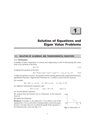
  • 1. 1 Solution of Equations and Eigen Value Problems 1.1 SOLUTION OF ALGEBRAIC AND TRANSCENDENTAL EQUATIONS 1.1.1 Introduction A problem of great importance in science and engineering is that of determining the roots/ zeros of an equation of the form f(x) = 0, (1.1) A polynomial equation of the form f(x) = Pn(x) = a0xn + a1xn–1 + a2xn–2 + ... + an –1x + an = 0 (1.2) is called analgebraic equation. An equation which contains polynomials, exponential functions, logarithmic functions, trigonometric functions etc. is called a transcendental equation. For example, 3x3 – 2x2 – x – 5 = 0, x4 – 3x2 + 1 = 0, x2 – 3x + 1 = 0, are algebraic (polynomial) equations, and xe2x – 1 = 0, cos x – xex = 0, tan x = x are transcendental equations. We assume that the function f(x) is continuous in the required interval. We define the following. Root/zero A number α, for which f(α) ≡ 0 is called a root of the equation f(x) = 0, or a zero of f(x). Geometrically, a root of an equa- tion f(x) = 0 is the value of x at which the graph of the equation y = f(x) intersects the x-axis (see Fig. 1.1). f(x) O x Fig. 1.1 ‘Root of f(x) = 0’
  • 2. 2 NUMERICAL METHODS Simple root A number α is a simple root of f(x) = 0, if f(α) = 0 and f ′(α) ≠ 0. Then, we can write f(x) as f(x) = (x – α) g(x), g(α) ≠ 0. (1.3) For example, since (x – 1) is a factor of f(x) = x3 + x – 2 = 0, we can write f(x) = (x – 1)(x2 + x + 2) = (x – 1) g(x), g(1) ≠ 0. Alternately, we find f(1) = 0, f ′(x) = 3x2 + 1, f ′(1) = 4 ≠ 0. Hence, x = 1 is a simple root of f(x) = x3 + x – 2 = 0. Multiple root A number α is a multiple root, of multiplicity m, of f(x) = 0, if f(α) = 0, f ′(α) = 0, ..., f (m –1) (α) = 0, and f (m) (α) ≠ 0. (1.4) Then, we can write f(x) as f(x) = (x – α)m g(x), g(α) ≠ 0. For example, consider the equation f(x) = x3 – 3x2 + 4 = 0. We find f(2) = 8 – 12 + 4 = 0, f ′(x) = 3x2 – 6x, f ′(2) = 12 – 12 = 0, f ″(x) = 6x – 6, f ″(2) = 6 ≠ 0. Hence, x = 2 is a multiple root of multiplicity 2 (double root) of f(x) = x3 – 3x2 + 4 = 0. We can write f(x) = (x – 2)2 (x + 1) = (x – 2)2 g(x), g(2) = 3 ≠ 0. In this chapter, we shall be considering the case of simple roots only. Remark 1 A polynomial equation of degree n has exactly n roots, real or complex, simple or multiple, where as a transcendental equation may have one root, infinite number of roots or no root. We shall derive methods for finding only the real roots. The methods for finding the roots are classified as (i) direct methods, and (ii) iterative methods. Direct methods These methods give the exact values of all the roots in a finite number of steps (disregarding the round-off errors). Therefore, for any direct method, we can give the total number of operations (additions, subtractions, divisions and multiplications). This number is called the operational count of the method. For example, the roots of the quadratic equation ax2 + bx + c = 0, a ≠ 0, can be obtained using the method x = 1 2 4 2 a b b ac − ± − L N M O Q P. For this method, we can give the count of the total number of operations. There are direct methods for finding all the roots of cubic and fourth degree polynomi- als. However, these methods are difficult to use. Direct methods for finding the roots of polynomial equations of degree greater than 4 or transcendental equations are not available in literature.
  • 3. SOLUTION OF EQUATIONS AND EIGEN VALUE PROBLEMS 3 Iterative methods These methods are based on the idea of successive approximations. We start with one or two initial approximations to the root and obtain a sequence of approxima- tions x0, x1, ..., xk, ..., which in the limit as k → ∞, converge to the exact root α. An iterative method for finding a root of the equation f(x) = 0 can be obtained as xk + 1 = φ(xk), k = 0, 1, 2, ..... (1.5) This method uses one initial approximation to the root . 0 x The sequence of approxima- tions is given by x1 = φ(x0), x2 = φ(x1), x3 = φ(x2), ..... The function φ is called an iteration function and x0 is called an initial approximation. If a method uses two initial approximations x0, x1, to the root, then we can write the method as xk + 1 = φ(xk – 1, xk), k = 1, 2, ..... (1.6) Convergence of iterative methods The sequence of iterates, {xk}, is said to converge to the exact root α, if lim k → ∞ xk = α, or lim k → ∞ | xk – α | = 0. (1.7) The error of approximation at the kth iterate is defined as εk = xk – α. Then, we can write (1.7) as lim k → ∞ | error of approximation | = lim k → ∞ | xk – α | = lim k → ∞ | εk | = 0. Remark 2 Given one or two initial approximations to the root, we require a suitable iteration function φ for a given function f(x), such that the sequence of iterates, {xk}, converge to the exact root α. Further, we also require a suitable criterion to terminate the iteration. Criterion to terminate iteration procedure Since, we cannot perform infinite number of iterations, we need a criterion to stop the iterations. We use one or both of the following criterion: (i) The equation f(x) = 0 is satisfied to a given accuracy or f(xk) is bounded by an error tolerance ε. | f (xk) | ≤ ε. (1.8) (ii) The magnitude of the difference between two successive iterates is smaller than a given accuracy or an error bound ε. | xk + 1 – xk | ≤ ε. (1.9) Generally, we use the second criterion. In some very special problems, we require to use both the criteria. For example, if we require two decimal place accuracy, then we iterate until | xk+1 – xk | 0.005. If we require three decimal place accuracy, then we iterate until | xk+1 – xk | 0.0005. As we have seen earlier, we require a suitable iteration function and suitable initial approximation(s) to start the iteration procedure. In the next section, we give a method to find initial approximation(s).
  • 4. 4 NUMERICAL METHODS 1.1.2 Initial Approximation for an Iterative Procedure For polynomial equations, Descartes’ rule of signs gives the bound for the number of positive and negative real roots. (i) We count the number of changes of signs in the coefficients of Pn(x) for the equation f(x) = Pn(x) = 0. The number of positive roots cannot exceed the number of changes of signs. For example, if there are four changes in signs, then the equation may have four positive roots or two positive roots or no positive root. If there are three changes in signs, then the equation may have three positive roots or definitely one positive root. (For polynomial equations with real coefficients, complex roots occur in conjugate pairs.) (ii) We write the equation f(– x) = Pn(– x) = 0, and count the number of changes of signs in the coefficients of Pn(– x). The number of negative roots cannot exceed the number of changes of signs. Again, if there are four changes in signs, then the equation may have four negative roots or two negative roots or no negative root. If there are three changes in signs, then the equation may have three negative roots or definitely one negative root. We use the following theorem of calculus to determine an initial approximation. It is also called the intermediate value theorem. Theorem 1.1 If f(x) is continuous on some interval [a, b] and f(a)f(b) 0, then the equation f(x) = 0 has at least one real root or an odd number of real roots in the interval (a, b). This result is very simple to use. We set up a table of values of f (x) for various values of x. Studying the changes in signs in the values of f (x), we determine the intervals in which the roots lie. For example, if f (1) and f (2) are of opposite signs, then there is a root in the interval (1, 2). Let us illustrate through the following examples. Example 1.1 Determine the maximum number of positive and negative roots and intervals of length one unit in which the real roots lie for the following equations. (i) 8x3 – 12x2 – 2x + 3 = 0 (ii) 3x3 – 2x2 – x – 5 = 0. Solution (i) Let f(x) = 8x3 – 12x2 – 2x + 3 = 0. The number of changes in the signs of the coefficients (8, – 12, – 2, 3) is 2. Therefore, the equation has 2 or no positive roots. Now, f(– x) = – 8x3 – 12x2 + 2x + 3. The number of changes in signs in the coefficients (– 8, – 12, 2, 3) is 1. Therefore, the equation has one negative root. We have the following table of values for f(x), (Table 1.1). Table 1.1. Values of f (x), Example 1.1(i). x – 2 – 1 0 1 2 3 f(x) – 105 – 15 3 – 3 15 105 Since f(– 1) f(0) 0, there is a root in the interval (– 1, 0), f(0) f(1) 0, there is a root in the interval (0, 1), f(1) f(2) 0, there is a root in the interval (1, 2).
  • 5. SOLUTION OF EQUATIONS AND EIGEN VALUE PROBLEMS 5 Therefore, there are three real roots and the roots lie in the intervals (– 1, 0), (0, 1), (1, 2). (ii) Let f(x) = 3x2 – 2x2 – x – 5 = 0. The number of changes in the signs of the coefficients (3, – 2, – 1, – 5) is 1. Therefore, the equation has one positive root. Now, f(– x) = – 3x2 – 2x2 + x – 5. The number of changes in signs in the coefficients (– 3, – 2, 1, – 5) is 2. Therefore, the equation has two negative or no negative roots. We have the table of values for f (x), (Table 1.2). Table 1.2. Values of f (x ), Example 1.1(ii). x – 3 – 2 – 1 0 1 2 3 f(x) – 101 – 35 – 9 – 5 – 5 9 55 From the table, we find that there is one real positive root in the interval (1, 2). The equation has no negative real root. Example 1.2 Determine an interval of length one unit in which the negative real root, which is smallest in magnitude lies for the equation 9x3 + 18x2 – 37x – 70 = 0. Solution Let f(x) = 9x3 + 18x2 – 37x – 70 = 0. Since, the smallest negative real root in magni- tude is required, we form a table of values for x 0, (Table 1.3). Table 1.3. Values of f (x ), Example 1.2. x – 5 – 4 – 3 – 2 – 1 0 f(x) – 560 – 210 – 40 4 – 24 – 70 Since, f(– 2)f(– 1) 0, the negative root of smallest magnitude lies in the interval (– 2, –1). Example 1.3 Locate the smallest positive root of the equations (i) xex = cos x. (ii) tan x = 2x. Solution (i) Let f(x) = xex – cos x = 0. We have f(0) = – 1, f(1) = e – cos 1 = 2.718 – 0.540 = 2.178. Since, f(0) f(1) 0, there is a root in the interval (0, 1). (ii) Let f(x) = tan x – 2x = 0. We have the following function values. f(0) = 0, f(0.1) = – 0.0997, f(0.5) = – 0.4537, f(1) = – 0.4426, f(1, 1) = – 0.2352, f(1.2) = 0.1722. Since, f(1.1) f(1.2) 0, the root lies in the interval (1.1, 1.2). Now, we present some iterative methods for finding a root of the given algebraic or transcendental equation. We know from calculus, that in the neighborhood of a point on a curve, the curve can be approximated by a straight line. For deriving numerical methods to find a root of an equation
  • 6. 6 NUMERICAL METHODS f(x) = 0, we approximate the curve in a sufficiently small interval which contains the root, by a straight line. That is, in the neighborhood of a root, we approximate f(x) ≈ ax + b, a ≠ 0 where a and b are arbitrary parameters to be determined by prescribing two appropriate conditions on f(x) and/or its derivatives. Setting ax + b = 0, we get the next approximation to the root as x = – b/a. Different ways of approximating the curve by a straight line give different methods. These methods are also called chord methods. Method of false position (also called regula-falsi method) and Newton-Raphson method fall in this category of chord methods. 1.1.3 Method of False Position The method is also called linear interpolation method or chord method or regula-falsi method. At the start of all iterations of the method, we require the interval in which the root lies. Let the root of the equation f(x) = 0, lie in the interval (xk–1, xk), that is, fk–1 fk 0, where f(xk–1) = fk–1, and f(xk) = fk. Then, P(xk–1, fk–1), Q(xk, fk) are points on the curve f(x) = 0. Draw a straight line joining the points P and Q (Figs. 1.2a, b). The line PQ is taken as an approxima- tion of the curve in the interval [xk–1, xk]. The equation of the line PQ is given by y f f f x x x x k k k k k k − − = − − − − 1 1 . The point of intersection of this line PQ with the x-axis is taken as the next approxima- tion to the root. Setting y = 0, and solving for x, we get x = xk – x x f f k k k k − − − − F HG I KJ 1 1 fk = xk – x x f f k k k k − − F HG I KJ − − 1 1 fk. The next approximation to the root is taken as xk+1 = xk – x x f f k k k k − − F HG I KJ − − 1 1 fk. (1.10) Simplifying, we can also write the approximation as xk+1 = x f f x x f f f k k k k k k k k ( ) ( ) − − − − − − − 1 1 1 = x f x f f f k k k k k k − − − − − 1 1 1 , k = 1, 2, ... (1.11) Therefore, starting with the initial interval (x0, x1), in which the root lies, we compute x2 = x f x f f f 0 1 1 0 1 0 − − . Now, if f(x0) f(x2) 0, then the root lies in the interval (x0, x2). Otherwise, the root lies in the interval (x2, x1). The iteration is continued using the interval in which the root lies, until the required accuracy criterion given in Eq.(1.8) or Eq.(1.9) is satisfied. Alternate derivation of the method Let the root of the equation f(x) = 0, lie in the interval (xk–1, xk). Then, P(xk–1, fk–1), Q(xk, fk) are points on the curve f(x) = 0. Draw the chord joining the points P and Q (Figs. 1.2a, b). We
  • 7. SOLUTION OF EQUATIONS AND EIGEN VALUE PROBLEMS 7 approximate the curve in this interval by the chord, that is, f(x) ≈ ax + b. The next approximation to the root is given by x = – b/a. Since the chord passes through the points P and Q, we get fk–1 = axk–1 + b, and fk = axk + b. Subtracting the two equations, we get fk – fk–1 = a(xk – xk – 1), or a = f f x x k k k k − − − − 1 1 . The second equation gives b = fk – axk. Hence, the next approximation is given by xk+1 = – b a f ax a k k = − − = xk – f a k = xk – x x f f k k k k − − F HG I KJ − − 1 1 fk which is same as the method given in Eq.(1.10). y O x P x3 x2 x1 x0 Q y O x P x3 x2 x1 x0 Q Fig. 1.2a ‘Method of false position’ Fig. 1.2b ‘Method of false position’ Remark 3 At the start of each iteration, the required root lies in an interval, whose length is decreasing. Hence, the method always converges. Remark 4 The method of false position has a disadvantage. If the root lies initially in the interval (x0, x1), then one of the end points is fixed for all iterations. For example, in Fig.1.2a, the left end point x0 is fixed and the right end point moves towards the required root. There- fore, in actual computations, the method behaves like xk+1 = x f x f f f k k k 0 0 0 − − , k = 1, 2, … (1.12) In Fig.1.2b, the right end point x1 is fixed and the left end point moves towards the required root. Therefore, in this case, in actual computations, the method behaves like xk+1 = x f x f f f k k k 1 1 1 − − , k = 1, 2, … (1.13) Remark 5 The computational cost of the method is one evaluation of the function f(x), for each iteration. Remark 6 We would like to know why the method is also called a linear interpolation method. Graphically, a linear interpolation polynomial describes a straight line or a chord. The linear interpolation polynomial that fits the data (xk–1, fk–1), (xk, fk) is given by
  • 8. 8 NUMERICAL METHODS f(x) = x x x x k k k − − −1 fk–1 + x x x x k k k − − − − 1 1 fk. (We shall be discussing the concept of interpolation polynomials in Chapter 2). Setting f(x) = 0, we get ( ) ( ) x x f x x f x x k k k k k k − − − − − − − 1 1 1 = 0, or x(fk – fk–1) = xk–1 fk – xk fk – 1 or x = xk+1 = x f x f f f k k k k k k − − − − − 1 1 1 . This gives the next approximation as given in Eq. (1.11). Example 1.4 Locate the intervals which contain the positive real roots of the equation x3 – 3x + 1 = 0. Obtain these roots correct to three decimal places, using the method of false position. Solution We form the following table of values for the function f(x). x 0 1 2 3 f (x) 1 – 1 3 19 There is one positive real root in the interval (0, 1) and another in the interval (1, 2). There is no real root for x 2 as f(x) 0, for all x 2. First, we find the root in (0, 1). We have x0 = 0, x1 = 1, f0 = f(x0) = f(0) = 1, f1 = f(x1) = f(1) = – 1. x2 = x f x f f f 0 1 1 0 1 0 0 1 1 1 − − = − − − = 0.5, f(x2) = f(0.5) = – 0.375. Since, f(0) f(0.5) 0, the root lies in the interval (0, 0.5). x3 = x f x f f f 0 2 2 0 2 0 0 0 5 1 0 375 1 − − = − − − . ( ) . = 0.36364, f(x3) = f(0.36364) = – 0.04283. Since, f(0) f(0.36364) 0, the root lies in the interval (0, 0.36364). x4 = x f x f f f 0 3 3 0 3 0 0 036364 1 0 04283 1 − − = − − − . ( ) . = 0.34870,f(x4) = f(0.34870) = – 0.00370. Since, f(0) f(0.3487) 0, the root lies in the interval (0, 0.34870). x5 = x f x f f f 0 4 4 0 4 0 0 03487 1 0 00370 1 − − = − − − . ( ) . = 0.34741, f(x5) = f(0.34741) = – 0.00030. Since, f(0) f(0.34741) 0, the root lies in the interval (0, 0.34741). x6 = x f x f f f 0 5 5 0 5 0 0 034741 1 0 0003 1 − − = − − − . ( ) . = 0.347306.
  • 9. SOLUTION OF EQUATIONS AND EIGEN VALUE PROBLEMS 9 Now, | x6 – x5 | = | 0.347306 – 0.34741 | ≈ 0.0001 0.0005. The root has been computed correct to three decimal places. The required root can be taken as x ≈ x6 = 0.347306. We may also give the result as 0.347, even though x6 is more accurate. Note that the left end point x = 0 is fixed for all iterations. Now, we compute the root in (1, 2). We have x0 = 1, x1 = 2, f0 = f(x0) = f(1) = – 1, f1 = f(x1) = f(2) = 3. x2 = x f x f f f 0 1 1 0 1 0 3 2 1 3 1 − − = − − − − ( ) ( ) = 1.25, f(x2) = f(1.25) = – 0.796875. Since, f(1.25)f(2) 0, the root lies in the interval (1.25, 2). We use the formula given in Eq.(1.13). x3 = x f x f f f 2 1 1 2 1 2 − − = − − − − 1.25(3) 2( 0.796875) 3 ( 0.796875) = 1.407407, f(x3) = f(1.407407) = – 0.434437. Since, f(1.407407) f(2) 0, the root lies in the interval (1.407407, 2). x4 = x f x f f f 3 1 1 3 1 3 − − = − − − − 1.407407(3) 2( 0.434437) 3 ( 0.434437) = 1.482367, f(x4) = f(1.482367) = – 0.189730. Since f(1.482367) f(2) 0, the root lies in the interval (1.482367, 2). x5 = x f x f f f 4 1 1 4 1 4 − − = − − − − 1.482367(3) 2( 0.18973) 3 ( 0.18973) = 1.513156, f(x5) = f(1.513156) = – 0.074884. Since, f(1.513156) f(2) 0, the root lies in the interval (1.513156, 2). x6 = x f x f f f 5 1 1 5 1 5 − − = − − − − 1.513156(3) 2( 0.074884) 3 ( 0.74884) = 1.525012, f(x6) = f(1.525012) = – 0.028374. Since, f(1.525012) f(2) 0, the root lies in the interval (1.525012, 2). x7 = x f x f f f 6 1 1 6 1 6 − − = − − − − 1.525012(3) 2( 0.028374) 3 ( 0.028374) = 1.529462. f(x7) = f(1.529462) = – 0.010586. Since, f(1.529462) f(2) 0, the root lies in the interval (1.529462, 2). x8 = x f x f f f 7 1 1 7 1 7 − − = − − − − 1.529462(3) 2( 0.010586) 3 ( 0.010586) = 1.531116, f(x8) = f(1.531116) = – 0.003928. Since, f(1.531116) f(2) 0, the root lies in the interval (1.531116, 2).
  • 10. 10 NUMERICAL METHODS x9 = x f x f f f 8 1 1 8 1 8 − − = − − − − 1.531116(3) 2( 0.003928) 3 ( 0.003928) = 1.531729, f(x9) = f(1.531729) = – 0.001454. Since, f(1.531729) f(2) 0, the root lies in the interval (1.531729, 2). x10 = x f x f f f 9 1 1 9 1 9 − − = − − − − 1.531729(3) 2( 0.001454) 3 ( 0.001454) = 1.531956. Now, |x10 – x9 | = | 1.531956 – 1.53179 | ≈ 0.000227 0.0005. The root has been computed correct to three decimal places. The required root can be taken as x ≈ x10 = 1.531956. Note that the right end point x = 2 is fixed for all iterations. Example 1.5 Find the root correct to two decimal places of the equation xex = cos x, using the method of false position. Solution Define f(x) = cos x – xex = 0. There is no negative root for the equation. We have f(0) = 1, f(1) = cos 1 – e = – 2.17798. A root of the equation lies in the interval (0, 1). Let x0 = 0, x1 = 1. Using the method of false position, we obtain the following results. x2 = x f x f f f 0 1 1 0 1 0 − − = − − − 0 1(1) 2.17798 1 = 0.31467, f(x2) = f(0.31467) = 0.51986. Since, f(0.31467) f(1) 0, the root lies in the interval (0.31467, 1). We use the formula given in Eq.(1.13). x3 = x f x f f f 2 1 1 2 1 2 − − = − − − − 0.31467( 2.17798) 1(0.51986) 2.17798 0.51986 = 0.44673, f(x3) = f(0.44673) = 0.20354. Since, f(0.44673) f(1) 0, the root lies in the interval (0.44673, 1). x4 = x f x f f f 3 1 1 3 1 3 − − = − − − − 0.44673( 2.17798) 1(0.20354) 2.17798 0.20354 = 0.49402, f(x4) = f(0.49402) = 0.07079. Since, f(0.49402) f(1) 0, the root lies in the interval (0.49402, 1). x5 = x f x f f f 4 1 1 4 1 4 − − = − − − − 0 . 49402( 2.17798) 1(0.07079) 2.17798 0.07079 = 0.50995, f(x5) = f(0.50995) = 0.02360. Since, f(0.50995) f(1) 0, the root lies in the interval (0.50995, 1). x6 = x f x f f f 5 1 1 5 1 5 − − = − − − − 0.50995( 2.17798) 1(0.0236) 2.17798 0.0236 = 0.51520, f(x6) = f(0.51520) = 0.00776.
  • 11. SOLUTION OF EQUATIONS AND EIGEN VALUE PROBLEMS 11 Since, f(0.51520) f(1) 0, the root lies in the interval (0.51520, 1). x7 = x f x f f f 6 1 1 6 1 6 − − = − − − − 0.5152( 2.17798) 1(0.00776) 2.17798 0.00776 = 0.51692. Now, | x7 – x6 | = | 0.51692 – 0.51520 | ≈ 0.00172 0.005. The root has been computed correct to two decimal places. The required root can be taken as x ≈ x7 = 0.51692. Note that the right end point x = 2 is fixed for all iterations. 1.1.4 Newton-Raphson Method This method is also called Newton’s method. This method is also a chord method in which we approximate the curve near a root, by a straight line. Let 0 x be an initial approximation to the root of f(x) = 0. Then, P(x0, f0), where f0 = f(x0), is a point on the curve. Draw the tangent to the curve at P, (Fig. 1.3). We approximate the curve in the neighborhood of the root by the tangent to the curve at the point P. The point of intersection of the tangent with the x-axis is taken as the next approximation to the root. The process is repeated until the required accuracy is obtained. The equation of the tangent to the curve y = f(x) at the point P(x0, f0) is given by y – f(x0) = (x – x0) f ′(x0) where f ′(x0) is the slope of the tangent to the curve at P. Setting y = 0 and solving for x, we get x = x0 – f x f x ( ) ( ) 0 0 ′ , f ′(x0) ≠ 0. The next approximation to the root is given by x1 = x0 – f x f x ( ) ( ) 0 0 ′ , f ′(x0) ≠ 0. We repeat the procedure. The iteration method is defined as xk+1 = xk – f x f x k k ( ) ( ) ′ , f ′(xk) ≠ 0. (1.14) This method is called the Newton-Raphson method or simply the Newton’s method. The method is also called the tangent method. Alternate derivation of the method Let xk be an approximation to the root of the equation f(x) = 0. Let ∆x be an increment in x such that xk + ∆x is the exact root, that is f(xk + ∆x) ≡ 0. y O x P x1 x0 Fig. 1.3 ‘Newton-Raphson method’
  • 12. 12 NUMERICAL METHODS Expanding in Taylor’s series about the point xk, we get f(xk) + ∆x f ′(xk) + ( ) ! ∆x 2 2 f ″ (xk) + ... = 0. (1.15) Neglecting the second and higher powers of ∆x, we obtain f(xk) + ∆x f ′(xk) ≈ 0, or ∆x = – f x f x k k ( ) ( ) ′ . Hence, we obtain the iteration method xk+1 = xk + ∆x = xk – f x f x k k ( ) ( ) ′ , f ′(xk) ≠ 0, k = 0, 1, 2, ... which is same as the method derived earlier. Remark 7 Convergence of the Newton’s method depends on the initial approximation to the root. If the approximation is far away from the exact root, the method diverges (see Example 1.6). However, if a root lies in a small interval (a, b) and x0 ∈ (a, b), then the method converges. Remark 8 From Eq.(1.14), we observe that the method may fail when f ′(x) is close to zero in the neighborhood of the root. Later, in this section, we shall give the condition for convergence of the method. Remark 9 The computational cost of the method is one evaluation of the function f(x) and one evaluation of the derivative f ′(x), for each iteration. Example 1.6 Derive the Newton’s method for finding 1/N, where N 0. Hence, find 1/17, using the initial approximation as (i) 0.05, (ii) 0.15. Do the iterations converge ? Solution Let x = 1 N , or 1 x = N. Define f(x) = 1 x – N. Then, f ′(x) = – 1 2 x . Newton’s method gives xk+1 = xk – f x f x k k ( ) ( ) ′ = xk – [( / ) ] [ / ] 1 1 2 x N x k k − − = xk + [xk – Nxk 2 ] = 2xk – Nxk 2 . (i) With N = 17, and x0 = 0.05, we obtain the sequence of approximations x1 = 2x0 – Nx0 2 = 2(0.05) – 17(0.05)2 = 0.0575. x2 = 2x1 – Nx1 2 = 2(0.0575) – 17(0.0575)2 = 0.058794. x3 = 2x2 – Nx2 2 = 2(0.058794) – 17(0.058794)2 = 0.058823. x4 = 2x3 – Nx3 2 = 2(0.058823) – 17(0.058823)2 = 0.058823. Since, | x4 – x3 | = 0, the iterations converge to the root. The required root is 0.058823. (ii) With N = 17, and x0 = 0.15, we obtain the sequence of approximations x1 = 2x0 – Nx0 2 = 2(0.15) – 17(0.15)2 = – 0.0825.
  • 13. SOLUTION OF EQUATIONS AND EIGEN VALUE PROBLEMS 13 x2 = 2x1 – Nx1 2 = 2(– 0.0825) – 17(– 0.8025)2 = – 0.280706. x3 = 2x2 – Nx2 2 = 2(– 0.280706) – 17(– 0.280706)2 = – 1.900942. x4 = 2x3 – Nx3 2 = 2(– 1.900942) – 17(– 1.900942)2 = – 65.23275. We find that xk → – ∞ as k increases. Therefore, the iterations diverge very fast. This shows the importance of choosing a proper initial approximation. Example 1.7 Derive the Newton’s method for finding the qth root of a positive number N, N1/q, where N 0, q 0. Hence, compute 171/3 correct to four decimal places, assuming the initial approximation as x0 = 2. Solution Let x = N1/q, or xq = N. Define f(x) = xq – N. Then, f ′(x) = qxq – 1. Newton’s method gives the iteration xk+1 = xk – x N qx qx x N qx q x N qx k q k q k q k q k q k q k q − = − + = − + − − − 1 1 1 1 ( ) . For computing 171/3, we have q = 3 and N = 17. Hence, the method becomes xk+1 = 2 17 3 3 2 x x k k + , k = 0, 1, 2, ... With x0 = 2, we obtain the following results. x1 = 2 17 3 2 8 17 3 4 0 3 0 2 x x + = + ( ) ( ) = 2.75, x2 = 2 17 3 1 3 1 2 x x + = + 2(2.75) 17 3(2.75) 3 2 = 2.582645, x3 = 2 17 3 2 3 2 2 x x + = + 2(2.582645) 17 3(2.582645) 3 2 = 2.571332, x4 = 2 17 3 3 3 3 2 x x + = + 2(2.571332) 17 3(2.571332) 3 2 = 2.571282. Now, | x4 – x3 | = | 2.571282 – 2.571332 | = 0.00005. We may take x ≈ 2.571282 as the required root correct to four decimal places. Example 1.8 Perform four iterations of the Newton’s method to find the smallest positive root of the equation f(x) = x3 – 5x + 1 = 0. Solution We have f(0) = 1, f(1) = – 3. Since, f(0) f(1) 0, the smallest positive root lies in the interval (0, 1). Applying the Newton’s method, we obtain xk+1 = xk – x x x x x k k k k k 3 2 3 2 5 1 3 5 2 1 3 5 − + − = − − , k = 0, 1, 2, ...
  • 14. 14 NUMERICAL METHODS Let x0 = 0.5. We have the following results. x1 = 2 1 3 5 2 0 5 1 3 0 5 5 0 3 0 2 3 2 x x − − = − − ( . ) ( . ) = 0.176471, x2 = 2 1 3 5 2 0 176471 1 3 0 176471 5 1 3 1 2 3 2 x x − − = − − ( . ) ( . ) = 0.201568, x3 = 2 1 3 5 2 0 201568 1 3 0 201568 5 2 3 2 2 3 2 x x − − = − − ( . ) ( . ) = 0.201640, x4 = 2 1 3 5 2 0 201640 1 3 0 201640 5 3 3 3 2 3 2 x x − − = − − ( . ) ( . ) = 0.201640. Therefore, the root correct to six decimal places is x ≈ 0.201640. Example 1.9 Using Newton-Raphson method solve x log10 x = 12.34 with x0 = 10. (A.U. Apr/May 2004) Solution Define f(x) = x log10 x – 12.34. Then f ′(x) = log10 x + 1 10 loge = log10 x + 0.434294. Using the Newton-Raphson method, we obtain xk+1 = xk – x x x k k k log . log . 10 10 12 34 0 434294 − + , k = 0, 1, 2, ... With x0 = 10, we obtain the following results. x1 = x0 – x x x 0 10 0 10 0 log 12.34 log 0.434294 − + = 10 – 10 10 10 10 10 log log − + 12.34 0.434294 = 11.631465. x2 = x1 – x x x 1 10 1 10 1 log log − + 12.34 0.434294 = 11.631465 – 11.631465 11.631465 11.631465 10 10 log log − + 12.34 0.434294 = 11.594870. x3 = x2 – x x x 2 10 2 10 2 log log − + 12.34 0.434294 = 11.59487 – 11.59487 11.59487 12.34 11.59487 0.434294 log log 10 10 − + = 11.594854. We have | x3 – x2 | = | 11.594854 – 11.594870 | = 0.000016. We may take x ≈ 11.594854 as the root correct to four decimal places.
  • 15. SOLUTION OF EQUATIONS AND EIGEN VALUE PROBLEMS 15 1.1.5 General Iteration Method The method is also called iteration method or method of successive approximations or fixed point iteration method. The first step in this method is to rewrite the given equation f(x) = 0 in an equivalent form as x = φ(x). (1.16) There are many ways of rewriting f(x) = 0 in this form. For example, f(x) = x3 – 5x + 1 = 0, can be rewritten in the following forms. x = x3 1 5 + , x = (5x – 1)1/3, x = 5 1 x x − , etc. (1.17) Now, finding a root of f(x) = 0 is same as finding a number α such that α = φ(α), that is, a fixed point of φ(x). A fixed point of a function φ is a point α such that α = φ(α). This result is also called the fixed point theorem. Using Eq.(1.16), the iteration method is written as xk+1 = φ(xk), k = 0, 1, 2, ... (1.18) The function φ(x) is called the iteration function. Starting with the initial approxima- tion x0, we compute the next approximations as x1 = φ(x0), x2 = φ(x1), x3 = φ(x2),... The stopping criterion is same as used earlier. Since, there are many ways of writing f(x) = 0 as x = φ(x), it is important to know whether all or at least one of these iteration methods converges. Remark 10 Convergence of an iteration method xk+1 = φ(xk), k = 0, 1, 2,..., depends on the choice of the iteration function φ(x), and a suitable initial approximation x0, to the root. Consider again, the iteration methods given in Eq.(1.17), for finding a root of the equation f(x) = x3 – 5x + 1 = 0. The positive root lies in the interval (0, 1). (i) xk+1 = xk 3 1 5 + , k = 0, 1, 2, ... (1.19) With x0 = 1, we get the sequence of approximations as x1 = 0.4, x2 = 0.2128, x3 = 0.20193, x4 = 0.20165, x5 = 0.20164. The method converges and x ≈ x5 = 0.20164 is taken as the required approximation to the root. (ii) xk+1 = (5xk – 1)1/3, k = 0, 1, 2, ... (1.20) With x0 = 1, we get the sequence of approximations as x1 = 1.5874, x2 = 1.9072, x3 = 2.0437, x4 = 2.0968,... which does not converge to the root in (0, 1). (iii) xk+1 = 5 1 x x k k − , k = 0, 1, 2, ... (1.21)
  • 16. 16 NUMERICAL METHODS With x0 = 1, we get the sequence of approximations as x1 = 2.0, x2 = 2.1213, x3 = 2.1280, x4 = 2.1284,... which does not converge to the root in (0, 1). Now, we derive the condition that the iteration function φ(x) should satisfy in order that the method converges. Condition of convergence The iteration method for finding a root of f(x) = 0, is written as xk+1 = φ(xk), k = 0, 1, 2,... (1.22) Let α be the exact root. That is, α = φ(α). (1.23) We define the error of approximation at the kth iterate as εk = xk – α, k = 0, 1, 2,... Subtracting (1.23) from (1.22), we obtain xk+1 – α = φ(xk) – φ(α) = (xk – α)φ′(tk) (using the mean value theorem) (1.24) or εk+1 = φ′(tk) εk, xk tk α. Setting k = k – 1, we get εk = φ′(tk–1) εk–1, xk–1 tk–1 α. Hence, εk+1 = φ′(tk)φ′(tk–1) εk–1. Using (1.24) recursively, we get εk+1 = φ′(tk)φ′(tk–1) ... φ′(t0) ε0. The initial error ε0 is known and is a constant. We have | εk+1 | = | φ′(tk) | | φ′(tk–1) | ... | φ′(t0) | | ε0 |. Let | φ′(tk) | ≤ c, k = 0, 1, 2,… Then, | εk+1 | ≤ ck+1 | ε0 |. (1.25) For convergence, we require that | εk+1 | → 0 as k → ∞. This result is possible, if and only if c 1. Therefore, the iteration method (1.22) converges, if and only if | φ′(xk) | ≤ c 1, k = 0, 1, 2, ... or | φ′(x) | ≤ c 1, for all x in the interval (a, b). (1.26) We can test this condition using x0, the initial approximation, before the computations are done. Let us now check whether the methods (1.19), (1.20), (1.21) converge to a root in (0, 1) of the equation f(x) = x3 – 5x + 1 = 0. (i) We have φ(x) = x3 1 5 + , φ′(x) = 3 5 2 x , and | φ′(x) | = 3 5 2 x ≤ 1 for all x in . 1 0 x Hence, the method converges to a root in (0, 1).
  • 17. SOLUTION OF EQUATIONS AND EIGEN VALUE PROBLEMS 17 (ii) We have φ(x) = (5x – 1)1/3, φ′(x) = 5 3 5 1 2 3 ( ) / x − . Now | φ′(x) | 1, when x is close to 1 and | φ′(x) | 1 in the other part of the interval. Convergence is not guaranteed. (iii) We have φ(x) = 5 1 x x − , φ′(x) = 1 2 5 1 3 2 1 2 x x / / ( ) − . Again, | φ′(x) | 1, when x is close to 1 and | φ′(x) | 1 in the other part of the interval. Convergence is not guaranteed. Remark 11 Sometimes, it may not be possible to find a suitable iteration function φ(x) by manipulating the given function f(x). Then, we may use the following procedure. Write f(x) = 0 as x = x + α f(x) = φ(x), where α is a constant to be determined. Let x0 be an initial approximation contained in the interval in which the root lies. For convergence, we require | φ′(x0) | = | 1 + α f′(x0) | 1. (1.27) Simplifying, we find the interval in which α lies. We choose a value for α from this interval and compute the approximations. A judicious choice of a value in this interval may give faster convergence. Example 1.10 Find the smallest positive root of the equation x3 – x – 10 = 0, using the general iteration method. Solution We have f(x) = x3 – x – 10, f(0) = – 10, f(1) = – 10, f(2) = 8 – 2 – 10 = – 4, f(3) = 27 – 3 – 10 = 14. Since, f(2) f(3) 0, the smallest positive root lies in the interval (2, 3). Write x3 = x + 10, and x = (x + 10)1/3 = φ(x). We define the iteration method as xk+1 = (xk + 10)1/3. We obtain φ′(x) = 1 3 10 2 3 ( ) / x + . We find | φ′(x) | 1 for all x in the interval (2, 3). Hence, the iteration converges. Let x0 = 2.5. We obtain the following results. x1 = (12.5)1/3 = 2.3208, x2 = (12.3208)1/3 = 2.3097, x3 = (12.3097)1/3 = 2.3090, x4 = (12.3090)1/3 = 2.3089. Since, | x4 – x3 | = 2.3089 – 2.3090 | = 0.0001, we take the required root as x ≈ 2.3089. Example 1.11 Find the smallest negative root in magnitude of the equation 3x4 + x3 + 12x + 4 = 0, using the method of successive approximations. Solution We have f(x) = 3x4 + x3 + 12x + 4 = 0, f(0) = 4, f(– 1) = 3 – 1 – 12 + 4 = – 6. Since, f(– 1) f(0) 0, the smallest negative root in magnitude lies in the interval (– 1, 0).
  • 18. 18 NUMERICAL METHODS Write the given equation as x(3x3 + x2 + 12) + 4 = 0, and x = – 4 3 12 3 2 x x + + = φ(x). The iteration method is written as xk+1 = – 4 3 12 3 2 x x k k + + . We obtain φ′(x) = 4 9 2 3 12 2 3 2 2 ( ) ( ) x x x x + + + . We find | φ′(x) | 1 for all x in the interval (– 1, 0). Hence, the iteration converges. Let x0 = – 0.25. We obtain the following results. x1 = – 4 3 0 25 0 25 12 3 2 ( . ) ( . ) − + − + = – 0.33290, x2 = – 4 3 0 3329 0 3329 12 3 2 ( . ) ( . ) − + − + = – 0.33333, x3 = – 4 3 0 33333 0 33333 12 3 2 ( . ) ( . ) − + − + = – 0.33333. The required approximation to the root is x ≈ – 0.33333. Example 1.12 The equation f(x) = 3x3 + 4x2 + 4x + 1 = 0 has a root in the interval (– 1, 0). Determine an iteration function φ(x), such that the sequence of iterations obtained from xk+1 = φ(xk), x0 = – 0.5, k = 0, 1,..., converges to the root. Solution We illustrate the method given in Remark 10. We write the given equation as x = x + α (3x3 + 4x2 + 4x + 1) = φ(x) where α is a constant to be determined such that | φ′(x) | = | 1 + α f ′(x) | = | 1 + α (9x2 + 8x + 4) | 1 for all x ∈ (– 1, 0). This condition is also to be satisfied at the initial approximation. Setting x0 = – 0.5, we get | φ′(x0) | = | 1 + α f ′(x0) | = 1 9 4 + α 1 or – 1 1 + 9 4 α 1 or – 8 9 α 0. Hence, α takes negative values. The interval for α depends on the initial approximation x0. Let us choose the value α = – 0.5. We obtain the iteration method as xk+1 = xk – 0.5 (3xk 3 + 4xk 2 + 4xk + 1)
  • 19. SOLUTION OF EQUATIONS AND EIGEN VALUE PROBLEMS 19 = – 0.5 (3xk 3 + 4xk 2 + 2xk + 1) = φ(xk). Starting with x0 = – 0.5, we obtain the following results. x1 = φ(x0) = – 0.5 (3x0 3 + 4x0 2 + 2x0 + 1) = – 0.5 [3(– 0.5)3 + 4(– 0.5)2 + 2(– 0.5) + 1] = – 0.3125. x2 = φ(x1) = – 0.5(3x1 3 + 4x1 2 + 2x1 + 1) = – 0.5[3(– 0.3125)3 + 4(– 0.3125)2 + 2(– 0.3125) + 1] = – 0.337036. x3 = φ(x2) = – 0.5(3x2 3 + 4x2 2 + 2x2 + 1) = – 0.5[3 (– 0.337036)3 + 4(– 0.337036)2 + 2(– 0.337036) + 1] = – 0.332723. x4 = φ(x3) = – 0.5(3x3 3 + 4x3 2 + 2x3 + 1) = – 0.5[3(– 0.332723)3 + 4(– 0.332723)2 + 2(– 0.332723) + 1] = – 0.333435. x5 = φ(x4) = – 0.5(3x4 3 + 4x4 2 + 2x4 + 1) = – 0.5[3(– 0.333435)3 + 4(– 0.333435)2 + 2(– 0.333435) + 1] = – 0.333316. Since | x5 – x4 | = | – 0.333316 + 0.333435 | = 0.000119 0.0005, the result is correct to three decimal places. We can take the approximation as x ≈ x5 = – 0.333316. The exact root is x = – 1/3. We can verify that | φ′(xj) | 1 for all j. 1.1.6 Convergence of the Iteration Methods We now study the rate at which the iteration methods converge to the exact root, if the initial approximation is sufficiently close to the desired root. Define the error of approximation at the kth iterate as εk = xk – α, k = 0, 1, 2,... Definition An iterative method is said to be of order p or has the rate of convergence p, if p is the largest positive real number for which there exists a finite constant 0 ≠ C , such that | εk+1 | ≤ C | εk |p. (1.28) The constant C, which is independent of k, is called the asymptotic error constant and it depends on the derivatives of f(x) at x = α. Let us now obtain the orders of the methods that were derived earlier. Method of false position We have noted earlier (see Remark 4) that if the root lies initially in the interval (x0, x1), then one of the end points is fixed for all iterations. If the left end point x0 is fixed and the right end point moves towards the required root, the method behaves like (see Fig.1.2a) xk+1 = x f x f f f k k k 0 0 0 − − . Substituting xk = εk + α, xk+1 = εk+1 + α, x0 = ε0 + α, we expand each term in Taylor’s series and simplify using the fact that f(α) = 0. We obtain the error equation as εk+1 = Cε0εk, where C = ′′ ′ f f ( ) ( ) α α 2 .
  • 20. 20 NUMERICAL METHODS Since ε0 is finite and fixed, the error equation becomes | εk+1 | = | C* | | εk |, where C* = Cε0. (1.29) Hence, the method of false position has order 1 or has linear rate of convergence. Method of successive approximations or fixed point iteration method We have xk+1 = φ(xk), and α = φ(α) Subtracting, we get xk+1 – α = φ(xk) – φ(α) = φ(α + xk – α) – φ(α) = [φ(α) + (xk – α) φ′(α) + ...] – φ(α) or εk+1 = εkφ′(α) + O(εk 2). Therefore, | εk+1 | = C | εk |, xk tk α, and C = | φ′(α) |. (1.30) Hence, the fixed point iteration method has order 1 or has linear rate of convergence. Newton-Raphson method The method is given by xk+1 = xk – f x f x k k ( ) ( ) ′ , f ′(xk) ≠ 0. Substituting xk = εk + α, xk+1 = εk+1 + α, we obtain εk+1 + α = εk + α – f f k k ( ) ( ) ε α ε α + ′ + . Expand the terms in Taylor’s series. Using the fact that f(α) = 0, and canceling f ′(α), we obtain εk+1 = εk – ε α ε α α ε α k k k f f f f ′ + ′′ + L N M O Q P ′ + ′′ ( ) ( ) ... ( ) ( ) 1 2 2 = εk – ε α α ε α α ε k k k f f f f + ′′ ′ + L N M O Q P + ′′ ′ + L N M O Q P − ( ) ( ) ... ( ) ( ) ... 2 1 2 1 = εk – ε α α ε α α ε k k k f f f f + ′′ ′ + L N M O Q P − ′′ ′ + L N M O Q P ( ) ( ) ... ( ) ( ) ... 2 1 2 = εk – ε α α ε α α k k f f f f − ′′ ′ + L N M O Q P= ′′ ′ ( ) ( ) ... ( ) ( ) 2 2 2 εk 2 + ... Neglecting the terms containing εk 3 and higher powers of εk, we get εk+1 = Cεk 2, where C = ′′ ′ f f ( ) ( ) α α 2 ,
  • 21. SOLUTION OF EQUATIONS AND EIGEN VALUE PROBLEMS 21 and | εk+1 | = | C | | εk |2. (1.31) Therefore, Newton’s method is of order 2 or has quadratic rate of convergence. Remark 12 What is the importance of defining the order or rate of convergence of a method? Suppose that we are using Newton’s method for computing a root of f(x) = 0. Let us assume that at a particular stage of iteration, the error in magnitude in computing the root is 10–1 = 0.1. We observe from (1.31), that in the next iteration, the error behaves like C(0.1)2 = C(10–2). That is, we may possibly get an accuracy of two decimal places. Because of the quadratic convergence of the method, we may possibly get an accuracy of four decimal places in the next iteration. However, it also depends on the value of C. From this discussion, we conclude that both fixed point iteration and regula-falsi methods converge slowly as they have only linear rate of convergence. Further, Newton’s method converges at least twice as fast as the fixed point iteration and regula-falsi methods. Remark 13 When does the Newton-Raphson method fail? (i) The method may fail when the initial approximation x0 is far away from the exact root α (see Example 1.6). However, if the root lies in a small interval (a, b) and x0 ∈ (a, b), then the method converges. (ii) From Eq.(1.31), we note that if f ′(α) ≈ 0, and f″(x) is finite then C → ∞ and the method may fail. That is, in this case, the graph of y = f(x) is almost parallel to x-axis at the root α. Remark 14 Let us have a re-look at the error equation. We have defined the error of approxi- mation at the kth iterate as εk = xk – α, k = 0, 1, 2,... From xk+1 = φ(xk), k = 0, 1, 2,... and α = φ(α), we obtain (see Eq.(1.24)) xk+1 – α = φ(xk) – φ(α) = φ(α + εk) – φ(α) = φ α φ α ε φ α ε ( ) ( ) ( ) ... + ′ + ′′ + L N M O Q P k k 1 2 2 – φ(α) or εk+1 = a1εk + a2εk 2 + ... (1.32) where a1 = φ′(α), a2 = (1/2)φ″(α), etc. The exact root satisfies the equation α = φ(α). If a1 ≠ 0 that is, φ′(α) ≠ 0, then the method is of order 1 or has linear convergence. For the general iteration method, which is of first order, we have derived that the condition of conver- gence is | φ′(x) | 1 for all x in the interval (a, b) in which the root lies. Note that in this method, | φ′(x) | ≠ 0 for all x in the neighborhood of the root α. If a1 = φ′(α) = 0, and a2 = (1/2)φ″(α) ≠ 0, then from Eq. (1.32), the method is of order 2 or has quadratic convergence. Let us verify this result for the Newton-Raphson method. For the Newton-Raphson method xk+1 = xk – f x f x k k ( ) ( ) ′ , we have φ(x) = x – f x f x ( ) ( ) ′ . Then, φ′(x) = 1 – [ ( )] ( ) ( ) [ ( )] ( ) ( ) [ ( )] ′ − ′′ ′ = ′′ ′ f x f x f x f x f x f x f x 2 2 2
  • 22. 22 NUMERICAL METHODS and φ′(α) = f f f ( ) ( ) [ ( )] α α α ′′ ′ 2 = 0 since f(α) = 0 and f ′(α) ≠ 0 (α is a simple root). When, xk → α, f(xk) → 0, we have | φ′(xk) | 1, k = 1, 2,... and → 0 as n → ∞. Now, φ″(x) = 1 3 [ ( )] ′ f x [f ′(x) {f ′(x) f ″(x) + f(x) f ′″(x)} – 2 f(x) {f ″(x)}2] and φ″(α) = ′′ ′ f f ( ) ( ) α α ≠ 0. Therefore, a2 ≠ 0 and the second order convergence of the Newton’s method is verified. REVIEW QUESTIONS 1. Define a (i) root, (ii) simple root and (iii) multiple root of an algebraic equation f(x) = 0. Solution (i) A number α, such that f(α) ≡ 0 is called a root of f(x) = 0. (ii) Let α be a root of f(x) = 0. If f(α) ≡ 0 and f ′(α) ≠ 0, then α is said to be a simple root. Then, we can write f(x) as f(x) = (x – α) g(x), g(α) ≠ 0. (iii) Let α be a root of f(x) = 0. If f(α) = 0, f ′(α) = 0,..., f (m–1) (α) = 0, and f(m) (α) ≠ 0, then, α is said to be a multiple root of multiplicity m. Then, we can write f(x) as f(x) = (x – α)m g(x), g(α) ≠ 0. 2. State the intermediate value theorem. Solution If f(x) is continuous on some interval [a, b] and f (a)f(b) 0, then the equation f(x) = 0 has at least one real root or an odd number of real roots in the interval (a, b). 3. How can we find an initial approximation to the root of f (x) = 0 ? Solution Using intermediate value theorem, we find an interval (a, b) which contains the root of the equation f(x) = 0. This implies that f (a)f(b) 0. Any point in this interval (including the end points) can be taken as an initial approximation to the root of f(x) = 0. 4. What is the Descartes’ rule of signs? Solution Let f (x) = 0 be a polynomial equation Pn(x) = 0. We count the number of changes of signs in the coefficients of f (x) = Pn(x) = 0. The number of positive roots cannot exceed the number of changes of signs in the coefficients of Pn(x). Now, we write the equation f(– x) = Pn(– x) = 0, and count the number of changes of signs in the coeffi- cients of Pn(– x). The number of negative roots cannot exceed the number of changes of signs in the coefficients of this equation. 5. Define convergence of an iterative method. Solution Using any iteration method, we obtain a sequence of iterates (approxima- tions to the root of f(x) = 0), x1, x2,..., xk,... If
  • 23. SOLUTION OF EQUATIONS AND EIGEN VALUE PROBLEMS 23 lim k → ∞ xk = α, or lim k → ∞ | xk – α | = 0 where α is the exact root, then the method is said to be convergent. 6. What are the criteria used to terminate an iterative procedure? Solution Letε be the prescribed error tolerance. We terminate the iterations when either of the following criteria is satisfied. (i) | f(xk) | ≤ ε. (ii) | xk+1 – xk | ≤ ε. Sometimes, we may use both the criteria. 7. Define the fixed point iteration method to obtain a root of f(x) = 0. When does the method converge? Solution Let a root of f(x) = 0 lie in the interval (a, b). Let x0 be an initial approximation to the root. We write f(x) = 0 in an equivalent form as x = φ(x), and define the fixed point iteration method as xk+1 = φ(xk), k = 0, 1, 2, … Starting with x0, we obtain a sequence of approximations x1, x2,..., xk,... such that in the limit as k → ∞, xk → α. The method converges when | φ′(x) | 1, for all x in the interval (a, b). We normally check this condition at x0. 8. Write the method of false position to obtain a root of f(x) = 0. What is the computational cost of the method? Solution Let a root of f(x) = 0 lie in the interval (a, b). Let x0, x1 be two initial approxi- mations to the root in this interval. The method of false position is defined by xk+1 = x f x f f f k k k k k k − − − − − 1 1 1 , k = 1, 2,... The computational cost of the method is one evaluation of f(x) per iteration. 9. What is the disadvantage of the method of false position? Solution If the root lies initially in the interval (x0, x1), then one of the end points is fixed for all iterations. For example, in Fig.1.2a, the left end point x0 is fixed and the right end point moves towards the required root. Therefore, in actual computations, the method behaves like xk+1 = x f x f f f k k k 0 0 0 − − . In Fig.1.2b, the right end point x1 is fixed and the left end point moves towards the required root. Therefore, in this case, in actual computations, the method behaves like xk+1 = x f x f f f k k k 1 1 1 − − . 10. Write the Newton-Raphson method to obtain a root of f(x) = 0. What is the computa- tional cost of the method? Solution Let a root of f(x) = 0 lie in the interval (a, b). Let x0 be an initial approximation to the root in this interval. The Newton-Raphson method to find this root is defined by
  • 24. 24 NUMERICAL METHODS xk+1 = xk – f x f x k k ( ) ( ) ′ , f ′(xk) ≠ 0, k = 0, 1, 2,..., The computational cost of the method is one evaluation of f(x) and one evaluation of the derivative f′(x) per iteration. 11. Define the order (rate) of convergence of an iterative method for finding the root of an equation f(x) = 0. Solution Let α be the exact root of f(x) = 0. Define the error of approximation at the kth iterate as εk = xk – α, k = 0, 1, 2,... An iterative method is said to be of order p or has the rate of convergence p, if p is the largest positive real number for which there exists a finite constant C ≠ 0, such that | εk+1 | ≤ C | εk |p. The constant C, which is independent of k, is called the asymptotic error constant and it depends on the derivatives of f(x) at x = α. 12. What is the rate of convergence of the following methods: (i) Method of false position, (ii) Newton-Raphson method, (iii) Fixed point iteration method? Solution (i) One. (ii) Two. (iii) One. EXERCISE 1.1 In the following problems, find the root as specified using the regula-falsi method (method of false position). 1. Find the positive root of x3 = 2x + 5. (Do only four iterations). (A.U. Nov./Dec. 2006) 2. Find an approximate root of x log10 x – 1.2 = 0. 3. Solve the equation x tan x = – 1, starting with a = 2.5 and b = 3, correct to three decimal places. 4. Find the root of xex = 3, correct to two decimal places. 5. Find the smallest positive root of x – e– x = 0, correct to three decimal places. 6. Find the smallest positive root of x4 – x – 10 = 0, correct to three decimal places. In the following problems, find the root as specified using the Newton-Raphson method. 7. Find the smallest positive root of x4 – x = 10, correct to three decimal places. 8. Find the root between 0 and 1 of x3 = 6x – 4, correct to two decimal places. 9. Find the real root of the equation 3x = cos x + 1. (A.U. Nov./Dec. 2006) 10. Find a root of x log10 x – 1.2 = 0, correct to three decimal places. (A.U. Nov./Dec. 2004) 11. Find the root of x = 2 sin x, near 1.9, correct to three decimal places. 12. (i) Write an iteration formula for finding N where N is a real number. (A.U. Nov./Dec. 2006, A.U. Nov./Dec. 2003) (ii) Hence, evaluate 142 , correct to three decimal places.
  • 25. SOLUTION OF EQUATIONS AND EIGEN VALUE PROBLEMS 25 13. (i) Write an iteration formula for finding the value of 1/N, where N is a real number. (ii) Hence, evaluate 1/26, correct to four decimal places. 14. Find the root of the equation sin x = 1 + x3, which lies in the interval (– 2, – 1), correct to three decimal places. 15. Find the approximate root of xex = 3, correct to three decimal places. In the following problems, find the root as specified using the iteration method/method of successive approximations/fixed point iteration method. 16. Find the smallest positive root of x2 – 5x + 1 = 0, correct to four decimal places. 17. Find the smallest positive root of x5 – 64x + 30 = 0, correct to four decimal places. 18. Find the smallest negative root in magnitude of 3x3 – x + 1 = 0, correct to four decimal places. 19. Find the smallest positive root of x = e–x, correct to two decimal places. 20. Find the real root of the equation cos x = 3x – 1. (A.U. Nov./Dec. 2006) 21. The equation x2 + ax + b = 0, has two real roots α and β. Show that the iteration method (i) xk+1 = – (axk + b)/xk, is convergent near x = α, if | α | | β |, (ii) xk+1 = – b/(xk + a), is convergent near x = α, if | α | | β |. 1.2 LINEAR SYSTEM OF ALGEBRAIC EQUATIONS 1.2.1 Introduction Consider a system of n linear algebraic equations in n unknowns a11x1 + a12x2 + ... + a1nxn = b1 a21x1 + a22x2 + ... + a2nxn = b2 ... ... ... ... an1x1 + an2x2 + ... + annxn = bn where aij, i = 1, 2, ..., n, j = 1, 2, …, n, are the known coefficients, bi , i = 1, 2, …, n, are the known right hand side values and xi, i = 1, 2, …, n are the unknowns to be determined. In matrix notation we write the system as Ax = b (1.33) where A = a a a a a a a a a n n n n nn 11 12 1 21 22 2 1 2 … … … … … … … L N MMMM O Q PPPP , x = x x xn 1 2 … L N MMMM O Q PPPP , and b = b b bn 1 2 … L N MMMM O Q PPPP . The matrix [A | b], obtained by appending the column b to the matrix A is called the augmented matrix. That is
  • 26. 26 NUMERICAL METHODS [A|b] = a a a b a a a b a a a b n n n n nn n 11 12 1 1 21 22 2 2 1 2 … … … … … … … … L N MMMM O Q PPPP We define the following. (i) The system of equations (1.33) is consistent (has at least one solution), if rank (A) = rank [A | b] = r. If r = n, then the system has unique solution. If r n, then the system has (n – r) parameter family of infinite number of solutions. (ii) The system of equations (1.33) is inconsistent (has no solution) if rank (A) ≠ rank [A | b]. We assume that the given system is consistent. The methods of solution of the linear algebraic system of equations (1.33) may be classified as direct and iterative methods. (a) Direct methods produce the exact solution after a finite number of steps (disregarding the round-off errors). In these methods, we can determine the total number of operations (addi- tions, subtractions, divisions and multiplications). This number is called the operational count of the method. (b) Iterative methods are based on the idea of successive approximations. We start with an initial approximation to the solution vector x = x0, and obtain a sequence of approximate vectors x0, x1, ..., xk, ..., which in the limit as k → ∞, converge to the exact solution vector x. Now, we derive some direct methods. 1.2.2 Direct Methods If the system of equations has some special forms, then the solution is obtained directly. We consider two such special forms. (a) Let A be a diagonal matrix, A = D. That is, we consider the system of equations Dx = b as a11x1 = b1 a22x2 = b2 ... ... ... ... (1.34) an–1, n – 1 xn– 1 = bn–1 annxn = bn This system is called a diagonal system of equations. Solving directly, we obtain xi = b a i ii , aii ≠ 0, i = 1, 2, ..., n. (1.35) (b) Let A be an upper triangular matrix, A = U. That is, we consider the system of equations Ux = b as
  • 27. SOLUTION OF EQUATIONS AND EIGEN VALUE PROBLEMS 27 a11x1 + a12x2 + ... ... + a1n xn = b1 a22x2 + ... ... + a2n xn = b2 ... ... ... ... (1.36) an–1, n–1 xn–1 + an–1, n xn = bn–1 annxn = bn This system is called an upper triangular system of equations. Solving for the unknowns in the order xn, xn–1, ..., x1, we get xn = bn/ann, xn–1 = (bn–1 – an–1, nxn)/an–1, n–1, ... ... ... ... x1 = b a x a j n j j 1 2 1 11 − F H G G I K J J = ∑ , = b a x a j n j j 1 2 1 11 − F H G G I K J J = ∑ , (1.37) The unknowns are obtained by back substitution and this procedure is called the back substitution method. Therefore, when the given system of equations is one of the above two forms, the solution is obtained directly. Before we derive some direct methods, we define elementary row operations that can be performed on the rows of a matrix. Elementary row transformations (operations) The following operations on the rows of a matrix A are called the elementary row transformations (operations). (i) Interchange of any two rows. If we interchange the ith row with the jth row, then we usually denote the operation as Ri ↔ Rj. (ii) Division/multiplication of any row by a non-zero number p. If the ith row is multiplied by p, then we usually denote this operation as pRi. (iii) Adding/subtracting a scalar multiple of any row to any other row. If all the elements of the jth row are multiplied by a scalar p and added to the corresponding elements of the ith row, then, we usually denote this operation as Ri ← Ri + pRj. Note the order in which the operation Ri + pRj is written. The elements of the jth row remain unchanged and the elements of the ith row get changed. These row operations change the form of A, but do not change the row-rank of A. The matrix B obtained after the elementary row operations is said to be row equivalent with A. In the context of the solution of the system of algebraic equations, the solution of the new system is identical with the solution of the original system. The above elementary operations performed on the columns of A (column C in place of row R) are called elementary column transformations (operations). However, we shall be using only the elementary row operations.
  • 28. 28 NUMERICAL METHODS In this section, we derive two direct methods for the solution of the given system of equations, namely, Gauss elimination method and Gauss-Jordan method. 1.2.2.1 Gauss Elimination Method The method is based on the idea of reducing the given system of equations Ax = b, to an upper triangular system of equations Ux = z, using elementary row operations. We know that these two systems are equivalent. That is, the solutions of both the systems are identical. This reduced system Ux = z, is then solved by the back substitution method to obtain the solution vector x. We illustrate the method using the 3 × 3 system a11x1 + a12x2 + a13 x3 = b1 a21x1 + a22 x2 + a23 x3 = b2 (1.38) a31x1 + a32 x2 + a33 x3 = b3 We write the augmented matrix [A | b] and reduce it to the following form [A|b] → Gauss elimination [U|z] The augmented matrix of the system (1.38) is a a a b a a a b a a a b 11 12 13 1 21 22 23 2 31 32 33 3 L N MM O Q PP (1.39) First stage of elimination We assume a11 ≠ 0. This element 11 a in the 1 × 1 position is called the first pivot. We use this pivot to reduce all the elements below this pivot in the first column as zeros. Multiply the first row in (1.39) by a21/a11 and a31/a11 respectively and subtract from the second and third rows. That is, we are performing the elementary row operations R2 – (a21/a11)R1 and R3 –(a31/a11)R1 respectively. We obtain the new augmented matrix as a a a b a a b a a b 11 12 13 1 22 23 2 32 33 3 0 0 (1) (1) (1) (1) (1) (1) L N MMM O Q PPP (1.40) where a22 (1) = a22 – a a 21 11 F H G I K J a12, a23 (1) = a23 – a a 21 11 F H G I K J a13, b2 (1) = b2 – a a 21 11 F H G I K Jb1, a32 (1) = a32 – a a 31 11 F H G I KJ a12, a33 (1) = a33 – a a 31 11 F H G I K J a13, b3 (1) = b3 – a a 31 11 F H G I K J b1. Second stage of elimination We assume a22 (1) ≠ 0 . This element a22 (1) in the 2 × 2 position is called the second pivot. We use this pivot to reduce the element below this pivot in the second column as zero. Multi-
  • 29. SOLUTION OF EQUATIONS AND EIGEN VALUE PROBLEMS 29 ply the second row in (1.40) by a32 (1) / a22 (1) and subtract from the third row. That is, we are performing the elementary row operation R3 – ( a32 (1) / a22 (1) )R2. We obtain the new augmented matrix as a a a b a a b a b 11 12 13 1 22 23 2 33 2 3 2 0 0 0 (1) (1) (1) ( ) ( ) L N MMM O Q PPP (1.41) where a a a a a 33 2 33 32 22 23 ( ) (1) (1) (1) (1) = − F H G I K J , b b a a b 3 2 3 32 22 2 ( ) (1) (1) (1) (1) = − F H G I K J . The element a33 2 ( ) ≠ 0 is called the third pivot. This system is in the required upper triangular form [U|z]. The solution vector x is now obtained by back substitution. From the third row, we get x3 = b a 3 2 33 2 ( ) ( ) / . From the second row, we get x2 = ( )/ (1) (1) (1) b a x a 2 23 3 22 − . From the first row, we get x1 = (b1 – a12x2 – a13 x3)/a11. In general, using a pivot, all the elements below that pivot in that column are made zeros. Alternately, at each stage of elimination, we may also make the pivot as 1, by dividing that particular row by the pivot. Remark 15 When does the Gauss elimination method as described above fail? It fails when any one of the pivots is zero or it is a very small number, as the elimination progresses. If a pivot is zero, then division by it gives over flow error, since division by zero is not defined. If a pivot is a very small number, then division by it introduces large round-off errors and the solution may contain large errors. For example, we may have the system 2x2 + 5x3 = 7 7x1 + x2 – 2x3 = 6 2x1 + 3x2 + 8x3 = 13 in which the first pivot is zero. Pivoting Procedures How do we avoid computational errors in Gauss elimination? To avoid computational errors, we follow the procedure of partial pivoting. In the first stage of elimination, the first column of the augmented matrix is searched for the largest element in magnitude and brought as the first pivot by interchanging the first row of the augmented matrix (first equation) with the row (equation) having the largest element in magnitude. In the second stage of elimination, the second column is searched for the largest element in magnitude among the n – 1 elements leaving the first element, and this element is brought as the second pivot by interchanging the second row of the augmented matrix with the later row having the largest element in magnitude. This procedure is continued until the upper triangular system is obtained. Therefore, partial pivoting is done after every stage of elimination. There is another procedure called complete pivoting. In this procedure, we search the entire matrix A in the augmented matrix for the largest element in magnitude and bring it as the first pivot.
  • 30. 30 NUMERICAL METHODS This requires not only an interchange of the rows, but also an interchange of the positions of the variables. It is possible that the position of a variable is changed a number of times during this pivoting. We need to keep track of the positions of all the variables. Hence, the procedure is computationally expensive and is not used in any software. Remark 16 Gauss elimination method is a direct method. Therefore, it is possible to count the total number of operations, that is, additions, subtractions, divisions and multiplications. Without going into details, we mention that the total number of divisions and multiplications (division and multiplication take the same amount of computer time) is n (n2 + 3n – 1)/3. The total number of additions and subtractions (addition and subtraction take the same amount of computer time) is n (n – 1)(2n + 5)/6. Remark 17 When the system of algebraic equations is large, how do we conclude that it is consistent or not, using the Gauss elimination method? A way of determining the consistency is from the form of the reduced system (1.41). We know that if the system is inconsistent then rank (A) ≠ rank [A|b]. By checking the elements of the last rows, conclusion can be drawn about the consistency or inconsistency. Suppose that in (1.41), a33 2 ( ) ≠ 0 and b3 2 ( ) ≠ 0. Then, rank (A) = rank [A|b] = 3. The system is consistent and has a unique solution. Suppose that we obtain the reduced system as a a a b a a b b 11 12 13 1 22 1 23 1 2 1 3 2 0 0 0 0 ( ) ( ) ( ) ( ) L N MMM O Q PPP . Then, rank (A) = 2, rank [A|b] = 3 and rank (A) ≠ rank [A|b]. Therefore, the system is inconsistent and has no solution. Suppose that we obtain the reduced system as a a a b a a b 11 12 13 1 22 1 23 1 2 1 0 0 0 0 0 ( ) ( ) ( ) L N MMM O Q PPP . Then, rank (A) = rank [A|b] = 2 3. Therefore, the system has 3 – 2 = 1 parameter family of infinite number of solutions. Example 1.13 Solve the system of equations x1 + 10x2 – x3 = 3 2x1 + 3x2 + 20x3 = 7 10x1 – x2 + 2x3 = 4 using the Gauss elimination with partial pivoting. Solution We have the augmented matrix as 1 10 1 3 2 3 20 7 10 1 2 4 − − L N MM O Q PP
  • 31. SOLUTION OF EQUATIONS AND EIGEN VALUE PROBLEMS 31 We perform the following elementary row transformations and do the eliminations. R1 ↔ R3 : 10 1 2 4 2 3 20 7 1 10 1 3 − − L N MM O Q PP. R2 – (R1/5), R3 – (R1/10) : 10 1 2 4 0 3 2 19 6 6 2 0 101 12 2 6 − − L N MM O Q PP . . . . . . . R2 ↔ R3 : 10 1 2 4 0 101 12 2 6 0 3 2 19 6 6 2 − − L N MM O Q PP . . . . . . . R3 – (3.2/10.1)R2 : 10 1 2 4 0 101 12 2 6 0 0 19 98020 537624 − − L N MM O Q PP . . . . . . Back substitution gives the solution. Third equation gives x3 = 5.37624 19.98020 = 0.26908. Second equation gives x2 = 1 10.1 (2.6 + 1.2x3) = 1 10.1 (2.6 + 1.2(0.26908)) = 0.28940. First equation gives x1 = 1 10 (4 + x2 – 2x3) = 1 10 (4 + 0.2894 – 2(0.26908)) = 0.37512. Example 1.14 Solve the system of equations 2x1 + x2 + x3 – 2x4 = – 10 4x1 + 2x3 + x4 = 8 3x1 + 2x2 + 2x3 = 7 x1 + 3x2 + 2x3 – x4 = – 5 using the Gauss elimination with partial pivoting. Solution The augmented matrix is given by 2 1 1 2 10 4 0 2 1 8 3 2 2 0 7 1 3 2 1 5 − − − − L N MMM O Q PPP . We perform the following elementary row transformations and do the eliminations. R1 ↔ R2 : 4 0 2 1 8 2 1 1 2 10 3 2 2 0 7 1 3 2 1 5 − − − − L N MMM O Q PPP . R2 – (1/2) R1, R3 – (3/4) R1, R4 – (1/4) R1:
  • 32. 32 NUMERICAL METHODS 4 0 2 1 8 0 1 0 5 2 14 0 2 1 2 3 4 1 0 3 3 2 5 4 7 − − − − − L N MMM O Q PPP / / / / / . R2 ↔ R4: 4 0 2 1 8 0 3 3 2 5 4 7 0 2 1 2 3 4 1 0 1 0 5 2 14 / / / / / − − − − − L N MMM O Q PPP . R3 – (2/3) R2, R4 – (1/3)R2: 4 0 2 1 8 0 3 3 2 5 4 7 0 0 1 2 1 12 17 3 0 0 1 2 25 12 35 3 / / / / / / / / − − − − − − L N MMM O Q PPP . R4 – R3 : 4 0 2 1 8 0 3 3 2 5 4 7 0 0 1 2 1 12 17 3 0 0 0 13 6 52 3 / / / / / / / − − − − − L N MMM O Q PPP . Using back substitution, we obtain x4 = − F H G I K J − F H G I K J 52 3 6 13 = 8, x3 = – 2 17 3 1 12 3 − F H G I K J x = – 2 17 3 1 12 8 − F H G I K J ( ) = – 10, x2 = 1 3 7 3 2 5 4 1 3 7 3 2 10 5 4 8 3 4 − − F H G I K J + F H G I K J L NM O QP= − − F H G I K J − + F H G I K J L NM O QP x x ( ) ( ) = 6, x1 = 1 4 [8 – 2x3 – x4] = 1 4 [8 – 2(– 10) – 8] = 5. Example 1.15 Solve the system of equations 3x1 + 3x2 + 4x3 = 20 2x1 + x2 + 3x3 = 13 x1 + x2 + 3x3 = 6 using the Gauss elimination method. Solution Let us solve this problem by making the pivots as 1. The augmented matrix is given by 3 3 4 20 2 1 3 13 1 1 3 6 L N MM O Q PP. We perform the following elementary row transformations and do the eliminations. R1/3: 1 1 4 3 20 3 2 1 3 13 1 1 3 6 / / L N MM O Q PP. R2 – 2R1, R3 – R1: 1 1 4 3 20 3 0 1 1 3 1 3 0 0 5 3 2 3 / / / / / / − − − L N MM O Q PP.
  • 33. SOLUTION OF EQUATIONS AND EIGEN VALUE PROBLEMS 33 Back substitution gives the solution as x3 = – 2 3 3 5 F H G I K JF H G I K J = – 2 5 , x2 = 1 3 3 1 3 1 3 2 5 1 5 3 + = + − F H G I K J = x , x1 = 20 3 – x2 – 4 3 x3 = 20 3 1 5 4 3 2 5 35 5 − − − F H G I K J = = 7. Example 1.16 Test the consistency of the following system of equations x1 + 10x2 – x3 = 3 2x1 + 3x2 + 20x3 = 7 9x1 + 22x2 + 79x3 = 45 using the Gauss elimination method. Solution We have the augmented matrix as 1 10 1 3 2 3 20 7 9 22 79 45 − L N MM O Q PP. We perform the following elementary row transformations and do the eliminations. R2 – 2R1, R3 – 9R1 : 1 10 1 3 0 17 22 1 0 68 88 18 − − − L N MM O Q PP. R3 – 4R2 : 1 10 1 3 0 17 22 1 0 0 0 14 − − L N MM O Q PP. Now, rank [A] = 2, and rank [A|b] = 3. Therefore, the system is inconsistent and has no solution. 1.2.2.2 Gauss-Jordan Method The method is based on the idea of reducing the given system of equations Ax = b, to a diagonal system of equations Ix = d, where I is the identity matrix, using elementary row operations. We know that the solutions of both the systems are identical. This reduced system gives the solution vector x. This reduction is equivalent to finding the solution as x = A–1b. [A|b] → Gauss Jordan method - [I | X] In this case, after the eliminations are completed, we obtain the augmented matrix for a 3 × 3 system as 1 0 0 0 1 0 0 0 1 1 2 3 d d d L N MM O Q PP (1.42) and the solution is xi = di, i = 1, 2, 3.
  • 34. 34 NUMERICAL METHODS Elimination procedure The first step is same as in Gauss elimination method, that is, we make the elements below the first pivot as zeros, using the elementary row transformations. From the second step onwards, we make the elements below and above the pivots as zeros using the elementary row transformations. Lastly, we divide each row by its pivot so that the final augmented matrix is of the form (1.42). Partial pivoting can also be used in the solution. We may also make the pivots as 1 before performing the elimination. Let us illustrate the method. Example 1.17 Solve the following system of equations x1 + x2 + x3 = 1 4x1 + 3x2 – x3 = 6 3x1 + 5x2 + 3x3 = 4 using the Gauss-Jordan method (i) without partial pivoting, (ii) with partial pivoting. Solution We have the augmented matrix as 1 1 1 1 4 3 1 6 3 5 3 4 − L N MM O Q PP (i) We perform the following elementary row transformations and do the eliminations. R2 – 4R1, R3 – 3R1 : 1 1 1 1 0 1 5 2 0 2 0 1 − − L N MM O Q PP. R1 + R2, R3 + 2R2 : 1 0 4 3 0 1 5 2 0 0 10 5 − − − − L N MM O Q PP. R1 – (4/10)R3, R2 – (5/10) R3 : 1 0 0 1 0 1 0 12 0 0 10 5 − − − L N MM O Q PP / . Now, making the pivots as 1, ((– R2), (R3/(– 10))) we get 1 0 0 1 0 1 0 1 2 0 0 1 1 2 / / − L N MM O Q PP. Therefore, the solution of the system is x1 = 1, x2 = 1/2, x3 = – 1/2. (ii) We perform the following elementary row transformations and do the elimination. R1 ↔ R2 : 4 3 1 6 1 1 1 1 3 5 3 4 − L N MM O Q PP. R1/4 : 1 3 4 14 3 2 1 1 1 1 3 5 3 4 / / / − L N MM O Q PP.
  • 35. SOLUTION OF EQUATIONS AND EIGEN VALUE PROBLEMS 35 R2 – R1, R3 – 3R1 : 1 3 4 1 4 3 2 0 1 4 5 4 12 0 11 4 15 4 12 / / / / / / / / / − − − L N MM O Q PP. R2 ↔ R3 : 1 3 4 1 4 3 2 0 11 4 15 4 12 0 1 4 5 4 12 / / / / / / / / / − − − L N MM O Q PP. R2/(11/4) : 1 3 4 1 4 3 2 0 1 15 11 2 11 0 1 4 5 4 12 / / / / / / / / − − − L N MM O Q PP. R1 – (3/4) R2, R3 – (1/4)R2 : 1 0 14 11 18 11 0 1 15 11 2 11 0 0 10 11 5 11 − − − L N MM O Q PP / / / / / / . R3/(10/11) : 1 0 14 11 18 11 0 1 15 11 2 11 0 0 1 12 − − − L N MM O Q PP / / / / / . R1 + (14/11) R3, R2 – (15/11)R3 : 1 0 0 1 0 1 0 1 2 0 0 1 1 2 / / − L N MM O Q PP. Therefore, the solution of the system is x1 = 1, x2 = 1/2, x3 = – 1/2. Remark 18 The Gauss-Jordan method looks very elegant as the solution is obtained directly. However, it is computationally more expensive than Gauss elimination. For large n, the total number of divisions and multiplications for Gauss-Jordan method is almost 1.5 times the total number of divisions and multiplications required for Gauss elimination. Hence, we do not normally use this method for the solution of the system of equations. The most important application of this method is to find the inverse of a non-singular matrix. We present this method in the following section. 1.2.2.3 Inverse of a Matrix by Gauss-Jordan Method As given in Remark 18, the important application of the Gauss-Jordan method is to find the inverse of a non-singular matrix A. We start with the augmented matrix of A with the identity matrix I of the same order. When the Gauss-Jordan procedure is completed, we ob- tain [A | I] → Gauss Jordan method - [I | A–1] since, AA–1 = I. Remark 19 Partial pivoting can also be done using the augmented matrix [A|I]. However, we cannot first interchange the rows of A and then find the inverse. Then, we would be finding the inverse of a different matrix. Example 1.18 Find the inverse of the matrix 1 1 1 4 3 1 3 5 3 − L N MM O Q PP
  • 36. 36 NUMERICAL METHODS using the Gauss-Jordan method (i) without partial pivoting, and (ii) with partial pivoting. Solution Consider the augmented matrix 1 1 1 1 0 0 4 3 1 0 1 0 3 5 3 0 0 1 − L N MM O Q PP. (i) We perform the following elementary row transformations and do the eliminations. R2 – 4R1, R3 – 3R1: 1 1 1 1 0 0 0 1 5 4 1 0 0 2 0 3 0 1 − − − − L N MM O Q PP. – R2 : 1 1 1 1 0 0 0 1 5 4 1 0 0 2 0 3 0 1 − − L N MM O Q PP R1 – R2, R3 – 2R2 : 1 0 4 3 1 0 0 1 5 4 1 0 0 0 10 11 2 1 − − − − − L N MM O Q PP. R3 /(– 10) : 1 0 4 3 1 0 0 1 5 4 1 0 0 0 1 11 10 2 10 1 10 − − − − − L N MM O Q PP / / / . R1 + 4R3, R2 – 5R3 : 1 0 0 14 10 2 10 4 10 0 1 0 15 10 0 5 10 0 0 1 11 10 2 10 1 10 / / / / / / / / − − − − L N MM O Q PP. Therefore, the inverse of the given matrix is given by 7 5 15 2 5 3 2 0 12 11 10 15 1 10 / / / / / / / / − − − − L N MM O Q PP. (ii) We perform the following elementary row transformations and do the eliminations. R1 ↔ R2 : 4 3 1 0 1 0 1 1 1 1 0 0 3 5 3 0 0 1 − L N MM O Q PP. R1/4 : 1 3 4 1 4 0 1 4 0 1 1 1 1 0 0 3 5 3 0 0 1 / / / − L N MM O Q PP. R2 – R1, R3 – 3R1 : 1 3 4 1 4 0 1 4 0 0 1 4 5 4 1 1 4 0 0 11 4 15 4 0 3 4 1 / / / / / / / / / − − − L N MM O Q PP. R2 ↔ R3 : 1 3 4 14 0 14 0 0 114 15 4 0 3 4 1 0 14 5 4 1 14 0 / / / / / / / / / − − − L N MM O Q PP.
  • 37. SOLUTION OF EQUATIONS AND EIGEN VALUE PROBLEMS 37 R2/(11/4) : 1 3 4 14 0 14 0 0 1 1511 0 311 411 0 14 5 4 1 14 0 / / / / / / / / / − − − L N MM O Q PP. R1 – (3/4) R2, R3 – (1/4)R2 : 1 0 1411 0 511 311 0 1 1511 0 311 411 0 0 1011 1 211 111 − − − − − L N MM O Q PP / / / / / / / / / . R3/(10/11) : 1 0 1411 0 511 311 0 1 1511 0 311 411 0 0 1 1110 15 110 − − − − − L N MM O Q PP / / / / / / / / / . R1 + (14/11) R3, R2 – (15/11)R3 : 1 0 0 75 15 25 0 1 0 3 2 0 12 0 0 1 1110 15 110 / / / / / / / / − − − − L N MM O Q PP. Therefore, the inverse of the matrix is given by 75 15 25 3 2 0 12 1110 15 110 / / / / / / / / − − − − L N MM O Q PP Example 1.19 Using the Gauss-Jordan method, find the inverse of 2 2 3 2 1 1 1 3 5 L N MM O Q PP . (A.U. Apr./May 2004) Solution We have the following augmented matrix. 2 2 3 1 0 0 2 1 1 0 1 0 1 3 5 0 0 1 L N MM O Q PP. We perform the following elementary row transformations and do the eliminations. R1 /2 : 1 1 3 2 1 2 0 0 2 1 1 0 1 0 1 3 5 0 0 1 / / L N MM O Q PP. R2 – 2R1, R3 – R1 : 1 1 3 2 12 0 0 0 1 2 1 1 0 0 2 7 2 12 0 1 / / / / − − − − L N MM O Q PP. R2 ↔ R3. Then, R2/2 : 1 1 3 2 12 0 0 0 1 7 4 14 0 12 0 1 2 1 1 0 / / / / / − − − − L N MM O Q PP. R1 – R2, R3 + R2 : 1 0 14 3 4 0 12 0 1 7 4 14 0 12 0 0 14 5 4 1 12 − − − − − L N MM O Q PP / / / / / / / / / .
  • 38. 38 NUMERICAL METHODS R3/(– 1/4) : 1 0 14 3 4 0 12 0 1 7 4 14 0 12 0 0 1 5 4 2 − − − − − L N MM O Q PP / / / / / / . R1 + (1/4)R3, R2 – (7/4)R3 : 1 0 0 2 1 1 0 1 0 9 7 4 0 0 1 5 4 2 − − − − − L N MM O Q PP. Therefore, the inverse of the given matrix is given by 2 1 1 9 7 4 5 4 2 − − − − − L N MM O Q PP . REVIEW QUESTIONS 1. What is a direct method for solving a linear system of algebraic equations Ax = b ? Solution Direct methods produce the solutions in a finite number of steps. The number of operations, called the operational count, can be calculated. 2. What is an augmented matrix of the system of algebraic equations Ax = b ? Solution The augmented matrix is denoted by [A | b], where A and b are the coeffi- cient matrix and right hand side vector respectively. If A is an n × n matrix and b is an n × 1 vector, then the augmented matrix is of order n × (n + 1). 3. Define the rank of a matrix. Solution The number of linearly independent rows/columns of a matrix define the row- rank/column-rank of that matrix. We note that row-rank = column-rank = rank. 4. Define consistency and inconsistency of a system of linear system of algebraic equa- tions Ax = b. Solution Let the augmented matrix of the system be [A | b]. (i) The system of equations Ax = b is consistent (has at least one solution), if rank (A) = rank [A | b] = r. If r = n, then the system has unique solution. If r n, then the system has (n – r) parameter family of infinite number of solutions. (ii) The system of equations Ax = b is inconsistent (has no solution) if rank (A) ≠ rank [A | b]. 5. Define elementary row transformations. Solution We define the following operations as elementary row transformations. (i) Interchange of any two rows. If we interchange the ith row with the jth row, then we usually denote the operation as Ri ↔ Rj. (ii) Division/multiplication of any row by a non-zero number p. If the ith row is multi- plied by p, then we usually denote this operation as pRi.
  • 39. SOLUTION OF EQUATIONS AND EIGEN VALUE PROBLEMS 39 (iii) Adding/subtracting a scalar multiple of any row to any other row. If all the elements of the jth row are multiplied by a scalar p and added to the corresponding elements of the ith row, then, we usually denote this operation as Ri ← Ri + pRj. Note the order in which the operation Ri + pRj is written. The elements of the jth row remain unchanged and the elements of the ith row get changed. 6. Which direct methods do we use for (i) solving the system of equations Ax = b, and (ii) finding the inverse of a square matrix A? Solution (i) Gauss elimination method and Gauss-Jordan method. (ii) Gauss-Jordan method. 7. Describe the principle involved in the Gauss elimination method. Solution The method is based on the idea of reducing the given system of equations Ax = b, to an upper triangular system of equations Ux = z, using elementary row opera- tions. We know that these two systems are equivalent. That is, the solutions of both the systems are identical. This reduced system Ux = z, is then solved by the back substitu- tion method to obtain the solution vector x. 8. When does the Gauss elimination method fail? Solution Gauss elimination method fails when any one of the pivots is zero or it is a very small number, as the elimination progresses. If a pivot is zero, then division by it gives over flow error, since division by zero is not defined. If a pivot is a very small number, then division by it introduces large round off errors and the solution may con- tain large errors. 9. How do we avoid computational errors in Gauss elimination? Solution To avoid computational errors, we follow the procedure of partial pivoting. In the first stage of elimination, the first column of the augmented matrix is searched for the largest element in magnitude and brought as the first pivot by interchanging the first row of the augmented matrix (first equation) with the row (equation) having the largest element in magnitude. In the second stage of elimination, the second column is searched for the largest element in magnitude among the n – 1 elements leaving the first element, and this element is brought as the second pivot by interchanging the second row of the augmented matrix with the later row having the largest element in magnitude. This procedure is continued until the upper triangular system is obtained. Therefore, partial pivoting is done after every stage of elimination. 10. Define complete pivoting in Gauss elimination. Solution In this procedure, we search the entire matrix A in the augmented matrix for the largest element in magnitude and bring it as the first pivot. This requires not only an interchange of the equations, but also an interchange of the positions of the vari- ables. It is possible that the position of a variable is changed a number of times during this pivoting. We need to keep track of the positions of all the variables. Hence, the procedure is computationally expensive and is not used in any software. 11. Describe the principle involved in the Gauss-Jordan method for finding the inverse of a square matrix A.
  • 40. 40 NUMERICAL METHODS Solution We start with the augmented matrix of A with the identity matrix I of the same order. When the Gauss-Jordan elimination procedure using elementary row trans- formations is completed, we obtain [A | I] → Gauss Jordan method - [I | A–1] since, AA–1 = I. 12. Can we use partial pivoting in Gauss-Jordan method? Solution Yes. Partial pivoting can also be done using the augmented matrix [A | I]. However, we cannot first interchange the rows of A and then find the inverse. Then, we would be finding the inverse of a different matrix. EXERCISE 1.2 Solve the following system of equations by Gauss elimination method. 1. 10x – 2y + 3z = 23 2. 3.15x – 1.96y + 3.85z = 12.95 2x + 10y – 5z = – 53 2.13x + 5.12y – 2.89z = – 8.61 3x – 4y + 10z = 33. 5.92x + 3.05y + 2.15z = 6.88. 3. 2 2 1 4 3 3 1 1 1 1 2 3 L N MM O Q PP L N MM O Q PP= L N MM O Q PP x y z . 4. 2 1 1 2 4 0 2 1 3 2 2 0 1 3 2 6 2 3 1 2 1 2 3 4 L N MMM O Q PPP L N MMM O Q PPP = − L N MMM O Q PPP x x x x . Solve the following system of equations by Gauss-Jordan method. 5. 10x + y + z = 12 2x + 10y + z = 13 (A.U. Nov/Dec 2004) x + y + 5z = 7. 6. x + 3y + 3z = 16 x + 4y + 3z = 18 (A.U. Apr/May 2005) x + 3y + 4z = 19. 7. 10x – 2y + 3z = 23 8. x1 + x2 + x3 = 1 2x + 10y – 5z = – 53 4x1 + 3x2 – x3 = 6 3x – 4y + 10z = 33. 3x1 + 5x2 + 3x3 = 4. Find the inverses of the following matrices by Gauss-Jordan method. 9. 2 1 1 3 2 3 1 4 9 L N MM O Q PP. (A.U. Nov/Dec 2006) 10. 1 1 3 1 3 3 2 4 4 − − − − L N MM O Q PP. (A.U. Nov/Dec 2006) 11. 2 2 6 2 6 6 4 8 8 − − − L N MM O Q PP. 12. 2 0 1 3 2 5 1 1 0 − L N MM O Q PP. (A.U. Nov/Dec 2005)
  • 41. SOLUTION OF EQUATIONS AND EIGEN VALUE PROBLEMS 41 Show that the following systems of equations are inconsistent using the Gauss elimination method. 13. 2x1 + x2 – 3x3 = 0 14. x1 – 3x2 + 4x3 = 2 5x1 + 8x2 + x3 = 14, x1 + x2 – x3 = 0 4x1 + 13x2 + 11x3 = 25. 3x1 – x2 + 2x3 = 4. Show that the following systems of equations have infinite number of solutions using the Gauss elimination. 15. 2x1 + x2 – 3x3 = 0, 16. x1 + 5x2 – x3 = 0, 5x1 + 8x2 + x3 = 14, 2x1 + 3x2 + x3 = 11, 4x1 + 13x2 + 11x3 = 28. 5x1 + 11x2 + x3 = 22. 1.2.3 Iterative Methods As discussed earlier, iterative methods are based on the idea of successive approximations. We start with an initial approximation to the solution vector x = x0, to solve the system of equations Ax = b, and obtain a sequence of approximate vectors x0, x1, ..., xk, ..., which in the limit as k → ∞, converges to the exact solution vector x = A–1b. A general linear iterative method for the solution of the system of equations Ax = b, can be written in matrix form as x(k+1) = Hx(k) + c, k = 0, 1, 2, … (1.43) where x(k+1) and x(k) are the approximations for x at the (k + 1)th and kth iterations respec- tively. H is called the iteration matrix, which depends on A and c is a column vector, which depends on A and b. When to stop the iteration We stop the iteration procedure when the magnitudes of the differences between the two successive iterates of all the variables are smaller than a given accuracy or error tolerance or an error bound ε, that is, x x i i k i k ( ) ( ) , . + − ≤ 1 ε for all (1.44) For example, if we require two decimal places of accuracy, then we iterate until x x i k i k ( ) ( ) . , + − 1 0 005 for all i. If we require three decimal places of accuracy, then we iterate until x x i k i k ( ) ( ) . , + − 1 0 0005 for all i. Convergence property of an iterative method depends on the iteration matrix H. Now, we derive two iterative methods for the solution of the system of algebraic equations a11x1 + a12x2 + a13x3 = b1 a21x1 + a22x2 + a23x3 = b2 (1.45) a31x1 + a32x2 + a33x3 = b3 1.2.3.1 Gauss-Jacobi Iteration Method Sometimes, the method is called Jacobi method. We assume that the pivots aii ≠ 0, for all i. Write the equations as
  • 42. 42 NUMERICAL METHODS a11x1 = b1 – (a12x2 + a13x3) a22x2 = b2 – (a21x1 + a23x3) a33x3 = b3 – (a31x1 + a32x2) The Jacobi iteration method is defined as x a b a x a x k k k 1 1 11 1 12 2 13 3 1 ( ) ( ) ( ) [ ( )] + = − + x a b a x a x k k k 2 1 22 2 21 1 23 3 1 ( ) ( ) ( ) [ ( )] + = − + x a b a x a x k k k 3 1 33 3 31 1 32 2 1 ( ) ( ) ( ) [ ( )] + = − + , k = 0, 1, 2, ... (1.46) Since, we replace the complete vector x(k) in the right hand side of (1.46) at the end of each iteration, this method is also called the method of simultaneous displacement. Remark 20 A sufficient condition for convergence of the Jacobi method is that the system of equations is diagonally dominant, that is, the coefficient matrix A is diagonally dominant. We can verify that | aii | ≥ = ≠ ∑ j i j n ij a 1, | |. This implies that convergence may be obtained even if the system is not diagonally dominant. If the system is not diagonally dominant, we may exchange the equations, if possible, such that the new system is diagonally dominant and convergence is guaranteed. However, such manual verification or exchange of equations may not be possible for large systems that we obtain in application problems. The necessary and sufficient condition for convergence is that the spectral radius of the iteration matrix H is less than one unit, that is, ρ(H) 1, where ρ(H) is the largest eigen value in magnitude of H. Testing of this condition is beyond the scope of the syllabus. Remark 21 How do we find the initial approximations to start the iteration? If the system is diagonally dominant, then the iteration converges for any initial solution vector. If no suitable approximation is available, we can choose x = 0, that is xi = 0 for all i. Then, the initial approximation becomes xi = bi /aii, for all i. Example 1.20 Solve the system of equations 4x1 + x2 + x3 = 2 x1 + 5x2 + 2x3 = – 6 x1 + 2x2 + 3x3 = – 4 using the Jacobi iteration method. Use the initial approximations as (i) xi = 0, i = 1, 2, 3, (ii) x1 = 0.5, x2 = – 0.5, x3 = – 0.5. Perform five iterations in each case. Solution Note that the given system is diagonally dominant. Jacobi method gives the iterations as x1 (k+1) = 0.25 [2 – (x2 (k) + x3 (k))]
  • 43. SOLUTION OF EQUATIONS AND EIGEN VALUE PROBLEMS 43 x2 (k+1) = 0.2 [– 6 – (x1 (k) + 2x3 (k))] x3 (k+1) = 0.33333 [– 4 – (x1 (k) + 2x2 (k))], k = 0, 1, ... We have the following results. (i) x1 (0) = 0, x2 (0) = 0, x3 (0) = 0. First iteration x1 (1) = 0.25 [2 – (x2 (0) + x3 (0))] = 0.5, x2 (1) = 0.2 [– 6 – (x1 (0) + 2x3 (0))] = – 1.2, x3 (1) = 0.33333 [– 4 – (x1 (0) + 2x2 (0))] = – 1.33333. Second iteration x1 (2) = 0.25 [2 – (x2 (1) + x3 (1))] = 0.25 [2 – (– 1.2 – 1.33333)] = 1.13333, x2 (2) = 0.2 [– 6 – (x1 (1) + 2x3 (1))] = 0.2 [– 6 – (0.5 + 2(– 1.33333))] = – 0.76668, x3 (2) = 0.33333 [– 4 – (x1 (1) + 2x2 (1))] = 0.33333 [– 4 – (0.5 + 2(– 1.2))] = – 0.7. Third iteration x1 (3) = 0.25 [2 – (x2 (2) + x3 (2))] = 0.25 [2 – (– 0.76668 – 0.7)] = 0.86667, x2 (3) = 0.2 [– 6 – (x1 (2) + 2x3 (2))] = 0.2 [– 6 – (1.13333 + 2(– 0.7))] = – 1.14667, x3 (3) = 0.33333 [– 4 – (x1 (2) + 2x2 (2))] = 0.33333 [– 4 – (1.13333 + 2(– 0.76668))] = – 1.19998. Fourth iteration x1 (4) = 0.25 [2 – (x2 (3) + x3 (3))] = 0.25 [2 – (– 1.14667 – 1.19999)] = 1.08666, x2 (4) = 0.2 [– 6 – (x1 (3) + 2x3 (3))] = 0.2 [– 6 – (0.86667 + 2(– 1.19998))] = – 0.89334, x3 (4) = 0.33333 [– 4 – (x1 (3) + 2x2 (3))] = 0.33333 [– 4 – (0.86667 + 2(– 1.14667))] = – 0.85777. Fifth iteration x1 (5) = 0.25 [2 – (x2 (4) + x3 (4))] = 0.25 [2 – (– 0.89334 – 0.85777)] = 0.93778, x2 (5) = 0.2 [– 6 – (x1 (4) + 2x3 (4))] = 0.2 [– 6 – (1.08666 + 2(– 0.85777))] = – 1.07422, x3 (5) = 0.33333 [– 4 – (x1 (4) + 2x2 (4))] = 0.33333 [– 4 – (1.08666 + 2(– 0.89334))] = – 1.09998. It is interesting to note that the iterations oscillate and converge to the exact solution x1 = 1.0, x2 = – 1, x3 = – 1.0. (ii) x1 (0) = 0.5, x2 (0) = – 0.5, x3 (0) = – 0.5. First iteration x1 (1) = 0.25 [2 – (x2 (0) + x3 (0))] = 0.25 [2 – (– 0.5 – 0.5)] = 0.75, x2 (1) = 0.2 [– 6 – (x1 (0) + 2x3 (0))] = 0.2 [– 6 – (0.5 + 2(– 0.5))] = – 1.1, x3 (1) = 0.33333 [– 4 – (x1 (0) + 2x2 (0))] = 0.33333 [– 4 – (0.5 + 2(– 0.5))] = – 1.16667.
  • 44. 44 NUMERICAL METHODS Second iteration x1 (2) = 0.25 [2 – (x2 (1) + x3 (1))] = 0.25 [2 – (– 1.1 – 1.16667)] = 1.06667, x2 (2) = 0.2 [– 6 – (x1 (1) + 2x3 (1))] = 0.2 [– 6 – (0.75 + 2(– 1.16667))] = – 0.88333, x3 (2) = 0.33333 [– 4 – (x1 (1) + 2x2 (1))] = 0.33333 [– 4 – (0.75 + 2(– 1.1))] = – 0.84999. Third iteration x1 (3) = 0.25 [2 – (x2 (2) + x3 (2))] = 0.25 [2 – (– 0.88333 – 0.84999)] = 0.93333, x2 (3) = 0.2 [– 6 – (x1 (2) + 2x3 (2))] = 0.2 [– 6 – (1.06667 + 2(– 0.84999))] = – 1.07334, x3 (3) = 0.33333 [– 4 – (x1 (2) + 2x2 (2))] = 0.33333 [– 4 – (1.06667 + 2(– 0.88333))] = – 1.09999. Fourth iteration x1 (4) = 0.25 [2 – (x2 (3) + x3 (3))] = 0.25 [2 – (– 1.07334 – 1.09999)] = 1.04333, x2 (4) = 0.2 [– 6 – (x1 (3) + 2x3 (3))] = 0.2 [– 6 – (0.93333 + 2(– 1.09999))] = – 0.94667, x3 (4) = 0.33333 [– 4 – (x1 (3) + 2x2 (3))] = 0.33333 [– 4 – (0.93333 + 2(– 1.07334))] = – 0.92887. Fifth iteration x1 (5) = 0.25 [2 – (x2 (4) + x3 (4))] = 0.25 [2 – (– 0.94667 – 0.92887)] = 0.96889, x2 (5) = 0.2 [– 6 – (x1 (4) + 2x3 (4))] = 0.2 [– 6 – (1.04333 + 2(– 0.92887))] = – 1.03712, x3 (5) = 0.33333 [– 4 – (x1 (4) + 2x2 (4))] = 0.33333 [– 4 – (1.04333 + 2(– 0.94667))] = – 1.04999. Example 1.21 Solve the system of equations 26x1 + 2x2 + 2x3 = 12.6 3x1 + 27x2 + x3 = – 14.3 2x1 + 3x2 + 17x3 = 6.0 using the Jacobi iteration method. Obtain the result correct to three decimal places. Solution The given system of equations is strongly diagonally dominant. Hence, we can ex- pect faster convergence. Jacobi method gives the iterations as x1 (k+1) = [12.6 – (2x2 (k) + 2x3 (k))]/26 x2 (k+1) = [– 14.3 – (3x1 (k) + x3 (k))]/27 x3 (k+1) = [6.0 – (2x1 (k) + 3x2 (k))]/17 k = 0, 1, ... Choose the initial approximation as x1 (0) = 0, x2 (0) = 0, x3 (0) = 0. We obtain the following results. First iteration x1 (1) = 1 26 [12.6 – (2x2 (0) + 2x3 (0))] = 1 26 [12.6] = 0.48462,
  • 45. SOLUTION OF EQUATIONS AND EIGEN VALUE PROBLEMS 45 x2 (1) = 1 27 [– 14.3 – (3x1 (0) + x3 (0))] = 1 27 [– 14.3] = – 0.52963, x3 (1) = 1 17 [6.0 – (2x1 (0) + 3x2 (0))] = 1 17 [6.0] = 0.35294. Second iteration x1 (2) = 1 26 [12.6 – (2x2 (1) + 2x3 (1))] = 1 26 [12.6 – 2 (– 0.52963 + 0.35294)] = 0.49821, x2 (2) = 1 27 [– 14.3 – (3x1 (1) + x3 (1))] = 1 27 [– 14.3 – (3(0.48462) + 0.35294)] = – 0.59655, x3 (2) = 1 17 [– 6.0 – (2x1 (1) + 3x2 (1))] = 1 17 [6.0 – (2(0.48462) + 3(– 0.52963))] = 0.38939. Third iteration x1 (3) = 1 26 [12.6 – (2x2 (2) + 2x3 (2))] = 1 26 [12.6 – 2(– 0.59655 + 0.38939)] = 0.50006, x2 (3) = 1 27 [– 14.3 – (3x1 (2) + x3 (2))] = 1 27 [– 14.3 – (3(0.49821) + 0.38939)] = – 0.59941, x3 (3) = 1 17 [– 6.0 – (2x1 (2) + 3x2 (2))] = 1 17 [6.0 – (2(0.49821) + 3(– 0.59655))] = 0.39960. Fourth iteration x1 (4) = 1 26 [12.6 – (2x2 (3) + 2x3 (3))] = 1 26 [12.6 – 2(– 0.59941 + 0.39960)] = 0.50000, x2 (4) = 1 27 [– 14.3 – (3x1 (3) + x3 (3))] = 1 27 [– 14.3 – (3(0.50006) + 0.39960)] = – 0.59999, x3 (4) = 1 17 [– 6.0 – (2x1 (3) + 3x2 (3))] = 1 17 [6.0 – (2(0.50006) + 3(– 0.59941))] = 0.39989. We find x x 1 4 1 3 ( ) ( ) − = | 0.5 – 0.50006 | = 0.00006, x x 2 4 2 3 ( ) ( ) − = | – 0.59999 + 0.59941 | = 0.00058, x x 3 4 3 3 ( ) ( ) − = | 0.39989 – 0.39960 | = 0.00029. Three decimal places of accuracy have not been obtained at this iteration. Fifth iteration x1 (5) = 1 26 [12.6 – (2x2 (4) + 2x3 (4))] = 1 26 [12.6 – 2(– 0.59999 + 0.39989)] = 0.50001, x2 (5) = 1 27 [– 14.3 – (3x1 (4) + x3 (4))] = 1 27 [– 14.3 – (3(0.50000) + 0.39989)] = – 0.60000,
  • 46. 46 NUMERICAL METHODS x3 (5) = 1 17 [– 6.0 – (2x1 (4) + 3x2 (4))] = 1 17 [6.0 – (2(0.50000) + 3(– 0.59999))] = 0.40000. We find x x 1 4 1 3 ( ) ( ) − = | 0.50001 – 0.5 | = 0.00001, x x 2 4 2 3 ( ) ( ) − = | – 0.6 + 0.59999 | = 0.00001, x x 3 4 3 3 ( ) ( ) − = | 0.4 – 0.39989 | = 0.00011. Since, all the errors in magnitude are less than 0.0005, the required solution is x1 = 0.5, x2 = – 0.6, x3 = 0.4. Remark 22 What is the disadvantage of the Gauss-Jacobi method? At any iteration step, the value of the first variable x1 is obtained using the values of the previous iteration. The value of the second variable x2 is also obtained using the values of the previous iteration, even though the updated value of x1 is available. In general, at every stage in the iteration, values of the previous iteration are used even though the updated values of the previous variables are available. If we use the updated values of x1, x2,..., xi–1 in computing the value of the variable xi, then we obtain a new method called Gauss-Seidel iteration method. 1.2.3.2 Gauss-Seidel Iteration Method As pointed out in Remark 22, we use the updated values of x1, x2,..., xi–1 in computing the value of the variable xi. We assume that the pivots aii ≠ 0, for all i. We write the equations as a11x1 = b1 – (a12x2 + a13x3) a22x2 = b2 – (a21x1 + a23x3) a33x3 = b3 – (a31x1 + a32x2) The Gauss-Seidel iteration method is defined as x1 (k+1) = 1 11 a [b1 – (a12x2 (k) + a13x3 (k))] x2 (k+1) = 1 22 a [b2 – (a21x1 (k+1) + a23x3 (k))] x3 (k+1) = 1 33 a [b3 – (a31x1 (k+1) + a32x2 (k+1))] (1.47) k = 0, 1, 2,... This method is also called the method of successive displacement. We observe that (1.47) is same as writing the given system as a11x1 (k+1) = b1 – (a12 x2 (k) + a13 x3 (k)) a21x1 (k+1) + a22 x2 (k+1) = b2 – a23 x3 (k) (1.48) a31x1 (k+1) + a32 x2 (k+1) + a33x3 (k+1) = b3
  • 47. SOLUTION OF EQUATIONS AND EIGEN VALUE PROBLEMS 47 Remark 23 A sufficient condition for convergence of the Gauss-Seidel method is that the sys- tem of equations is diagonally dominant, that is, the coefficient matrix A is diagonally domi- nant. This implies that convergence may be obtained even if the system is not diagonally dominant. If the system is not diagonally dominant, we may exchange the equations, if possi- ble, such that the new system is diagonally dominant and convergence is guaranteed. The necessary and sufficient condition for convergence is that the spectral radius of the iteration matrix H is less than one unit, that is, ρ(H) 1, where ρ(H) is the largest eigen value in magnitude of H. Testing of this condition is beyond the scope of the syllabus. If both the Gauss-Jacobi and Gauss-Seidel methods converge, then Gauss-Seidel method converges at least two times faster than the Gauss-Jacobi method. Example 1.22 Find the solution of the system of equations 45x1 + 2x2 + 3x3 = 58 – 3x1 + 22x2 + 2x3 = 47 5x1 + x2 + 20x3 = 67 correct to three decimal places, using the Gauss-Seidel iteration method. Solution The given system of equations is strongly diagonally dominant. Hence, we can expect fast convergence. Gauss-Seidel method gives the iteration x1 (k+1) = 1 45 (58 – 2x2 (k) – 3x3 (k)), x2 (k+1) = 1 22 (47 + 3x1 (k+1) – 2x3 (k)), x3 (k+1) = 1 20 (67 – 5x1 (k+1) – x2 (k+1)). Starting with x1 (0) = 0, x2 (0) = 0, x3 (0) = 0, we get the following results. First iteration x1 (1) = 1 45 (58 – 2x2 (0) – 3x3 (0)) = 1 45 (58) = 1.28889, x2 (1) = 1 22 (47 + 3x1 (1) – 2x3 (0)) = 1 22 (47 + 3(1.28889) – 2(0)) = 2.31212, x3 (1) = 1 20 (67 – 5x1 (1) – x2 (1)) = 1 20 (67 – 5(1.28889) – (2.31212)) = 2.91217. Second iteration x1 (2) = 1 45 (58 – 2x2 (1) – 3x3 (1)) = 1 45 (58 – 2(2.31212) – 3(2.91217)) = 0.99198, x2 (2) = 1 22 (47 + 3x1 (2) – 2x3 (1)) = 1 22 (47 + 3(0.99198) – 2(2.91217)) = 2.00689,
  • 48. 48 NUMERICAL METHODS x3 (2) = 1 20 (67 – 5x1 (2) – x2 (2)) = 1 20 (67 – 5(0.99198) – (2.00689)) = 3.00166. Third iteration x1 (3) = 1 45 (58 – 2x2 (2) – 3x3 (2)) = 1 45 (58 – 2(2.00689) – 3(3.00166) = 0.99958, x2 (3) = 1 22 (47 + 3x1 (3) – 2x3 (2)) = 1 22 (47 + 3(0.99958) – 2(3.00166)) = 1.99979, x3 (3) = 1 20 (67 – 5x1 (3) – x2 (3)) = 1 20 (67 – 5(0.99958) – (1.99979)) = 3.00012. Fourth iteration x1 (4) = 1 45 (58 – 2x2 (3) – 3x3 (3)) = 1 45 (58 – 2(1.99979) – 3(3.00012)) = 1.00000, x2 (4) = 1 22 (47 + 3x1 (4) – 2x3 (3)) = 1 22 (47 + 3(1.00000) – 2(3.00012)) = 1.99999, x3 (4) = 1 20 (67 – 5x1 (4) – x2 (4)) = 1 20 (67 – 5(1.00000) – (1.99999)) = 3.00000. We find x x 1 4 1 3 ( ) ( ) − =  1.00000 – 0.99958  = 0.00042, x x 2 4 2 3 ( ) ( ) − =  1.99999 – 1.99979  = 0.00020, x x 3 4 3 3 ( ) ( ) − =  3.00000 – 3.00012  = 0.00012. Since, all the errors in magnitude are less than 0.0005, the required solution is x1 = 1.0, x2 = 1.99999, x3 = 3.0. Rounding to three decimal places, we get x1 = 1.0, x2 = 2.0, x3 = 3.0. Example 1.23 Computationally show that Gauss-Seidel method applied to the system of equations 3x1 – 6x2 + 2x3 = 23 – 4x1 + x2 – x3 = – 8 x1 – 3x2 + 7x3 = 17 diverges. Take the initial approximations as x1 = 0.9, x2 = – 3.1, x3 = 0.9. Interchange the first and second equations and solve the resulting system by the Gauss-Seidel method. Again take the initial approximations as x1 = 0.9, x2 = – 3.1, x3 = 0.9, and obtain the result correct to two decimal places. The exact solution is x1 = 1.0, x2 = – 3.0, x3 = 1.0. Solution Note that the system of equations is not diagonally dominant. Gauss-Seidel method gives the iteration x1 (k+1) = [23 + 6x2 (k) – 2x3 (k))]/3 x2 (k+1) = [– 8 + 4x1 (k+1) + x3 (k)]
  • 49. SOLUTION OF EQUATIONS AND EIGEN VALUE PROBLEMS 49 x3 (k+1) = [17 – x1 (k+1) + 3x2 (k+1)]/7. Starting with the initial approximations x1 = 0.9, x2 = – 3.1, x3 = 0.9, we obtain the following results. First iteration x1 (1) = 1 3 [23 + 6x2 (0) – 2x3 (0)] = 1 3 [23 + 6(– 3.1) – 2(0.9)] = 0.8667, x2 (1) = [– 8 + 4x1 (1) + x3 (0)] = [– 8 + 4(0.8667) + 0.9] = – 3.6332, x3 (1) = 1 7 [17 – x1 (1) + 3x2 (1)] = 1 7 [17 – (0.8667) + 3(– 3.6332)] = 0.7477. Second iteration x1 (2) = 1 3 [23 + 6x2 (1) – 2x3 (1)] = 1 3 [23 + 6 (– 3.6332) – 2(0.7477)] = – 0.0982, x2 (2) = [– 8 + 4x1 (2) + x3 (1)] = [– 8 + 4(– 0.0982) + 0.7477] = – 7.6451, x3 (2) = 1 7 [17 – x1 (2) + 3x2 (2)] = 1 7 [17 + 0.0982 + 3(– 7.6451)] = – 0.8339. Third iteration x1 (3) = 1 3 [23 + 6x2 (2) – 2x3 (2)] = 1 3 [23 + 6 (– 7.6451) – 2(– 0.8339)] = – 7.0676, x2 (3) = [– 8 + 4x1 (3) + x3 (2)] = [– 8 + 4(– 7.0676) – 0.8339] = – 37.1043, x3 (3) = 1 7 [17 – x1 (3) + 3x2 (3)] = 1 7 [17 + 7.0676 + 3(– 37.1043)] = – 12.4636. It can be observed that the iterations are diverging very fast. Now, we exchange the first and second equations to obtain the system – 4x1 + x2 – x3 = – 8 3x1 – 6x2 + 2x3 = 23 x1 – 3x2 + 7x3 = 17. The system of equations is now diagonally dominant. Gauss-Seidel method gives iteration x1 (k+1) = [8 + x2 (k) – x3 (k)]/4 x2 (k+1) = – [23 – 3x1 (k+1) – 2x3 (k)]/6 x3 (k+1) = [17 – x1 (k+1) + 3x2 (k+1)]/7. Starting with the initial approximations x1 = 0.9, x2 = – 3.1, x3 = 0.9, we obtain the following results. First iteration x1 (1) = 1 4 [8 + x2 (0) – x3 (0)] = 1 4 [8 – 3.1 – 0.9] = 1.0,
  • 50. 50 NUMERICAL METHODS x2 (1) = – 1 6 [23 – 3x1 (1) – 2x3 (0)] = – 1 6 [23 – 3(1.0) – 2(0.9)] = – 3.0333, x3 (1) = 1 7 [17 – x1 (1) + 3x2 (1)] = 1 7 [17 – 1.0 + 3(– 3.0333)] = 0.9857. Second iteration x1 (2) = 1 4 [8 + x2 (1) – x3 (1)] = 1 4 [8 – 3.0333 – 0.9857] = 0.9953, x2 (2) = – 1 6 [23 – 3x1 (2) – 2x3 (1)] = – 1 6 [23 – 3(0.9953) – 2(0.9857)] = – 3.0071, x3 (2) = 1 7 [17 – x1 (2) + 3x2 (2)] = 1 7 [17 – 0.9953 + 3(– 3.0071)] = 0.9976. Third iteration x1 (3) = 1 4 [8 + x2 (2) – x3 (2)] = 1 4 [8 – 3.0071 – 0.9976] = 0.9988, x2 (3) = – 1 6 [23 – 3x1 (3) – 2x3 (2)] = – 1 6 [23 – 3(0.9988) – 2(0.9976)] = – 3.0014, x3 (3) = 1 7 [17 – x1 (3) + 3x2 (3)] = 1 7 [17 – 0.9988 + 3(– 3.0014)] = 0.9996. Fourth iteration x1 (4) = 1 4 [8 + x2 (3) – x3 (3)] = 1 4 [8 – 3.0014 – 0.9996] = 0.9998, x2 (4) = – 1 6 [23 – 3x1 (4) – 2x3 (3)] = – 1 6 [23 – 3(0.9998) – 2(0.9996)] = – 3.0002, x3 (4) = 1 7 [17 – x1 (4) + 3x2 (4)] = 1 7 [17 – 0.9998 + 3(– 3.0002)] = 0.9999. We find x x 1 4 1 3 ( ) ( ) − =  0.9998 – 0.9988  = 0.0010, x x 2 4 2 3 ( ) ( ) − =  – 3.0002 + 3.0014  = 0.0012, x x 3 4 3 3 ( ) ( ) − =  0.9999 – 0.9996  = 0.0003. Since, all the errors in magnitude are less than 0.005, the required solution is x1 = 0.9998, x2 = – 3.0002, x3 = 0.9999. Rounding to two decimal places, we get x1 = 1.0, x2 = – 3.0, x3 = 1.0.