BenefitsOfShifFromCarToActiveTransport.pdf
Transport Policy 19 (2012) 121–131
Contents lists available at SciVerse ScienceDirect
Transport Policy
0967-07
doi:10.1
n Corr
E-m
journal homepage: www.elsevier.com/locate/tranpol
Benefits of shift from car to active transport
Ari Rabl a,n, Audrey de Nazelle b
a CEP, ARMINES/Ecole des Mines de Paris, 6 av. Faidherbe, 91440 Bures sur Yvette, France
b Centre for Research in Environmental Epidemiology, C. Doctor Aiguader 88, 08003 Barcelona, Spain
a r t i c l e i n f o
Available online 4 October 2011
Keywords:
Bicycling
Walking
Life expectancy
Mortality
Air pollution
Accidents
0X/$ - see front matter & 2011 Elsevier Ltd. A
016/j.tranpol.2011.09.008
esponding author.
ail address: [email protected] (A. Rabl).
a b s t r a c t
There is a growing awareness that significant benefits for our health and environment could be
achieved by reducing our use of cars and shifting instead to active transport, i.e. walking and bicycling.
The present article presents an estimate of the health impacts due to a shift from car to bicycling or
walking, by evaluating four effects: the change in exposure to ambient air pollution for the individuals
who change their transportation mode, their health benefit, the health benefit for the general
population due to reduced pollution and the risk of accidents. We consider only mortality in detail,
but at the end of the paper we also cite costs for other impacts, especially noise and congestion. For the
dispersion of air pollution from cars we use results of the Transport phase of the ExternE project series
and derive general results that can be applied in different regions. We calculate the health benefits of
bicycling and walking based on the most recent review by the World Health Organization. For a driver
who switches to bicycling for a commute of 5 km (one way) 5 days/week 46 weeks/yr the health benefit
from the physical activity is worth about 1300 h/yr, and in a large city (4500,000) the value of the
associated reduction of air pollution is on the order of 30 h/yr. For the individual who makes the switch,
the change in air pollution exposure and dose implies a loss of about 20 h/yr under our standard
scenario but that is highly variable with details of the trajectories and could even have the opposite
sign. The results for walking are similar. The increased accident risk for bicyclists is extremely
dependent on the local context; data for Paris and Amsterdam imply that the loss due to fatal accidents
is at least an order of magnitude smaller than the health benefit of the physical activity. An analysis of
the uncertainties shows that the general conclusion about the order of magnitude of these effects is
robust. The results can be used for cost-benefit analysis of programs or projects to increase active
transport, provided one can estimate the number of individuals who make a mode shift.
& 2011 Elsevier Ltd. All rights reserved.
1. Introdu ...
1. BenefitsOfShifFromCarToActiveTransport.pdf
Transport Policy 19 (2012) 121–131
Contents lists available at SciVerse ScienceDirect
Transport Policy
0967-07
doi:10.1
n Corr
E-m
journal homepage: www.elsevier.com/locate/tranpol
Benefits of shift from car to active transport
Ari Rabl a,n, Audrey de Nazelle b
a CEP, ARMINES/Ecole des Mines de Paris, 6 av. Faidherbe,
91440 Bures sur Yvette, France
b Centre for Research in Environmental Epidemiology, C.
Doctor Aiguader 88, 08003 Barcelona, Spain
a r t i c l e i n f o
Available online 4 October 2011
Keywords:
Bicycling
Walking
Life expectancy
2. Mortality
Air pollution
Accidents
0X/$ - see front matter & 2011 Elsevier Ltd. A
016/j.tranpol.2011.09.008
esponding author.
ail address: [email protected] (A. Rabl).
a b s t r a c t
There is a growing awareness that significant benefits for our
health and environment could be
achieved by reducing our use of cars and shifting instead to
active transport, i.e. walking and bicycling.
The present article presents an estimate of the health impacts
due to a shift from car to bicycling or
walking, by evaluating four effects: the change in exposure to
ambient air pollution for the individuals
who change their transportation mode, their health benefit, the
health benefit for the general
population due to reduced pollution and the risk of accidents.
We consider only mortality in detail,
but at the end of the paper we also cite costs for other impacts,
especially noise and congestion. For the
dispersion of air pollution from cars we use results of the
3. Transport phase of the ExternE project series
and derive general results that can be applied in different
regions. We calculate the health benefits of
bicycling and walking based on the most recent review by the
World Health Organization. For a driver
who switches to bicycling for a commute of 5 km (one way) 5
days/week 46 weeks/yr the health benefit
from the physical activity is worth about 1300 h/yr, and in a
large city (4500,000) the value of the
associated reduction of air pollution is on the order of 30 h/yr.
For the individual who makes the switch,
the change in air pollution exposure and dose implies a loss of
about 20 h/yr under our standard
scenario but that is highly variable with details of the
trajectories and could even have the opposite
sign. The results for walking are similar. The increased accident
risk for bicyclists is extremely
dependent on the local context; data for Paris and Amsterdam
imply that the loss due to fatal accidents
is at least an order of magnitude smaller than the health benefit
of the physical activity. An analysis of
the uncertainties shows that the general conclusion about the
order of magnitude of these effects is
robust. The results can be used for cost-benefit analysis of
programs or projects to increase active
4. transport, provided one can estimate the number of individuals
who make a mode shift.
& 2011 Elsevier Ltd. All rights reserved.
1. Introduction
There is a growing awareness of the need to change our
transportation habits by reducing our use of cars and shifting
instead to active transport, i.e. walking and bicycling. Such
change
can bring about significant benefits for our health and environ-
ment. To help policy makers, urban planners and local adminis-
trators make the appropriate choices, it is necessary to quantify
all the significant impacts of such a change. There are countless
possible effects, some of which are extremely difficult to
evaluate,
for instance impacts on the social fabric of a community, on the
sense of well-being of the population, even on the crime rate.
But health impacts of the physical activity (PA) and of air
pollution
are especially important, and at least their associated benefit in
terms of reduced mortality can be evaluated quite reliably.
ll rights reserved.
Two recent studies have carried out such an assessment for
specific cities or regions: Woodcock et al. (2009) evaluated
the health impacts that can be expected for London and for
New Delhi, and de Hartog et al. (2010) evaluated mortality
impacts for the Netherlands. For the benefits of reduced air
pollution these studies used detailed site-specific models for
atmospheric dispersion and chemistry. Unfortunately it is not
clear how such results can be transferred to other sites. Rojas-
Rueda et al. (2011) evaluated the health benefit of the bike
sharing program in Barcelona; they included the effect of pollu-
tion exposure for the bicyclists, but not the public benefit due to
reduced vehicle emissions.
5. In the present paper we carry out a similar assessment of the
health impacts, but to calculate the population exposure to air
pollution we use results of the most comprehensive assessment
of
automotive pollution impacts in Europe, namely the transporta-
tion study of ExternE (2000) (ExternE, ‘‘External Costs of
Energy’’,
is a multidisciplinary and multinational project series of the
European Commission DG Research that has been continuing
since 1991). This allows us to derive generic estimates that can
www.elsevier.com/locate/tranpol
www.elsevier.com/locate/tranpol
dx.doi.org/10.1016/j.tranpol.2011.09.008
mailto:[email protected]
dx.doi.org/10.1016/j.tranpol.2011.09.008
Table 1
Abbreviations and acronyms.
CI Confidence interval
COPERT Software to determine vehicle emissions
DRF Dose-response function
EU European Union (added number indicates number of member
states
included)
ExternE External Costs of Energy¼project series of EU to
determine external
6. costs
LE Life expectancy
MET Unit for measuring metabolic rates
PA Physical activity
PM Particulate matter
PM2.5 Particulate matter with diameter less than 2.5 mm
RR Relative risk
sDR Slope of dose-response function
VOLY Value of a life year
VPF Value of prevented fatality
A. Rabl, A. de Nazelle / Transport Policy 19 (2012) 121–
131122
be applied to a wide range of sites: large cities, small cities and
rural areas, even outside the EU. By contrast to the limitations
of a
site-specific study we offer our analysis in the spirit of ‘‘better
approximately right than precisely wrong’’. In addition to our
detailed analysis of PA and air pollution we also look at
accident
statistics, and we cite external cost estimates for further
benefits
of active transport: reduced CO2 emissions, noise and
congestion.
We include a wider range of impacts than Woodcock et al.
(2009)
and de Hartog et al. (2010), and for the health benefits of active
transport we use the most recent reviews by the World Health
7. Organization (WHO, 2008, 2010).
We calculate results per individual driver who switches to
active transport. We consider a trajectory of 5 km for bicycling
(and 2.5 km for walking) and provide a detailed evaluation of
four
effects when people change their transportation mode from
driving to bicycling or walking:
WHO World Health Organization
�
the health benefit of the physical activity,
�
the health benefit for the general population due to reduced
pollution,
�
the change in air pollution impacts for the individuals who
make the change,
�
8. and changes in accidents.
There is a wide variety of possible health impacts, but here we
focus on mortality, because the dose-response functions and
accident data for this end point have the lowest uncertainty.
In monetary terms the mortality impacts are especially large,
and
they also tend to weigh heavily in public perception. But we
also indicate how the conclusions might change if other health
endpoints are included.
The inclusion of other endpoints and of items such as conges-
tion implies a variety of incommensurate impacts that would
complicate any practical application of the results, unless one
uses monetary valuation to measure all the impacts on a
common
scale. For that reason we present our results in monetary terms,
while noting that simple division of the mortality costs by the
respective unit costs yields the corresponding changes in life
expectancy and number of deaths.
Our calculations require only a simple spreadsheet and we
document all the equations and parameters, to enable the reader
to modify the parameter choices and see the consequences.
We also analyze the uncertainties.
We have tried to provide estimates for all the effects that
appear to be most important in monetary terms, both for the
individuals who switch their transport mode and for the general
public. The results can be used for cost-benefit analysis of
programs and projects that encourage active transport, if one
can estimate the number of individuals who are induced to
switch
their transport mode. But that number may be very difficult to
determine, as we find when we attempt a comparison of costs
9. and
benefits of a large and politically important bike sharing
program,
the Vélib program of Paris.
1 Economists have usually called this quantity ‘‘value of
statistical life’’, a most
unfortunate term that tends to evoke hostile reactions among
non-economists. It
is not the intrinsic value of life but the willingness to pay to
avoid an anonymous
premature death, and VPF is a better term.
2 In the USA much higher values are used, around $6 million.
2. Concepts, tools and literature
In this section we describe the general concepts and tools,
before proceeding to detailed implementation in Section 3.
To begin we list abbreviations and acronyms in Table 1.
2.1. Monetary valuation
As explained in the introduction, we use monetary valuation to
present a wide variety of incommensurate impacts on a common
scale. For the monetary valuation of fatal accidents we take
a value of a prevented fatality1 (VPF) of 1,600,000h2010,
typical
of what is used for traffic accidents in the EU.2 For PA and air
pollution, by contrast, we base the valuation of mortality on the
change in life expectancy (LE), taking the value of a life year
(VOLY) equal to 40,000h2006, according to a contingent
valuation
study in nine countries of the EU (Desaigues et al., 2011) which
has been adopted by ExternE. The main reason for choosing a
different valuation for accidents lies in the nature of the deaths:
10. on average a traffic fatality causes the loss of about half a life
span, on the order of 40 yr, whereas most air pollution deaths
occur among individuals who are very frail because of old age
or
poor health and their LE loss is relatively short: for typical
exposures in Europe and North America the population-average
LE loss due to pollution is only about eight months.
Furthermore,
as shown by Rabl (2003), the total number of deaths attributable
to air pollution cannot even be determined, whereas the LE loss
can be calculated unambiguously from the relative risk (RR)
numbers of epidemiological studies of chronic air pollution (see
the review by Chen et al. (2008)), using standard life table
methods. Likewise the LE gain from PA is relatively short,
around
1 yr for our bicycling scenario, and a valuation is more appro-
priate in terms of VOLY than VPF. Correcting for inflation we
take
VOLY equal to 43,801h2010.
2.2. Benefits of physical activity
That physical activity brings large health benefits has been
established beyond any doubt, by countless epidemiological
studies
in many countries all over the world, as shown for example in
the
review by the US Department of Health and Human Services
(US
DHHS, 2008). We use this review, which presents explicit dose-
response functions (DRF) for several end points, as a basis for
our
calculations because it is the most comprehensive we have
found. In
particular we use the DRF for all-cause mortality, shown here as
a
11. solid line in Fig. 1, drawn as a linear interpolation of the data
points
(the other lines in this figure will be explained in Section 3).
The data points represent the median of the DRFs of 12 studies
that are sufficiently comparable to be summarized in such
manner.
The general pattern is typical of the various health benefits of
PA; it
is nonlinear, the incremental benefit being greatest at low levels
of
activity.
Fig. 1. DRF for relative risk of all-cause mortality, as function
of hours/week of
physical activity. Solid line: data of US DHHS (2008). Dashed
lines are obtained by
scaling (1�RR) in proportion to the (1�RR) of WHO (2010) for
walking and of
Andersen et al. (2000) for bicycling at the points indicated by
the stars. The black
points on the dashed lines indicate the RRs chosen for our
scenarios.
A. Rabl, A. de Nazelle / Transport Policy 19 (2012) 121–131
123
In addition to mortality, PA also reduces the incidence of a
wide range of morbidity endpoints, especially coronary heart
disease, stroke, hypertension, and type 2 diabetes; PA is also
associated with significantly lower rates of colon and breast
cancer, as well as improved mental health (US DHHS, 2008).
The range of morbidity benefits is much wider than for air
12. pollution where morbidity involves mostly cardio-pulmonary
effects. In monetary terms the ratio of morbidity over mortality
benefits may thus be significantly larger than the ratio 0.5 that
ExternE finds for air pollution, but further research is needed to
examine this question.
For the health benefits of bicycling we invoke WHO (2008).
The authors of this report carried out a thorough review of
health
benefits of bicycling and concluded that it would be best to
consider only mortality, using as basis a large epidemiological
study of cyclists in Copenhagen (Andersen et al., 2000). They
also
developed a software package, called HEAT, that calculates the
mortality benefits of bicycling. Here we do not use HEAT
because
it evaluates mortality in terms of deaths rather than life expec-
tancy change.
The study by Andersen et al is a prospective cohort study of
the effects of PA on all-cause mortality, involving 30,896 men
and
women, with mean follow-up of 14.5 yr. The bicycling results
are
based on the subset of 6954 individuals who bicycle to work.
Such
large sample and follow-up was possible because Copenhagen is
one of the cities with the highest percentage of bicycling to
work,
more than 35%. After adjustment for age, sex, educational level,
leisure time physical activity, body mass index, blood lipid
levels,
smoking, and blood pressure, the relative risk was RR¼0.72
(95%
CI, 0.57–0.91) for individuals who bicycle to work (average
3 h/week) compared to those who do not. The individual
13. variability
of the benefit, due to the nonlinearity of the DRF, is implicitly
taken
into account by virtue of averaging over all individuals in the
age group.
The World Health Organization is in the process of extending
the HEAT software to include walking. Even if the software
tool is
not yet ready, the key parameter for the estimation of the
mortality reduction has been chosen, based on a review and
meta-analysis of nine studies (WHO, 2010). The recommended
relative risk for the reduction of mortality is RR¼0.78 (95% CI:
0.64–0.98) for a walking exposure of 29 min seven days a
week¼3.38 h/week.
2.3. Car emissions
To estimate the emissions of a car, we use the COPERT4
software,
version 8.0, of the European Environment Agency [downloaded
4 Jan. 2011 at http://lat.eng.auth.gr/copert/]. The user specifies
the
vehicle types, as well as the percentage of each of three main
driving
conditions (urban, rural and highway) and the corresponding
average speed. Vehicle types are specified in terms of EURO
standards, for gasoline or diesel, respectively; they apply to
new
cars sold after the respective enforcement dates. We consider
passenger cars conforming with the EURO4 and EURO5
standards,
under conditions of urban driving. EURO4 has been in force
since
January 2005, and EURO5 is fully in force since January 2011.
Ideally one should take life cycle emissions rather than just the
14. tail pipe emissions of COPERT4. Life cycle emissions can be
estimated by means of the GREET software for Well-to-Wheel
analysis (ANL, 2004). However, for vehicles with conventional
fuels
the upstream emissions are relatively small, on the order of
25%,
and they occur in regions with relatively low population
density.
Since the health effects of concern are due to local impacts of
PM2.5
emissions in cities, as explained in Section 2.4, the contribution
of
upstream PM2.5 emissions is entirely negligible.
2.4. Health impacts of air pollution
The health impacts of air pollution have been the focus of
intense research worldwide and the results have been used for
health impact assessment and calculation of external costs by
organizations such as WHO (2003), EPA (Abt, 2004), NRC
(2009)
and the EC (ExternE, 2000, 2005; CAFE, 2005). The
assumptions
made by these studies are quite similar. Here we use the
methodology and results of ExternE for air pollution, both for
the dose-response functions (DRF) and for the estimation of the
population exposure. As far as mortality is concerned, a correct
assessment of the total mortality impact requires DRFs for
chronic
exposure (Rabl, 2006), rather than DRFs determined by time
series studies because the latter take into account only acute
effects of short term exposure.
The standard approach taken by almost all studies that have
quantified the health impacts of air pollution, in particular
ExternE,
15. EPA and WHO, is to use only DRFs for PM and for O3. Direct
effects
of NOx and SO2 are assumed to be negligible but the secondary
nitrate and sulfate aerosols created by their transformation in
the
atmosphere are considered as PM and their impacts are
calculated
by using the DRFs for PM. The reasons for this choice are that
the
DRFs for PM and O3 are better established than for NOx and
SO2,
and that pathways of action within the body have been
identified
for primary combustion particles and for O3 whereas it is less
clear
how NOx or SO2 could have harmful effects at the low
concentra-
tions typically found in the ambient air. As for the size
specification
of PM, there is an emerging consensus that PM2.5 is more
relevant
than PM10. Even though there are questions about the toxicity
of
nitrate and sulfate aerosols (Reiss et al., 2007), the standard
approach yields correct results for assessments of the total
health
impact of typical urban ambient concentrations because it uses
DRFs that are based on typical urban ambient PM with its mix
of
primary and secondary particles. Thus this approach is
appropriate
for evaluating the effects of exposure changes for the
individuals
who make a mode switch (item 5 in Table 2) if one uses, as we
do,
measured ambient PM data.
16. For the public benefit of reduced emissions (item 4 in Table 2),
however, we have to evaluate something quite different, namely
the contribution of a specific incremental pollution source
rather
than the effect of ambient concentrations (which are due to a
variety of sources as well as chemical reactions in the atmo-
sphere). For the impacts of primary pollutants emitted at ground
http://lat.eng.auth.gr/copert/
Table 2
Key assumptions.
(1) Scenarios
a) Use bicycle instead of car for commuting to work 5
days/week, 46 weeks/yr
trajectory 5 km one way, 2300 km/yr,
by car: average speed 20 km/h, duration of one-way trip 0.25 h,
by bicycle: average speed 17 km/h, duration of one-way trip
0.33 h.
b) Walk instead of driving for commuting to work 5 days/week,
46 weeks/yr
trajectory 2.5 km one way, 1150 km/yr,
by car: average speed 20 km/h, duration of one-way trip 0.125
h,
on foot: average speed 5 km/h, duration of one-way trip 0.5 h.
17. (2) Benefit of PA
Life table calculation of LE change, with the following RR
a) for bicycling: based on Andersen et al. (2000) and applying a
correction for
the difference of bicycling duration compared to our scenario,
assume
RR¼0.709 for age-specific mortality from age 25 to age 65, as
result of
bicycling from age 20 to age 60,
b) for walking: based on WHO (2010) and applying corrections
for our scenario,
assume RR¼0.735 for age-specific mortality from age 25 to age
65, as result
of walking from age 20 to age 60.
(3) Health impacts of air pollution
DRF for mortality due to PM2.5 is linear without threshold and
is expressed as
LE loss, with slope sDR¼6.50E�04 years of life lost per person
per year per
mg/m3 of PM2.5, based on Pope et al. (2002) and ExternE
(2005). Impact
change of individuals is proportional to duration of
exposure/dose change.
(4) Public benefit from reduced pollution
a) Avoided emissions: 0.031 gPM2.5/km, based on COPERT 4
18. software.
b) Calculation of avoided air pollution mortality: based on
results of the
Transport phase of ExternE (2000), but updated to current best
values for DRF
and monetary valuation.
(5) Effect of exposure change from car to bicycle and from car
to walking
Based on measured concentration data in representative busy
streets of eight
cities of EU (EEA, 2008), assume 23 mg/m3 of PM2.5 and 57
mg/m
3 of NO2 at
side of street.
Modifying factors for exposure (due to increased concentration)
and dose (due
to increased inhalation) during different transport modes: 1.5
for cars, 2 for
pedestrians, 3 for bicyclists.
(6) Accidents
Accident statistics for Paris, Belgium and the Netherlands.
Cost of nonfatal bicycle accidents based on Belgian data of
Aertsens et al.
(2010).
19. (7) Monetary valuation
Monetary valuation of fatal accidents based on
VPF¼1.6Mh2010.
Monetary valuation of PA and air pollution based on
VOLY¼43,801h2010
Cost of CO2 emissions based on 25 h2010/tonneCO2
A. Rabl, A. de Nazelle / Transport Policy 19 (2012) 121–
131124
level in large cities the regional contribution is negligible com-
pared to the local contribution, as explained in Section 2.6
below
(for details, see Table 4 in Section 3.6). Since the formation of
nitrate and sulfate aerosols is slow and takes place over
distances
of tens to hundreds of km, their local contribution is negligible.
The local contribution of O3 is also negligible because it is a
secondary pollutant created gradually in a region of tens of km
from the source, and in the city the concentration is actually
reduced by cars because much or most of their NOx emission is
in
the form of NO which destroys O3 locally, before causing the
creation of O3 further away.
Thus the standard approach limits our analysis to primary
pollutants and specifically to PM2.5, while totally neglecting
NOx,
the other pollutant emitted in large quantities by cars. This
despite the fact that many experts consider NO2 a valid
indicator
for the severity of automotive pollution, and there are numerous
epidemiological studies that have found significant associations,
but only for acute NO2 exposure. In their meta-analysis of
effects
20. of chronic exposure Chen et al find nothing significant for NO2:
their RR10 for all-cause mortality is 1.0 (95% CI: 0.99–1.02),
RR10
being for a 10 mg/m3 increment. For other end points they do
find
positive associations for NO2 but none are statistically
significant:
RR10¼1.04 (95% CI: 0.96–1.12) for any cardiovascular event
(incidence and mortality), RR10¼1.11 (95% CI: 0.99–1.24) for
incidence of lung cancer and RR10¼1.01 (95% CI: 0.94–1.09)
for
mortality from lung cancer. The heterogeneity between the
respective studies is large, reflecting the difficulties of
determin-
ing the exposure (the variability of individual exposure relative
to
concentrations observed by measuring stations is much larger
for
NO2 than for PM). If one were to include DRFs for NO2, it
would
not be clear to what extent the effect should be added to those
of
PM2.5, if NO2 is merely an indicator of pollution and not the
causative constituent. There are also various additional automo-
tive pollutants, e.g. aliphatic hydrocarbons, benzene, butadiene,
and formaldehyde, but their quantities and/or DRF slopes are so
low that their health impacts are negligible compared to PM2.5.
In
view of this situation we follow the standard approach and
consider only PM2.5.
2.5. Change in exposure for individuals who switch from car to
bicycle or to walking
Several studies have measured the exposures of drivers and
21. bicyclists on selected trajectories, for example AIRPARIF
(2009) in
Paris, ORAMIP (2008) in Toulouse (France), Zuurbier et al.
(2010)
in Arnhem (The Netherlands) and Int Panis et al. (2010) in
Brussels, Louvain-la-Neuve and Mol (Belgium). The data show
that the change in exposure of individuals who leave their car to
bicycle or to walk is extremely variable from one case to
another.
However, as our calculations will show, this does not matter
since
the health impact of such changes is entirely negligible
compared
to the overall benefits of the physical activity.
As a starting point we take the concentrations that have been
measured in streets of large cities. For European cities such data
have been reported in Fig. 5.2 of EEA (2008). This figure shows
annual average concentrations for monitoring stations along
busy
roads in major European cities: Vienna, Prague, Paris, Berlin,
Athens, Krakow, Bratislava, Stockholm and London for NO2,
and
Prague, Copenhagen, Berlin, Reykjavik, Rome, Bratislava,
Stock-
holm and London for PM10. Numbers for NO2 are shown for
each
of the years 1999 to 2005; they vary slightly around 57 mg/m3,
without any clear long term trend and significantly above the
40 mg/m3 specified as upper limit by the air quality guidelines
of
the WHO (2005). Unfortunately the EEA report has no data for
PM2.5. Numbers for PM10 are shown for each of the years 2002
to
2005; they vary between 40 and 37 mg/m3, with a slight
declining
22. trend. To estimate the corresponding values for PM2.5, we
multi-
ply 38 mg/m3 by a typical ratio of PM2.5/PM10¼0.6 to obtain
23 mg/m3. This, too, is well above the WHO guideline of 10
mg/m3.
The exposures encountered by the commuters depend on the
detailed conditions of each trip. Concentrations inside a car
tend
to be higher than roadside concentrations, but in newer cars
with
good air filters the exposure can be much lower. A cyclist in the
middle of a busy street is exposed to concentrations higher than
the side of the road, but on a separate bike path the exposure
could be up to two times lower. Here we assume that the
concentrations of PM2.5 and NO2 inside a car are 50% higher
than
the roadside concentrations measured by EEA whereas the bicy-
clist is exposed to the roadside concentration. We also take the
roadside concentration for pedestrians.
Whatever the exposure, one also has to account for the fact
that the pollutant dose increases with the inhalation rate. Both
the number of breaths per minute and the volume per breath
increase (Int Panis et al., 2010). Here we assume that the dose is
A. Rabl, A. de Nazelle / Transport Policy 19 (2012) 121–131
125
proportional to the total air intake, and that the latter is propor-
tional to the metabolic rate. This assumption agrees with
detailed
calculations (de Nazelle et al., 2009), using the algorithms of
Johnson (2002), within about 25% in the MET range of interest,
an
23. approximation that is certainly adequate in view of the much
larger uncertainties of the real exposures and of typical
metabolic
rates for our scenarios. Metabolic rates are expressed as
Metabolic
Equivalent (MET), one MET being defined as 1 kcal/kg/h,
which is
roughly equal to the energy cost of sitting quietly. Metabolic
rates
for different activities have been measured systematically, see
e.g.
Ainsworth et al. (2000). A detailed catalog of MET values
(http://
prevention.sph.sc.edu/tools/docs/documents_compendium.pdf)
shows the following:
Rest
1.0 MET
Transportation: riding a car or truck
1.0 MET
Transportation: automobile or light truck driving
2.0 MET
Walking: 2.5 mph (miles/h), firm surface
24. 3.0 MET
Walking: 2.0 mph, level, slow pace, firm surface
2.5 MET
Bicycling: o10 mph, leisure, to work
4.0 MET
Bicycling: 10–11.9 mph, leisure, slow, light effort
6.0 MET
2.6. Impact on the general public
To estimate the mortality impact for the general population,
we use results of ExternE (2000) because it is still the most
comprehensive assessment of the impacts of vehicle emissions
in
the EU. The concentrations due to vehicle emissions were calcu-
lated with the RoadPol Gaussian plume model (Vossiniotis et
al.,
1996) in the local zone (up to about 25 km of the source).
Beyond
25. the local zone a Lagrangian trajectory model with chemical
reactions was used, covering the entire European continent.
However, for primary pollutants emitted at ground level in large
cities around 95% of the impact is within the local zone; the
local
contribution of secondary pollutants is negligible because they
are created far from the source. These atmospheric models are
combined with population data, DRFs and monetary values in
the
EcoSense software of ExternE.
The impact of primary pollutants emitted at ground level in
large cities depends strongly on the detailed relationship
between
the site where the emission takes place and the distribution of
the
population. Nonetheless the results of ExternE (2000) indicate
that one can draw approximate general conclusions, as we will
discuss in Section 3.6.
2.7. Accidents
Changes in accidents are difficult to estimate, because they are
extremely dependent on the specifics of the change: even
though
bicyclists are more vulnerable than drivers, their accident risk
can
become very small or negligible if bike paths are provided or if
bicycling is as widely adopted as in the Netherlands or Denmark
(in Amsterdam and Copenhagen more than a third of the com-
muters use the bicycle). Quite generally nationwide fatality
rates
per km are higher for bicyclists than for cars. However, one
must
be careful in interpreting the statistics. In particular, the rates
per
26. km are very different between rural and urban areas, both for
cars
and for bicycles. A major difficulty in estimating the rates of
fatal
bicycle accidents lies in the fact that they are rare events.
There is enormous variability between different countries and
cities, the rates being much lower in countries such as the
Netherlands and Denmark where bicycling is widely practiced,
because in such countries traffic management is better adapted
to
bicycling and both drivers and bicyclists have learned to
coexist—there is safety in numbers. This phenomenon can be
seen very clearly in Figs. 1 and 2 of Vandenbulcke et al. (2009)
where the bicycling rates and accident rates for different
regions
of Belgium are shown: accident rates (in terms of serious
accidents per minute of bicycling) are roughly an order of
magnitude lower in areas where the bicycle use for commuting
is high (12.8–21.7%, in the North of Belgium) than in areas
where
such bicycle use is low (less than 2.2%, in the south of
Belgium).
Pucher and Buehler (2008) show that fatality rates per 100 mil-
lion km bicycled range from 1.1 in the Netherlands to 3.5 in
Italy
in the EU; in the USA the rate is 5.8. For pedestrians Pucher
and
Dijkstra (2000) show that fatality rates per km traveled in
Germany and the Netherlands are approximately the same as
for bicycles.
One should account for all the avoided deaths due to car
accidents when people switch from car to active transport.
Whereas the probability of a driver getting killed during a
commute in a large city is small, one also has to consider
27. pedestrians and bicyclists killed by cars. Unfortunately it is
difficult to get reliable statistics. de Hartog et al. (2010) cite a
study for the Netherlands (Dekoster and Schollaert, 1999) that
compared the risks of a fatal accident for car drivers and
cyclists,
including the risk to other road users: considering only roads
used
by cars and by bicycles, they find that the total number of
fatalities per km traveled is essentially the same for cars and for
bicycles. That is unlikely to hold for countries where bicycling
is
less common than in the Netherlands, as we show in Section 3.7
with explicit data for France.
3. Specific assumptions
3.1. Summary of key assumptions
We begin by choosing the scenarios, namely a change in the
transport mode for commuting to and from work. For the assess-
ment of bicycling we consider an individual who switches from
car
to bicycle for a trajectory of 5 km one way. The assumptions for
trip duration and average speed are typical of bicycling. For
cars
they are realistic for typical congestion in large cities; for
smaller
cities or rural sites the speed would be higher and the emission
of
pollutants per km somewhat lower. For a switch from car to
walking the typical distance would be much shorter, commuting
time being a crucial determinant for the choice of transportation
mode; here we assume 2.5 km one way.
Table 2 indicates key assumptions and references. The follow-
ing subsections present more detail.
28. 3.2. Benefits of physical activity
Our scenario involves a bicycling time of 3.3 h/week, different
from the 3 h/week of Andersen et al. Since the DRF is a
nonlinear
function of both level and duration of the physical activity, we
adjust the RR of Andersen et al by assuming that the variation
with duration follows the shape of the DRF of US DHHS (2008)
(solid line in Fig. 1). Specifically, we derive a DRF for
bicycling by
assuming that the risk reduction (1�RR) for bicycling is
propor-
tional to (1�RR) of US DHHS (2008), the constant of
proportion-
ality being the ratio (1�RR)Andersen et al./(1�RR)US DHHS
(2008)¼0.28/0.27 at the duration of 3 h/week indicated by the
star in Fig. 1. This DRF is shown by the lower dashed line in
Fig. 1. Reading this curve at 3.3 h/week we find the RR¼0.709
for
our bicycling scenario as indicated by the solid circle. For the
confidence intervals we multiply the dashed curve by the ratios
(1�RR–)/(1�RR)¼(1�0.57)/(1�0.72) and (1�RRþ)/(1�RR)¼
(1�0.91)/(1�0.72) of the lower and upper confidence intervals
http://prevention.sph.sc.edu/tools/docs/documents_compendium.
pdf
http://prevention.sph.sc.edu/tools/docs/documents_compendium.
pdf
Table 3
Passenger car emissions for urban driving, as calculated by
COPERT4. CO2 is same
for EURO4 and EURO5. Values in bold face are chosen for this
paper.
29. g/km CO2 at
20 km/h
CO2 at
50 km/h
PM2.5, EURO4
at 20 km/h
PM2.5, EURO4
at 50 km/h
PM2.5,
EURO5 at
20 km/h
Gasoline
cars
306.7 198.7 0.012 0.011 0.012
Diesel cars 250.0 177.0 0.050 0.039 0.013
50%
gasþ50%
diesel
278.3 187.8 0.031 0.025 0.013
A. Rabl, A. de Nazelle / Transport Policy 19 (2012) 121–
131126
RR� and RRþ of Andersen et al. In this way we find that
(1�RR) is
30. 0.291, with confidence interval (0.094–0.447).
To derive the DRF for walking we use the same method as for
bicycling, the constant of proportionality now being the ratio
(1�RR)WHO (2010)/(1�RR)US DHHS (2008)¼0.22/0.284 at
the duration
of 3.38 h/week indicated by the star. The resulting DRF for
walking
is shown by the upper dashed line in Fig. 1 and the RR for our
walking scenario is 0.735 as indicated by the solid triangle. We
find
that (1�RR) is 0.265, with confidence interval (0.024–0.434).
Like HEAT we consider a bicycling cohort of age 20–60 yr and
assume a time delay of 5 yr for the full attainment of the
benefit.
Thus we assume that the age-specific mortality is reduced by a
factor of 0.709 from age 25 to 65. We carried out life table
calculations, using data for age-specific mortality for a wide
range
of countries, in particular for the EU in 2007 from Eurostat
[http://
epp.eurostat.ec.europa.eu/portal/page/portal/eurostat/home].
Since
the Eurostat data cover only ages below 86 yr, we extrapolate to
108 yr by fitting the Gompertz formula to the mortality from
age
40 to 85. The LE gain is 1.20 yr for EU25. It is not very
different
within the EU, varying by less than about 0.1 yr. For the USA
the
gain is 1.32 yr with data of 2006. The gains tend to be larger in
countries with lower LE because lower LE is due to higher age-
specific mortality, generally at all ages; thus a reduction of RR
between 25 and 65 has a larger effect. In Romania where LE is
only
31. 73 yr, the LE gain from bicycling is 1.69 yr and for Russia the
corresponding numbers are LE¼67.5 yr and LE gain¼2.67 yr.
Since these LE gains are the result of bicycling or walking from
age 20 to 60, but we want an equivalent annual benefit, we
multiply the LE gain by VOLY and divide by the 40 yrs from
age 20
to 60. Such allocation per year, without discounting, is appro-
priate because discounting is already implicit in the VOLY of
Desaigues et al. (2011). Multiplying the LE gain of 1.20 yr by
VOLY
we find that the average annual benefit of our bicycling
scenario
in the EU25 is 1310h per year of bicycling. Similarly and
assuming
RR¼0.735 for our walking scenario we find that the average LE
gain in the EU25 is 1.09 yr, worth 1192h per year of walking.
3.3. Car emissions
As explained above in Section 2.4, we assume that health
impacts of car emissions are due only to PM2.5. The COPERT
results for car emissions are shown in Table 3. COPERT distin-
guishes between different cylinder sizes, but we show only
simple averages over the respective cylinder sizes because the
PM2.5 emissions per km are the same while the CO2 emissions
(which increase somewhat with cylinder size) are not the main
focus of our paper. We assume a rather low speed of 20 km/h
because of congestion in large cities; for instance the measured
average speed in Paris is approximately 20 km/h (EQT, 2004).
Since a 50% gasoline 50% diesel mix of EURO4 is fairly
represen-
tative of the current situation in the EU, we take 0.031 g/km
PM2.5
and 278.3 g/km CO2 for the calculations in this paper. For
higher
speeds or cars of more recent vintage the emissions would be
32. lower, and the reader could readily scale the public health
impact
in proportion to the emissions of Table 3, but in any case the
PM2.5 emissions per km do not vary much with speed. Rural
emissions are lower, but we do not bother to indicate them
because their public health impact is so small as to be
negligible,
as shown at the end of Section 3.6 below.
3 Eq. (6.11) of ExternE (2005), multiplied by a factor 1.625 for
the conversion
from PM10 to PM2.5.
3.4. Dose-response function for air pollution mortality
Following ExternE we assume that the DRF for mortality due to
chronic PM2.5 exposure is linear without threshold and with
slope3 :
sDR ¼ 6:50E�04 years of life lost per person per
year per mg=m3 of PM2:5: ð1Þ
This DRF has been derived by means of a life table calculation
of LE, assuming a relative risk of RR¼1.05 for a 10 mg/m3
increment of PM2.5. That RR is the mean of the two estimates
for all-cause mortality in the paper of Pope et al. (2002), and it
is
very close to the RR of 1.06 for the same increment obtained by
Chen et al. (2008) in their meta-analysis.
3.5. Change in exposure for individuals who switch from car to
bicycle or to walking
To determine the modifying factor for the DRF we assume that
33. the MET rate for driving is the same as the 24 h population
average that is implicit in the epidemiological studies of air
pollution mortality. Based on all of the considerations in
Section
2.5 we choose the following modifying factors to account for
exposure (due to increased concentration) and dose (due to
increased inhalation) during different transport modes. For cars
we assume that the concentrations are 50% higher than what is
reported by the measuring stations of EEA (2008) because the
latter are at curb sides and at about 2 m above street level,
whereas drivers in busy streets are much closer to the exhaust of
other cars. Such levels have been observed by measurements in
cars by e.g. AIRPARIF (2009). For pedestrians we assume the
curb
side data of EEA, together with a MET rate that is about twice
the
24 h population average. For bicyclists we assume the curb side
data of EEA, together with a MET rate that is about three times
the
24 h population average. Thus our modifying factors are: 1.5 for
cars, 2 for pedestrians, and 3 for bicyclists. For the change of
the
health impact we assume proportionality with the exposure
duration. This choice of modifying factors is somewhat
arbitrary,
but for any reasonable choice the effect turns out to be
negligible
compared to the health benefit of the physical activity.
3.6. Impact on the general public
The impacts and external costs of vehicle emissions have been
calculated by the Transport phase of ExternE in 2000.
Specifically
we refer to Section 13.8, p. 201–206 of ExternE (2000), Table
13.26
34. of which shows results for the damage cost of PM2.5 emitted by
cars in seven countries of the EU. In that study two emission
sites
were chosen in each country, one rural, the other a large city.
Even though the selection of sites in that study did not follow
any
systematic criteria (some of the rural sites are much less urban
than others), the results provide a fairly good indication of
typical
http://epp.eurostat.ec.europa.eu/portal/page/portal/eurostat/hom
e
http://epp.eurostat.ec.europa.eu/portal/page/portal/eurostat/hom
e
Table 4
Results for the damage cost in h2000/kg (columns 2–4), of
PM2.5 emitted by cars in
7 countries of the EU, as calculated by ExternE (2000). The last
column shows the
cost of mortality in large cities, obtained by multiplying column
4 by the
adjustment factor of Eq. (2).
Sitea Local
h2000/kg
Regionalb
h2000/kg
Total
36. 916.8 10.0 926.8 0.99 743.0
Amsterdam
(1.4, 6.7)
361.9 22.1 384.0 0.94 307.8
London
(7.6, 13)
675.0 30.1 705.1 0.96 565.3
Average 458.3
a The numbers next to the city name indicate the population in
million, of the
city and of the metropolitan area, mostly based on Wikipedia
(the definitions of
city and metropolitan area are not uniform).
b in Table 13.26 of ExternE (2000) the sum of Local and
Regional is slightly larger
than Total because of overlap of population grids; since the
numbers for Total are
correct, we have slightly reduced the ones for Regional to
eliminate this overlap.
A. Rabl, A. de Nazelle / Transport Policy 19 (2012) 121–131
127
impacts in urban and rural areas. Here we show only the results
for cities, reproduced in columns two to four of Table 4.
37. The local zone extends to about 25 km around the city, and the
ratios in column 5 show that in large cities more than 90% of
the
total impact of PM2.5 occurs in the local zone. The numbers in
columns two to four include all health endpoints. The mortality
cost was calculated with a DRF of 2.61E�04 years of life lost
per
person per year per mg/m3 of PM2.5 and a VOLY of
96,500h2000; it
is responsible for 71% of the total cost. For the present paper
we
use only mortality costs, hence we adjust for the mortality
contribution of ExternE (2000) according to the current DRF,
Eq. (1), and monetary valuation. Thus the entries in the last two
columns are obtained by multiplying Total of column four by a
factor
Adjustment factor¼0:71
�
6:50E�04 lifeyears=ðperson yrmg=m3Þ
2:61E�04 lifeyears=ðperson yrmg=m3Þ
�
43,801h2010
96,500h2000
: ð2Þ
In the following we take the mean for large cities, 458.3 h/kg of
PM2.5. For the rural data of Table 13.26 (not shown here) we
find a
mean of 28.2 h/kg of PM2.5. In view of the result that even for
emissions in large cities the public health benefit of active
transport is small compared to the benefit of the physical
38. activity,
it is clear that for rural trips the public health benefit can be
neglected.
3.7. Fatal accidents
Here we consider data for Paris and for Amsterdam, two cities
that are very different in terms of bicycling. In Paris the number
of
bicycle trips (one way) is about 160,000 per day during
weekdays,
and the number of fatal accidents has been 5.3 per year between
2007 and 2009 (F. Prochasson, Préfecture de Paris, personal
communication). This implies a rate of 6.6E�05 fatal accidents/
yr per bicyclist, and with a valuation of 1.6 million h/death the
cost is 105 h/yr per bicyclist. In Amsterdam there are about
7 bicycle deaths per year (Buehler and Pucher, 2010), but the
number of bicycle trips is much higher, on the order of 570,000,
implying a rate of 2.5E�05 fatal accidents/yr per bicyclist, with
a
cost of 39 h/yr per bicyclist.
We should also account for the avoided deaths (drivers,
passengers and victims outside the car) from car accidents in
cities when people stop driving, but it is difficult to obtain
reliable
data because most statistics are not sufficiently detailed. For the
Netherlands de Hartog et al. (2010) argue, on the basis of a
study
by Dekoster and Schollaert (1999), that the total deaths per km
are nearly the same for bicycles and for cars. In that case the
net
increase in fatalities due to a shift from car to bicycle is
essentially
zero for our scenario. That may well be the case for the Nether-
lands where drivers and bicyclists have learned to coexist.
39. But it is not the case for France. Here the official traffic
accident statistics (ONISR, 2009) provide data for accidents in
cities, on p.302, indicating the number of drivers and
passengers
killed for each vehicle type in 2009 (for car accidents it is 216
drivers and 98 passengers); the total number of pedestrians
(357)
and bicyclists (74) killed in cities is also shown. Since some
pedestrians and bicyclists in cities are killed by vehicles other
than cars, this information is not quite sufficient, but it does
suggest that the number of pedestrians and bicyclists killed by
car
accidents in cities may be roughly comparable to the number of
killed drivers and passengers and is certainly not much larger.
The number of drivers and passengers killed in Paris has
averaged
1.7 per year between 2007 and 2009 (F. Prochasson, Préfecture
de
Paris, personal communication), and in view of the average data
for French cities we take the total fatality rate to be about twice
as
large. EQT (2004) indicates that the number of car-km/day in
Paris is about 2.5 million. The 160,000 bicycle trips per day in
Paris imply 0.8 million bicycle-km/day if one assumes 5 km per
trip. The numbers for Paris in this section imply that the fatality
rate per bicycle-km is about (5.3/0.8)/(2n1.7/2.5)¼4.9 times
higher than the fatality rate per car-km. In other words, in Paris
the avoided car fatalities due to our scenario are small
compared
to the added deaths of bicyclists.
In view of this situation we consider Amsterdam and Paris as
lower and upper bounds, i.e. zero as lower bound for the cost of
fatal
accidents of our car-to-bicycle mode shift and 105 h/yr per
40. bicyclist
as upper bound, and their mean 53 h/yr as central estimate.
4. Results
The steps of the calculations and the results for an individual
who switches from car to bicycle are shown in Table 5. The
results
are plotted in Fig. 2. The calculations for drivers who switch to
walking are similar.
For our walking scenario the benefit of PA is 1192 h/yr. The
public benefit is only 16.5 h/yr because the trip is half as long
as
for bicycling. The change in pollution exposure and intake
implies
a cost of 15 h/yr for the individual. We have not evaluated a
possible change in accident risk for walking.
The error bars in Fig. 2 indicate confidence intervals. For the
gain from PA these were calculated by repeating the life table
calculation with the 95% lower and upper bounds (0.094 and
0.447) of (1�RR) of the DRF for bicycling. For pollution we
estimate the confidence intervals according to Spadaro and Rabl
(2008). For fatal accidents the error bars indicate the range
between the values for Amsterdam and Paris. We do not include
the uncertainty of the monetary valuation in these error bars
because it affects the costs in the same manner (although for
accidents there is an additional uncertainty due to the ratio
VPF/
VOLY). The reader can readily scale the graph for a different
valuation of mortality. For the uncertainty of the latter we
estimate that the valuation could be a factor of two higher
or lower.
41. Table 5
Calculations and results for mortality impacts of switch from
car to bicycle.
Item Value Unit Explanation
Health gain from PA Health gain of individual due to physical
activity
RR 0.709 Solid circle in Fig. 1
LE gain 1.20 yr Life table calculation for EU25
Lifetime benefit 52418 h LE gain�VOLY
Benefit per year 1310 h/yr Lifetime benefit/40 yr
Public health gain Due to reduced emission of pollution
PM2.5 emission/km 0.031 g/km Table 3, average diesel and
gasoline EURO4
Length of trip 5 km One way
Number of trips/yr 460 /yr 2�5 trips/week, 52�6 weeks/yr
PM2.5 emission/yr 71.8 g PM2.5/yr Avoided emissions due to
shift to bicycling
Avoided damage cost 458.3 h/kg of PM2.5 Table 4, average
large cities
Benefit per year 33 h/yr
Change of individual dose a Due to change in exposure and
intake
Concentration 23 m/m3 Concentration of PM2.5 in street
DRF 0.00065 YOLL/(pers.yr mg/m3) Slope of DRF for
42. mortality due to PM2.5
Duration–car 0.25 h/trip Duration of car trip
Modifying factor–car 1.5 For exposure and inhalation of driver,
relative to DRF of general population
Cost–car 4.30 h/yr Avoided cost, relative to general population
Duration–bicycle 0.33 h/trip Duration of bicycle trip
Modifying factor–bicycle 3 For exposure and inhalation of
bicyclist, relative to DRF of general population
Cost–bicycle 22.9 h/yr Cost increase relative to general
population
Benefit per year �19 h/yr Negative, i.e. cost, of exposure
change car–bicycle
Fatal accidentsb Increased mortality due to accidents
Accident rate 6.6E�05 Accidents/yr per bicyclist Paris
Accident rate 2.5E�05 Accidents/yr per bicyclist Amsterdam
Cost/accident 1.6 Mh2010 VPF
Benefit per year �53 h/yr Average of 0 in Amsterdam and �105
in Paris
Negative, i.e. cost, of risk change car–bicycle
a Highly dependent on details of trajectory, could even have
opposite sign.
b Highly dependent on details of trajectory and behavior of
drivers and bicyclists in the city.
Fig. 2. Results for mortality costs and benefits per individual
43. who switches from car to bicycle for commuting to work (2n5
km roundtrip, 5n46 weeks/yr) in large cities of
EU. Error bars indicate confidence intervals.
A. Rabl, A. de Nazelle / Transport Policy 19 (2012) 121–
131128
5. Discussion
Despite the uncertainties, and whatever one assumes about
the scenarios and the impacts of car emissions, the key conclu-
sions about the health impacts are not affected: by far the most
important item is the health benefit due to physical activity.
The benefit for the general population due to reduced air pollu-
tion is much smaller, and in large cities it is larger than the cost
due to changed exposure for a driver who switches from car to
bicycle; in small cities or rural zones the public benefit is small
or
negligible. The exposure change for the individuals who switch
implies a loss with our assumptions, but could be a gain if the
bicycle can travel on a path with lower pollution. The concern
about pollution exposure of bicyclists, often evoked in the
context
of bicycling in cities, is unfounded when compared to the
benefits
of the cycling activity; of course, such exposure should be
minimized as far as is practical. Accidents can be a more
serious
problem and more should be done to reduce the risks.
Our results for the effects of pollution are entirely consistent
with the site specific calculations of de Hartog et al. (2010) and
Woodcock et al. (2009), but they are more general because we
have considered many sites. Our estimate of the LE gain due to
bicycling is about twice as large as that of de Hartog et al
because
our life table calculation considers the full steady state benefit,
44. attained by someone who has been bicycling from age 20 to 60.
In the near term the benefit is smaller because the risk reduction
is applied only for a limited number of years.
So far we have considered only mortality. Had we included
morbidity endpoints, the numbers for public and individual air
pollution impacts would be about 50% larger according to the
DRFs
and monetary values of ExternE (2005). Since the health
benefits of
physical activity span a wider variety of important endpoints, as
explained in Section 2.2, the value of the benefit may be
increased
by more than 50%, but we have no specifics to support this
possibility. The cost of bicycle accidents would be very much
larger than our numbers, as demonstrated by a detailed
investiga-
tion of nonfatal bicycle accidents in Belgium by Aertsens et al.
(2010). These authors find that the average cost of such
accidents is
0.125 h per km bicycled. Applied to our scenario this implies
cost of
286 h/yr for the individuals who switch to bicycling.
A. Rabl, A. de Nazelle / Transport Policy 19 (2012) 121–131
129
In addition to health, such a switch can bring several other
important benefits, especially reduced congestion and reduced
street noise. We have not studied these topics in detail but cite
numbers from a recent assessment of external costs of transport
in the EU (CE Delft, 2008). In Table 6 we summarize key
results of
that report for the average damage cost per km. For the sake of
illustration in the example below we choose a congestion cost
45. of
0.75 h/km and a noise cost of 0.76 h/km.
In Fig. 3 we show what these numbers imply for our bicycling
scenario. Typical average benefits from reduced congestion and
noise may well be even larger than the health gain from
physical
activity. In this figure we have also added the benefit of
reduced
green house gas emissions, assuming 25 h per tonne of CO2,
reasonable in view of current assessments albeit extremely
uncertain and controversial. But compared to the other costs
Table 6
Average damage cost per km due to congestion and noise of
passenger cars in the
EU. From CE Delft (2008), Table 7, p. 34 for congestion and
Table 22, p. 69 for
noise. We use the bold face values for Table 7 and Fig. 3.
Congestion
Area and road type Min. Central Max
Large urban areas (42,000,000)
Urban motorways 0.30 0.50 0.90
Urban collectors 0.20 0.50 1.20
Local streets center 1.50 2.00 3.00
Local streets cordon 0.50 0.75 1.00
Small and medium urban areas (o2,000,000)
Urban motorways 0.10 0.25 0.40
46. Urban collectors 0.05 0.30 0.50
Local streets cordon 0.10 0.30 0.50
Noise a
Time of day Urban Suburban Rural
Day 0.76 0.12 0.01
Range (0.76–1.85) (0.04–0.12) (0.01–0.014)
a For noise the lower limit of the range is based on dense traffic
situations, the
upper limit on thin traffic situations. Central values are for the
predominant traffic
situation in the respective regional cluster: urban: dense;
suburban/rural: thin.
Fig. 3. Comparison of mortality costs and benefits
and benefits it is negligible, unless the cost per tonne of CO2 is
very much larger.
To illustrate how our results can be used for evaluating
transport policies, let us take the example of the Vélib Program
in Paris. Vélib is a system of rental bicycles, comparable to
similar
systems that have been implemented in recent years in other
cities of the EU. At the present time there are about 20,000
Vélib
bicycles in Paris, and the total cost of the program is currently
about 64 Mh/yr. Per bicycle that amounts to 3200 h/yr, very
expensive because of high repair and maintenance costs.
To see whether such high cost can be justified, one would need
47. to know how many Vélib users have switched from which
transport mode. In addition one should consider how many other
bicyclists have made the switch to bicycling because of seeing
the
example of Vélib riders. That sort of information can only be
obtained by surveys of individual bicyclists. Unfortunately we
do
not have such data. Furthermore, many bicyclists in Paris
switched from public transportation to avoid congestion during
rush hour, and so we would also need an estimate of the impacts
of commuting by underground and/or bus. In Paris there is
another factor that complicates an assessment of the benefits of
the Vélib program by itself: the city has been creating bike
paths
and designated lanes for buses by reducing the space available
for
cars, thus putting pressure on people to switch from car to
public
transportation or active transport.
Obviously we cannot do a meaningful cost-benefit analysis.
But at least we can try to obtain an upper bound on the benefits
by noting that the total number of one-way bicycle trips (Vélib
and private) in Paris is about 160,000 per day, and very roughly
half of them use Vélib. As a gross simplification, let us assume
that each Vélib bicycle is used for the equivalent of two round
trips per day of our scenario, in other words, that there is the
equivalent of 40,000 commuters who make the switch from car
to
Vélib; in reality the number of Vélib users who are former
drivers
is probably smaller. Multiplying the costs in Fig. 3 by 40,000
we
obtain the results in Table 7. Thus the total benefit is probably
smaller than 176.9 million h/yr, i.e. less than 2.8 times the cost.
The benefit is greater than the cost if Vélib has induced a net
48. shift
of at least 14,500 drivers to bicycling.
with other impacts, for our bicycling scenario.
Table 7
Upper bound of benefits of Vélib bike sharing program in Paris.
Item Amount, Mh/yr
Health gain from bicycling 52.4
Public gain from reduced pollution 1.3
Pollution exposure of individual �0.7
Fatal accidents �4.2
Nonfatal accidents �11.5
Reduced CO2 emissions 0.6
Congestion 69.0
Noise 69.9
Total benefit 176.9
A. Rabl, A. de Nazelle / Transport Policy 19 (2012) 121–
131130
6. Conclusion
We have carried out a detailed analysis of the mortality
impacts of a shift to active transport, using specific scenarios
that
49. are reasonable but can readily be modified by the reader.
Despite
large uncertainties one can firmly conclude that by far the most
important item is the health benefit due to the physical activity.
The benefit for the general population due to reduced air pollu-
tion is much smaller, but in large cities it is larger than the cost
due to changed exposure for a driver who switches from car to
bicycle. For a mode shift in rural areas the public benefit is
very
small. The exposure change for the individuals implies a loss
with
our assumptions, but could be a gain if the bicycle can travel on
a
path with lower pollution. In any case the benefits of bicycling
completely overwhelm any concern over pollution exposure of
bicyclists. Of course, such exposure should be minimized, for
example by not riding a bicycle behind a bus or truck and by
placing cycle lanes in less trafficked streets. Accidents are a
more
serious problem and more should be done to reduce the risks.
The conclusions about the relative magnitude of the effects
also hold for individuals who switch from driving to walking.
Incidentally the role of physical activity (walking to the station,
standing, climbing stairs to the subway) is not negligible when
people switch from driving to public transportation and the
associated benefits may well outweigh the increased exposure
to PM that has been observed in subways and many buses.
In addition to this detailed discussion of mortality impacts, we
have also cited numbers from the literature to indicate the
magnitude of other benefits of a shift to active transport, espe-
cially reduced noise and congestion. Our results can be applied
to
evaluate proposed policies or projects, for example public pro-
grams for the rental of bicycles (now implemented in many
50. European cities) or projects to create more bicycle paths, if one
can estimate the number of individuals who shift their
transport mode.
Acknowledgments
The work is part of the European-wide project Transportation
Air pollution and Physical ActivitieS: an integrated health risk
assessment progamme of climate change and urban policies
(TAPAS), which has partners in Barcelona, Basel, Copenhagen,
Paris, Prague and Warsaw. TAPAS is a four year project
(partly)
funded by the Coca-Cola Foundation, AGAUR, and CREAL.
The funders have no role in the planning of study design; in the
collection, analysis, and interpretation of data; in the writing of
the report; and in the decision to submit the article for publica-
tion. All authors are independent from the funders. This work
has also been supported in part by the ExternE project series.
We thank Dominique Prochasson of the Direction de la Voirie et
des Déplacements, Mairie de Paris, for communicating the
accident data for Paris. We are grateful for helpful discussions
with Julian Marshal and with our colleagues of the TAPAS
project:
Hél�ene Desqueyroux, Gérard Missonnier, Hala Nassif,
Corinne
Praznoczy and Jean-Franc-ois Toussaint. Above all we thank
Mark
Nieuwenhuijsen and Luc Int Panis for a careful reading and
detailed comments. We also acknowledge very helpful detailed
comments by the reviewers of Transport Policy.
References
Abt, 2004. Power Plant Emissions: Particulate Matter-Related
Health Damages and
the Benefits of Alternative Emission Reduction Scenarios.
Prepared for EPA by
Abt Associates Inc. 4800 Montgomery Lane. Bethesda, MD
51. 20814-5341.
Aertsens, J., de Geus, B., Vandenbulcke, G., Degraeuwe, B.,
Broekx, S., De Nocker, L.,
Liekens, I., Mayeres, I., Meeusen, R., Thomas, I., Torfs, R.,
Willems, H., Int Panis,
L., 2010. Commuting by bike in Belgium, the costs of minor
accidents. Accident
Analysis and Prevention 42 (2010), 2149–2157.
Ainsworth, B.E., Haskell, W.L., Whitt, M.C., Irwin, M.L.,
Swartz, A.M., Strath, S.J.,
O’Brien, W.L., Bassett Jr, D.R., Schmitz, K.H., Emplaincourt,
P.O., Jacobs Jr., D.R.,
Leon, A.S., 2000. Compendium of physical activities: an update
of activity
codes and MET intensities. Medicine and Science in Sports and
Exercise 32
(Suppl.), S498–S516.
AIRPARIF, 2009. AIRPARIF Actualité No. 32, February 2009.
Andersen, L.B., Schnohr, P., Schroll, M., Hein, H.O., 2000. All-
cause mortality
associated with physical activity during leisure time, work,
sports and cycling
to work. Archives of Internal Medicine 160 (11), 1621–1628.
ANL, 2004. Well-to-wheel analysis. Argonne National
Laboratory, Center for
Transportation Research. Available at:
/http://transtech.anl.gov/v2n2/well-
to-wheel.htmlS.
Buehler, R., Pucher, J., 2010. Cycling to Sustainability in
Amsterdam. Kentucky
52. Institute for the Environment and Sustainable Development.
Sustain, Issue 21,
fall/winter 2010.
CAFE, 2005. In: Holland, M., Hunt, A., Hurley, F., Navrud, S.,
Watkiss, P., Didcot
(Eds.), Methodology for the Cost-Benefit Analysis for CAFE:
Volume 1: Over-
view of Methodology, AEA Technology Environment, UK
(Available: /http://
europa.eu.int/comm/environment/air/cafe/pdf/cba_methodology
_vol1.pdfS).
CE Delft, 2008. Handbook on estimation of external costs in the
transport Sector.
Produced within the study Internalisation Measures and Policies
for All
external Cost of Transport (IMPACT), Version 1.1. CE Delft,
February, 2008.
Available from:
/http://www.cedelft.eu/publicatie/deliverables_of_impac
t_%28internalisation_measures_and_policies_for_all_external_c
ost_of_tran
sport%29/702S.
Chen, H., Goldberg, M.S., Villeneuve, P.J., 2008. A systematic
review of the relation
between long-term exposure to ambient air pollution and
chronic diseases.
Reviews on Environmental Health 23 (4), 243–297.
Dekoster, J., Schollaert, U., 1999. Cycling: The Way Ahead for
Towns and Cities.
European Commission. Available:
/http://ec.europa.eu/environment/archives/
cycling/cycling_en.pdfS (accessed 1 October 2009).
53. de Hartog, J.J., Boogaard, H., Nijland, H., Hoek, G., 2010. Do
The health benefits of
cycling outweigh the risks? Environmental Health Perspectives
118 (8),
1109–1116.
de Nazelle, A., Rodrı́guez, D.A., Crawford-Brown, D., 2009.
The built environment
and health: impacts of pedestrian-friendly designs on air
pollution exposure.
Science of the Total Environment 407, 2525–2535.
Desaigues, B., Ami, D., Bartczak, A., Braun-Kohlová, M.,
Chilton, S., Farreras, V.,
Hunt, A., Hutchison, M., Jeanrenaud, C., Kaderjak, P., Máca,
V., Markiewicz, O.,
Metcalf, H., Navrud, S., Nielsen, J.S., Ortiz, R., Pellegrini, S.,
Rabl, A., Riera, R.,
Scasny, M., Stoeckel, M.-E., Szántó, R., Urban, J., 2011.
Economic valuation of air
pollution mortality: a 9-country contingent valuation survey of
value of a life
year (VOLY). Ecological Indicators 11 (3), 902–910.
EEA, 2008. Climate for a Transport Change. TERM 2007:
Indicators Tracking
Transport and Environment in the European Union. EEA Report
No. 1/2008.
European Environment Agency.
EQT, 2004. Les déplacements des franciliens en 2001–2002.
Enquête globale des
transports. Plan de Déplacements Urbains. Direction Régionale
de l’Equipe-
ment Ile-de-France.
54. ExternE, 2000. External Costs of Energy Conversion—
Improvement of the Externe
Methodology and Assessment Of Energy-Related Transport
Externalities. Final
Report for Contract JOS3-CT97-0015, published as
Environmental External
Costs of Transport. Friedrich, R., Bickel, P. (Eds.). Springer
Verlag Heidelberg
2001.
ExternE, 2005. ExternE—Externalities Of Energy: Methodology
2005 Update.
Available at: /http://www.externe.infoS.
Int Panis, L., de Geus, B., Vandenbulcke, G., Willems, H.,
Degraeuwe, B., Bleux, N.,
Mishra, V., Thomas, I., Meeusen, R., 2010. Exposure to
particulate matter in
traffic: a comparison of cyclists and car passengers.
Atmospheric Environment
44 (2010), 2263–2270.
Johnson, T.A., 2002. Guide to selected algorithms, distribution,
and databases used
in exposure models developed by the Office of Air Quality
Planning and
Standards. North Carolina: U.S. Environmental Protection
Agency.
http://transtech.anl.gov/v2n2/well-to-wheel.html
http://transtech.anl.gov/v2n2/well-to-wheel.html
http://europa.eu.int/comm/environment/air/cafe/pdf/cba_method
ology_vol1.pdf
http://europa.eu.int/comm/environment/air/cafe/pdf/cba_method
ology_vol1.pdf
56. particulate air pollution. Journal of American Medical
Association 287 (9),
1132–1141.
Pucher, J., Dijkstra, L., 2000. Making Walking and Cycling
Safer: Lessons from
Europe. Transportation Quarterly 54 (3).
Pucher, J., Buehler, R., 2008. Cycling for Everyone: Lessons
from Europe. Trans-
portation Research Record: Journal of the Transportation
Research Board 2074,
58–65.
Rabl, A., 2003. Interpretation of air pollution mortality: number
of deaths or years
of life lost? Journal of the Air & Waste Management
Association 53 (1), 41–50.
Rabl, A., 2006. Analysis of air pollution mortality in terms of
life expectancy
changes: relation between time series, intervention and cohort
studies.
Environmental Health: A Global Access Science Source 5 (1).
Reiss, R., Anderson, E.L., Cross, C.E., Hidy, G., Hoel, D.,
McClellan, R., Moolgavkar, S.,
2007. Evidence of health impacts of sulfate- and nitrate-
containing particles in
ambient air. Inhalation Toxicology 19, 419–449.
Rojas-Rueda, D., de Nazelle, A., Tainio, M., Nieuwenhuijsen,
M.J., 2011. Bike sharing
system (Bicing) in Barcelona, Spain: a description and health
impacts assess-
ment. British Medical Journal, (BMJ) 343, d425.
57. doi:10.1136/bmj.d4521.
Spadaro, J.V., Rabl, A, 2008. Estimating the uncertainty of
damage costs of
pollution: a simple transparent method and typical results.
Environmental
Impact Assessment Review 28 (2), 166–183.
US DHHS, 2008. Physical Activity Guidelines Advisory
Committee Report, 2008.
Physical Activity Guidelines Advisory Committee. Office of
Public Health and
Science, U.S. Department of Health and Human Services.
Washington, DC,
20201.
Vandenbulcke, G., Thomas, I., de Geus, B., Degraeuwe, B.,
Torfs, R., Meeusen, R., Int
Panis, L., 2009. Mapping bicycle use and the risk of accidents
for commuters
who cycle to work in Belgium. Transport Policy 16 (2009), 77–
87.
Vossiniotis, G., Arabatzis, G., Assimacopoulos, D., 1996.
Description of ROADPOL: A
Gaussian Dispersion Model for Line Sources, Program Manual.
National
Technical University of Athens, Greece.
WHO, 2003. Health Aspects of Air Pollution with Particulate
Matter, Ozone and
Nitrogen Dioxide. World Health Organization Report
EUR/03/5042688.
WHO 2005. Air Quality Guidelines for Europe.
/http://www.who.int/mediacentre/
factsheets/fs313/en/index.htmlS (accessed 21 June 2010).
58. WHO, 2008. Methodological Guidance on the Economic
Appraisal of Health Effects
Related to Walking and Cycling. Health Economic Assessment
Tool for Cycling
(HEAT for cycling), User guide, Version 2. World Health
Organization Regional
Office for Europe, Scherfigsvej 8, DK-2100 Copenhagen Ø,
Denmark.
WHO, 2010. Development of Guidance and a Practical Tool for
Economic Assess-
ment of Health Effects from Walking. Consensus Workshop, 1–
2 July 2010,
Oxford, UK. World Health Organization, Europe.
Woodcock, J., Edwards, P., Tonne, C., Armstrong, B.G., Ashiru,
O., Banister, D.,
Beevers, S., Chalabi, Z., Chowdhury, Z., Cohen, A., Franco,
O.H., Haines, A.,
Hickman, R., Lindsay, G., Mittal, I., Mohan, D., Tiwari, G.,
Woodward, A.,
Roberts, I., 2009. Public health benefits of strategies to reduce
greenhouse-
gas emissions: urban land transport. Lancet 374 (9705), 1930–
1943.
Zuurbier, M., Hoek, G., Oldenwening, M., Lenters, V.,
Meliefste, K., van den Hazel,
P., Brunekreef, B., 2010. Commuters exposure to particulate
matter air
pollution is affected by mode of transport, fuel type and route.
Environmental
Health Perspectives 118, 783–789.
www.securiteroutiere.gouv.fr
59. http://www.who.int/mediacentre/factsheets/fs313/en/index.html
http://www.who.int/mediacentre/factsheets/fs313/en/index.html
Benefits of shift from car to active
transportIntroductionConcepts, tools and literatureMonetary
valuationBenefits of physical activityCar emissionsHealth
impacts of air pollutionChange in exposure for individuals who
switch from car to bicycle or to walkingImpact on the general
publicAccidentsSpecific assumptionsSummary of key
assumptionsBenefits of physical activityCar emissionsDose-
response function for air pollution mortalityChange in exposure
for individuals who switch from car to bicycle or to
walkingImpact on the general publicFatal
accidentsResultsDiscussionConclusionAcknowledgmentsRefere
nces
Cycling_and_walking_to_work_in.pdf
BioMed Central
International Journal of Behavioral
Nutrition and Physical Activity
ss
Open AcceResearch
Cycling and walking to work in New Zealand, 1991-2006:
regional
and individual differences, and pointers to effective
interventions
Sandar Tin Tin*1, Alistair Woodward2, Simon Thornley1 and
Shanthi Ameratunga1
Address: 1Section of Epidemiology and Biostatistics, School of
60. Population Health, University of Auckland, Private Bag 92019,
Auckland 1142, New
Zealand and 2School of Population Health, University of
Auckland, Private Bag 92019, Auckland 1142, New Zealand
Email: Sandar Tin Tin* - [email protected]; Alistair Woodward
- [email protected];
Simon Thornley - [email protected]; Shanthi Ameratunga -
[email protected]
* Corresponding author
Abstract
Background: Active commuting increases levels of physical
activity and is more likely to be
adopted and sustained than exercise programmes. Despite the
potential health, environmental,
social and economic benefits, cycling and walking are
increasingly marginal modes of transport in
many countries. This paper investigated regional and individual
differences in cycling and walking to
work in New Zealand over the 15-year period (1991-2006).
Methods: New Zealand Census data (collected every five years)
were accessed to analyse self-
reported information on the "main means of travel to work"
from individuals aged 15 years and
over who are usually resident and employed in New Zealand.
This analysis investigated differences
in patterns of active commuting to work stratified by region,
age, gender and personal income.
Results: In 2006, over four-fifths of New Zealanders used a
private vehicle, one in fourteen walked
and one in forty cycled to work. Increased car use from 1991 to
2006 occurred at the expense of
active means of travel as trends in public transport use remained
61. unchanged during that period. Of
the 16 regions defined at meshblock and area unit level,
Auckland had the lowest prevalence of
cycling and walking. In contrast to other regions, walking to
work increased in Wellington and
Nelson, two regions which have made substantial investments in
local infrastructure to promote
active transport. Nationally, cycling prevalence declined with
age whereas a U-shaped trend was
observed for walking. The numbers of younger people cycling
to work and older people walking to
work declined substantially from 1991 to 2006. Higher
proportions of men compared with women
cycled to work. The opposite was true for walking with an
increasing trend observed in women
aged under 30 years. Walking to work was less prevalent among
people with higher income.
Conclusion: We observed a steady decline in cycling and
walking to work from 1991 to 2006,
with two regional exceptions. This together with the important
differences in travel patterns by
age, gender and personal income highlights opportunities to
target and modify transport policies in
order to promote active commuting.
Published: 20 September 2009
International Journal of Behavioral Nutrition and Physical
Activity 2009, 6:64 doi:10.1186/1479-5868-6-64
Received: 10 July 2009
Accepted: 20 September 2009
This article is available from:
http://www.ijbnpa.org/content/6/1/64
63. We have found published evidence of a variety of health
benefits associated with active commuting. For example,
obesity rates are lower in countries where active travel is
more common [11]. A recent review reported that active
commuting was associated with an 11% reduction in car-
diovascular event rates [12]. A Copenhagen study found a
28% lower risk of mortality among those who cycled to
work, even after adjusting for leisure time physical activity
[13]. Similar associations were observed among Chinese
women who cycled or walked for transportation [14]. In
addition, active commuting may enhance social cohesion,
community livability and transport equity [15-17],
improve safety to all road users [18], save fuel and reduce
motor vehicle emissions. A previous study predicted that
if recommended daily exercise was swapped for transpor-
tation, this could reduce 38% of US oil consumption (for
walking and cycling) and 11.9% of US's 1990 net emis-
sions (for cycling), and could burn 12.2 kg of fat per per-
son annually (for walking) and 26.0 kg of fat per person
annually (for cycling) [19].
These effects are important not only in high-income coun-
tries in which the private motor vehicle has long been the
dominant mode of transport but also in rapidly industri-
alising parts of the world, such as China, in which active
commuting was until recently very common, but is now
being replaced by motorised transport [20].
New Zealand is among the countries with the highest rate
of car ownership in the world (607 cars per 1000 popula-
tion) [21]. Driver or passenger trips account for four-fifths
of the overall travel modal share [22] although one third
of vehicle trips are less than two kilometres and two-thirds
are less than six kilometres [23]. While the national Trans-
port Strategy aims to "increase walking and cycling and
other active modes to 30% of total trips in urban areas by
64. 2040" [24], this target is unlikely to be met given current
patterns of expenditure on the transport network [25].
Travel to work makes up about 15% of all travel in New
Zealand [22]. Use of private motor vehicles is the domi-
nant mode of travel to work [26] and may be sensitive to
changing oil price [27]. The aim of this study was to inves-
tigate regional and individual differences in cycling and
walking to work in the employed Census population over
the 15-year period between 1991 and 2006. Possible
intervention and policy options to promote active com-
muting will be discussed from New Zealand and interna-
tional perspectives.
Methods
This paper presents an analysis of aggregate data obtained
from the New Zealand Census undertaken by Statistics
New Zealand every five years. Each Census since 1976 has
collected information about the "main means of travel to
work". However, the question was not date-specific prior
to 1991.
The last four Censuses (1991, 1996, 2001 and 2006)
asked usually resident employed persons aged 15 years
and over about their main mode of transport to work on
the date of Census (first Tuesday in March). For example,
the 2006 Census asked the question "On Tuesday 7 March
what was the one main way you travelled to work - that is,
the one you used for the greatest distance?" and response
options included: worked at home; did not go to work;
public bus; train; drove a private car, truck or van; drove a
company car, truck or van; passenger in a car, truck, van or
company bus; motorbike; bicycle; walked or jogged; and
other. The non-response rates to this particular question
were 1.6%, 3.3%, 3.5% and 3.7% for the 1991, 1996,
2001 and 2006 Census respectively. The sample for this
65. study was restricted to those who travelled to work on the
specified day (i.e., those who reported "worked at home"
or "did not go to work" were excluded, which ranged from
18% in 1991 to 22% in 2001).
The 'means of travel to work' responses were categorised
into four main groups: "bicycle", "walk", "public trans-
port" (including "public bus" and "train" responses) and
"vehicle driver/passenger" (including "drove a private car,
truck or van", "drove a company car, truck or van" and
"passenger in a car, truck, van or company bus"
responses). Trends in the main means of travel to work
were presented for the 30-year period (1976 to 2006). As
the data collected prior to 1991 were not date specific, the
1991 and 2006 Census data were used to examine trends
in cycling and walking to work by region, age and gender.
There are a total of 16 regions in New Zealand defined at
meshblock and area unit levels: nine in the North Island
and seven in the South Island. A meshblock is the smallest
geographic area containing an average of 100 people and
40 dwellings [28]. Total personal income before tax in the
12 months ending 31 March was collected as a range and
Page 2 of 11
(page number not for citation purposes)
International Journal of Behavioral Nutrition and Physical
Activity 2009, 6:64 http://www.ijbnpa.org/content/6/1/64
the data were analysed for the 2006 Census only due to
limited comparability of data across Censuses. All data
were self-reported and only aggregate data were available
for this analysis.
The Ministry of Transport's Household Travel Survey data
(2003-2008) [29] were used to compute the average dis-
66. tance of home to work trips in each region. It is a national
survey collecting data on personal travel from about 3500
people (from about 2000 households) throughout New
Zealand each year. The data were weighted to account for
household and person non-responses. Information on
other regional characteristics was obtained from the Sta-
tistics New Zealand (population density) [30] and the
National Institute of Water & Atmospheric Research (cli-
mate status) [31]. The relationship between these charac-
teristics and participation levels of active transport were
measured using Spearman's rank correlation coefficient
and linear and non-linear regression.
Results
The majority of people travelled to work by car, with an
increasing trend over time from 64.8% in 1976 to 83.0%
in 2006 (Figure 1). In contrast, walking to work declined
over this 30 year period (12.8% in 1976 to 7.0% in 2006).
The prevalence of cycling to work increased slightly from
1976 (3.4%) to 1986 (5.6%) and then declined steadily.
In 2006, only 2.5% of people who travelled to work used
a bicycle. The prevalence of public transport use decreased
from 12.8% in 1976 to 5.1% in 1991 but remained stable
at around 5.0% over the last 15 year period.
Regional differences in cycling and walking to work
Regional variation in active transport along with environ-
mental and geographic factors thought to influence this
variation is presented in Table 1. Auckland is the most
populated region and West Coast, the least. The average
distance of the trip to work varies from 6.7 km in West
Coast to 14.8 km in Waikato. There is a moderate varia-
tion in average temperatures and sunshine hours with
highest levels recorded in regions in the north of the
South Island; and a three-fold variation in rainfall across
67. the major urban areas of different regions around the time
of the census.
Active travel to work varied widely across regions. In 2006,
Nelson had the highest prevalence of cycling (7.2%) and
Auckland, the lowest (1.0%) (Figure 2). All regions expe-
rienced a sharp fall in cycling prevalence, most steeply in
Gisborne, over the 15 year period between 1991 and
2006. Walking prevalence was highest in Otago (11.3%),
Wellington (11.1%) and West Coast (10.9%) and lowest
in Auckland (4.9%). Contrary to other regional trends, the
Mode of travel to work on the census day in the usually resident
employed population aged 15 years and over (1976 to
2006)Figure 1
Mode of travel to work on the census day in the usually resident
employed population aged 15 years and over
(1976 to 2006).
0
5
10
15
%
Vehic le driv er/ passenger 64. 81 65. 27 68. 82 77. 34 80. 87
82. 33 83. 00
Bic y c le 3. 40 5. 46 5. 59 5. 39 4. 04 3. 12 2. 52
Walk 12. 75 11. 47 9. 88 8. 36 7. 35 7. 10 6. 98
68. Public t ransport 12. 75 10. 37 10. 05 5. 14 4. 77 5. 16 5. 24
1976 1981 1986 1991 1996 2001 2006
60
65
70
75
80
85
1976 1981 1986 1991 1996 2001 2006
=
Page 3 of 11
(page number not for citation purposes)
International Journal of Behavioral Nutrition and Physical
Activity 2009, 6:64 http://www.ijbnpa.org/content/6/1/64
proportion of people who walked to work in Wellington
and Nelson increased from 1991 to 2006.
The prevalence of cycling to work was negatively corre-
lated with the average distance of home to work trips and
positively correlated with average sunshine hours whereas
the prevalence of walking was negatively correlated with
average air temperature (p < 0.05) (Table 1). Further
explorations revealed the relationship between cycling
prevalence and average distance to work to be log-linear
69. and the relationships between cycling prevalence and
average sunshine hours as well as walking prevalence and
average temperature to be linear (Figure 3).
Individual differences in cycling and walking to work
Higher proportions of men compared with women
cycled, while higher proportions of women walked to
work (Figure 4). In 1991, the prevalence of cycling to
work declined with age but this trend was less pro-
nounced in 2006. The largest decline in cycling over the
15 year period was among younger age groups, particu-
larly 15-19 year olds. Walking to work was least prevalent
among middle-aged men and women. A significantly
higher proportion of 15-29 year old women walked to
work in 2006, compared with 1991. The prevalence of
cycling to work did not vary significantly by personal
income level whereas walking to work was less prevalent
among people with higher income in 2006 (Figure 5).
Discussion
Our analysis showed that more than four-fifths of New
Zealanders used a private motor vehicle to travel to work
on Census day in 2006. Only one in fourteen people
walked to work and one in forty cycled. Increased car use
from 1991 to 2006 occurred at the expense of active
means of travel as the prevalence of using public transport
remained unchanged during that period. We found
important differences in active travel patterns by region,
age, gender and personal income.
This is one of very few papers reporting population-based
active travel behaviour in New Zealand. One of the major
benefits of using Census data is that it is a near-complete
survey of the general population (96.3% response rate in
2006) and the people's transport activity nationally,
70. regionally and across different population subgroups over
Table 1: Regional characteristics and correlations with the
prevalence of cycling and walking to work
Region Population density
(per km2)1
2006
Average distance
of home-work trips
(km)2 (95% CI)
2003-2008
Average sunshine
(hours)3
1971-2000
Average rainfall
(mm)3
1971-2000
Average air tem-
perature (°C)3
1971-2000
Northland 10.8 12.2 (7.0-17.4) 153 144 18.6
Auckland 215.3 10.9 (9.9-12.0) 180 82 18.7
Waikato 15.9 14.8 (11.1-18.5) 184 87 17.1
Bay of Plenty 21.0 9.5 (6.8-12.1) 197 132 18.3
Gisborne 5.3 8.3 (5.2-11.5) 185 99 17.4
71. Hawke's Bay 10.5 9.2 (6.4-12.1) 194 85 17.7
Taranaki 14.3 9.3 (5.1-13.6) 202 108 16.9
Manawatu-Wanganui 10.0 9.5 (7.4-11.6) 170 74 16.6
Wellington 55.2 12.4 (10.2-14.6) 191 92 16.6
Tasman 4.6 8.7 (6.4-11.1)* 212 75 16.3
Nelson 96.8 8.7 (6.4-11.1)* 212 77 16.1
Marlborough 3.9 8.7 (6.4-11.1)* 224 54 16.3
West Coast 1.3 6.7 (5.5-7.9) 161 171 15.7
Canterbury 11.7 10.1 (7.6-12.6) 183 56 15.1
Otago 6.2 9.3 (6.1-12.6) 139 70 13.7
Southland 2.8 9.9 (6.6-13.3) 136 94 12.5
Spearman
Correlation
Coefficient (p-value)
% cycling to work
(2006)
-0.25 (0.4) -0.64 (0.007) 0.58 (0.02) -0.46 (0.07) -0.36 (0.2)
% walking to work
(2006)
-0.29 (0.3) -0.27 (0.3) -0.03 (0.9) -0.15 (0.6) -0.62 (0.01)
1 -- Source: Indicator 2: Living density. Statistics New Zealand
2 -- Source: Household Travel Survey data. Ministry of
Transport
3 -- Historical averages for the main cities/centres in March.
Source: NIWA National Climate Database. National Institute of
Water & Atmospheric
Research
* - Average distance for three regions
Page 4 of 11
(page number not for citation purposes)
72. International Journal of Behavioral Nutrition and Physical
Activity 2009, 6:64 http://www.ijbnpa.org/content/6/1/64
Page 5 of 11
(page number not for citation purposes)
Proportion of people who cycled and walked to work on the
census day by area of usual residence (1991 to 2006)Figure 2
Proportion of people who cycled and walked to work on the
census day by area of usual residence (1991 to
2006).
0
2
4
6
8
10
12
14
16
18
20
N
85. International Journal of Behavioral Nutrition and Physical
Activity 2009, 6:64 http://www.ijbnpa.org/content/6/1/64
Page 6 of 11
(page number not for citation purposes)
Relationship between the prevalence of cycling and walking to
work and specific regional factorsFigure 3
Relationship between the prevalence of cycling and walking to
work and specific regional factors.
0
1
2
3
4
5
6
7
8
6 8 10 1 2 14 16
Mea n dist ance t o w or k ( k m )
87. 120 140 160 18 0 200 22 0 240
Av er age su nshine hour s in Mar ch
%
c
y
c
li
n
g
t
o
w
o
rk
0
2
4
6
8
10
12
1 0 12 14 16 18 20
88. Av er age air t em per at ur e ( 'C ) in Mar ch
%
w
a
lk
in
g
t
o
w
o
rk
International Journal of Behavioral Nutrition and Physical
Activity 2009, 6:64 http://www.ijbnpa.org/content/6/1/64
time may be compared. When interpreting these results,
however, some limitations need to be considered. First,
the Census question asked only for 'main means of travel
to work' and did not take into account multiple transport
modes, for example, walking and taking a bus in one jour-
ney. This means the contribution of walking to the jour-
ney to work may be under-estimated. Second, the 1991-
2006 Census questions were date-specific and the data
may be biased seasonally, although the timing of Census
day has been similar year to year. People's active transport
89. activity may be overestimated in this case as the Census is
usually in March when the weather is warm and relatively
dry. Third, we were not able to adjust for potential con-
founders as only aggregate data were available for this
analysis. For example, personal income may be related to
an individual's age, gender and residential area, all of
which independently, influence choice of travel to work.
Finally, the findings may be affected by the "ecological fal-
lacy" as averaged aggregate data were used to infer rela-
tionships, for example, between various regional
characteristics (such as average distance to work) and the
proportion of cycling and walking to work. These ques-
tions may be addressed in future studies which obtain
individual level data.
Despite these limitations, our findings are consistent with
and extend the evidence gained from previous research.
Parallel to decreasing trends in active travel to work
behaviour, overall travel mode share for cycling and walk-
ing has been declining steadily in New Zealand (from 4%
Proportion of people who cycled and walked to work on the
census day by age and gender (1991 to 2006)Figure 4
Proportion of people who cycled and walked to work on the
census day by age and gender (1991 to 2006).
0
2
4
6
8
99. w
a
lk
in
g
t
o
w
o
rk
Page 7 of 11
(page number not for citation purposes)
International Journal of Behavioral Nutrition and Physical
Activity 2009, 6:64 http://www.ijbnpa.org/content/6/1/64
and 21% respectively in 1989 to 1% and 16% respectively
in 2006) [32]. During the same period, the annual dis-
tance driven in light 4-wheeled vehicles has been increas-
ing - particularly among the 45-64 age group [33]. From
1990 to 2006, total greenhouse gas emissions increased
by 25.7%, and emissions from road transport increased
disproportionately (by 66.9%) [34]. In 2006, transport
accounted for 42% of total emissions from the energy sec-
tor [35]. A recent report indicates that the air quality in
Auckland is worsening due to emissions from increasing
use of motor vehicles [36].
A study from the US shows that CO2 emissions from the
transport sector will continue to rise unless vehicle kilo-
100. metres travelled can be substantially reduced, as present
trends in car use will overwhelm the gains that may result
from technological advances such as changes in fuel type
(e.g., biodiesel fuel) and motor vehicle efficiency (e.g.,
hybrid cars) [37]. The findings are unlikely to be different
in the New Zealand context given the country's dispersed
population (4.3 million people spread over 268,680
km2), low density cities and automobile centred transpor-
tation system.
Other studies have found that New Zealanders rarely cycle
or walk even when travelling short distances. Walking rep-
resents only 39% of all trips under two kilometres and
cycling accounts for three percent of all trips under two
kilometres and two percent of all trips between two and
five kilometres in the 2004-2007 household travel surveys
[38]. Only one-fifth of New Zealanders surveyed in 2003
strongly endorsed plans to replace car trips with active
modes such as cycling and walking on at least two days
per week and less than half of the latter considered cycling
for short distances [39,40]. Although a variety of factors
can influence public attitudes and behaviour [41], these
findings are likely to reflect decades of under-investment
in public transport and cycling and walking infrastructure.
In Auckland, the construction of motorways has been
favoured consistently over alternative modes in transport
planning over the past 50 years [42].
We observed regional differences in patterns of cycling
and walking to work. Such differences may be partly
explained by aspects of the physical environment such as
weather, climate and topography (hilliness) [43-45] and
distance to work [46]. The influence of environmental fac-
tors such as average temperatures and rainfall, however,
should not be over-emphasized. A number of cities in
101. North America and Europe have reported substantial
increases in the prevalence of walking and cycling in the
last decade, for example, daily ridership doubled in New
York between 2001 and 2006 [47], yet have climates
much less favourable than those of most parts of New
Zealand.
Proportion of people who cycled and walked to work on the
census day by personal income (2006)Figure 5
Proportion of people who cycled and walked to work on the
census day by personal income (2006).
0
2
4
6
8
10
12
14
16
18
Lo ss o r
zero
inco me
103. Walk
%
c
yc
lin
g
a
n
d
w
a
lk
in
g
t
o
w
o
rk
Page 8 of 11
(page number not for citation purposes)
International Journal of Behavioral Nutrition and Physical
Activity 2009, 6:64 http://www.ijbnpa.org/content/6/1/64
We found low rates of cycling to work in regions with long
average distances to work (≥ 10 km). Statistics New Zea-
104. land reported that on the Census day in 2006, 83% of
people who walked to work travelled less than 5 km and
89% of those who cycled to work travelled less than 10
km [26]. Although distance to work is not easily changed,
increased housing density, availability of public transport
and investment in active transport infrastructure such as
bicycle lanes and shared paths may improve engagement
in active travel modes.
Two New Zealand regions that bucked the overall trends
by revealing increasing levels of walking warrant further
comment. Regional strategies in Wellington and Nelson
have made substantial investments in active transport.
Wellington has proposed an urban development strategy
[48], based on the idea of a "growth spine" (a strip of land
along which more intensive urban development is
encouraged), a bus lane programme [49] and school,
workplace and community travel plans [50]. In Nelson,
pedestrian, cycling and urban growth strategies have been
implemented with integration between transport plan-
ning and urban development teams [51]. Future research
will be required to investigate the effectiveness of these
and other active transport strategies being implemented.
Studies from other automobile dependent countries such
as the US, UK and Australia have also reported a compar-
atively low level of cycling and walking to work [52-56],
with important sociodemographic variations in the pat-
terns of active travel. In general, men are more likely to
cycle than women; and women are more likely to walk
than men. Younger people are more likely to walk and
cycle compared with older age groups. This is important
because it will be necessary to boost walking and cycling
rates in the older age groups to realise the potential health
benefits of active transport. The cardio-protective effects
of exercise relate much more closely to current activity
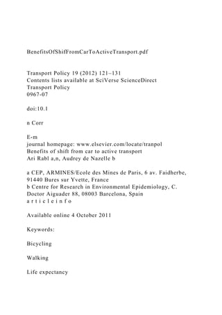
![Mortality
Air pollution
Accidents
0X/$ - see front matter & 2011 Elsevier Ltd. A
016/j.tranpol.2011.09.008
esponding author.
ail address: [email protected] (A. Rabl).
a b s t r a c t
There is a growing awareness that significant benefits for our
health and environment could be
achieved by reducing our use of cars and shifting instead to
active transport, i.e. walking and bicycling.
The present article presents an estimate of the health impacts
due to a shift from car to bicycling or
walking, by evaluating four effects: the change in exposure to
ambient air pollution for the individuals
who change their transportation mode, their health benefit, the
health benefit for the general
population due to reduced pollution and the risk of accidents.
We consider only mortality in detail,
but at the end of the paper we also cite costs for other impacts,
especially noise and congestion. For the
dispersion of air pollution from cars we use results of the](data:image/gif;base64,R0lGODlhAQABAIAAAAAAAP///yH5BAEAAAAALAAAAAABAAEAAAIBRAA7)