This presentation was presented by Florian Wellmann, Mark Lindsay and Mark Jessell and the recent EGU 2015 conference. ____ Geological models are widely used to represent the structural setting of the subsurface. Commonly, a single model is generated for a region, representing the best interpretation of the structural setting in the light of all available information. It is, however, widely accepted that a such created model still contains uncertainties. We hypothesise here that it is possible to transform a single kinematic model into a powerful predictive tool for scenario analysis and uncertainty quantification. We extend the functionality of a kinematic structural and geophysical modelling approach, implemented in the software Noddy, with a set newly developed Python modules to expose, generalise and automate essential parts of the modelling workflow. We show how these methods enable us to quickly generate and analyse different geological scenarios. In addition to the geological model, Noddy also enables the direct calculation of geophysical fields of gravity and magnetics. We can use this functionality to compare the model to measured potential fields. With an example for a fold and thrust belt model, we show how to quickly estimate how changes in the model (due to parameter uncertainties, for example) affect the calculated gravity field in the model range. Finally, we present the possibility to efficiently generate an ensemble of model realisations for predictive geomodel analysis with an application to a case study in the Gippsland Basin, Victoria. The results show that our approach can successfully extend the functionality of traditional modelling methods with an additional layer of predictive power towards an efficient evaluation of uncertainties in structural geological models.

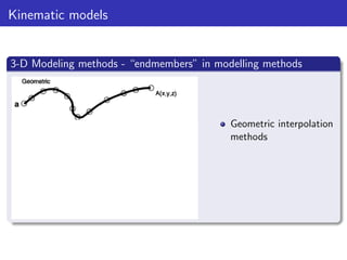
1. Kinematic models
3-D Modeling methods - “endmembers” in modelling methods
Geometric interpolation
methods

2. Kinematic models
3-D Modeling methods - “endmembers” in modelling methods
Geometric interpolation
methods
Full dynamic simulations

3. Kinematic models
3-D Modeling methods - “endmembers” in modelling methods
Geometric interpolation
methods
Kinematic modelling
approach
Full dynamic simulations

4. Simple fault model
(d) Event 1 + Event 2: combined effect of faults
(a) Initial Stratigraphy
(c) Event 2: Fault E(b) Event 1: Fault W
Example of a fault model:
initial stratigraphic
pile,

5. Simple fault model
(d) Event 1 + Event 2: combined effect of faults
(a) Initial Stratigraphy
(c) Event 2: Fault E(b) Event 1: Fault W
Example of a fault model:
initial stratigraphic
pile,
effect of the first
fault only,

6. Simple fault model
(d) Event 1 + Event 2: combined effect of faults
(a) Initial Stratigraphy
(c) Event 2: Fault E(b) Event 1: Fault W
Example of a fault model:
initial stratigraphic
pile,
effect of the first
fault only,
effect of the second
fault only,

7. Simple fault model
(d) Event 1 + Event 2: combined effect of faults
(a) Initial Stratigraphy
(c) Event 2: Fault E(b) Event 1: Fault W
Example of a fault model:
initial stratigraphic
pile,
effect of the first
fault only,
effect of the second
fault only,
combined effect of
both faults.

8. Code example for fault model

9. Kinematic modelling
Advantage
Parameterisation of geological history
High level of complexity possible with multiple events
Automation and implementation in Python scripts straight-forward
Very fast computation, even for complex models

10. Kinematic modelling
Advantage
Parameterisation of geological history
High level of complexity possible with multiple events
Automation and implementation in Python scripts straight-forward
Very fast computation, even for complex models
More examples

11. Scenario Testing and Sensitivity Analysis for
3-D Kinematic Models and Geophysical Fields
J. Florian Wellmann1, Mark Lindsay2 and Mark Jessell2
(1) Graduate School AICES, RWTH Aachen University
(2) Centre for Exploration Targeting (CET), The University of Western Australia
PICO presentation — EGU 2015
April 15, 2015

12. Overview of Presentation
“PICO madness”
Fault exampleBasic concept Geophysics
Automation and
set-up of repro-
ducible experiments

13. Back to overview .
Kinematic modelling concept
Idea behind kinematic modelling
Evaluate interaction between tectonic events in geological history

14. Back to overview .
Kinematic modelling concept
Idea behind kinematic modelling
Evaluate interaction between tectonic events in geological history
Define influence of events on pre-existing geology with purely
kinematic methods

15. Back to overview .
Kinematic models
3-D Modeling methods - “endmembers” in modelling methods
Geometric interpolation
methods

16. Back to overview .
Kinematic models
3-D Modeling methods - “endmembers” in modelling methods
Geometric interpolation
methods
Full dynamic simulations

17. Back to overview .
Kinematic models
3-D Modeling methods - “endmembers” in modelling methods
Geometric interpolation
methods
Kinematic modelling
approach
Full dynamic simulations

18. Back to overview .
Additional considerations
Advantage
Parameterisation of geological history
High level of complexity possible with multiple events
Very fast computation, even for complex models
Direct extension to geophysical forward modelling

19. Back to overview .
Additional considerations
Advantage
Parameterisation of geological history
High level of complexity possible with multiple events
Very fast computation, even for complex models
Direct extension to geophysical forward modelling
Disadvantage
Simplification of processes (no dynamics!)

20. Back to overview .
Additional considerations
Advantage
Parameterisation of geological history
High level of complexity possible with multiple events
Very fast computation, even for complex models
Direct extension to geophysical forward modelling
Disadvantage
Simplification of processes (no dynamics!)
Implementation
Original code in C (first published in 70’s!)
pynoddy: new implementation in Python, linking to C-code
(Now) a high level of flexibility for automation
All open source: see pynoddy project page.

21. Back to overview .
Setting up a simple model with pynoddy
Model set-up
A simple pynoddy model can be defined with a few lines of code. The first
step is (usually) to define an initial stratigraphy, for example as a
sedimentary layer-cake:

22. Back to overview .
Simple fault model
(d) Event 1 + Event 2: combined effect of faults
(a) Initial Stratigraphy
(c) Event 2: Fault E(b) Event 1: Fault W Development of a fault
network model with
pynoddy:
initial stratigraphic
pile,

23. Back to overview .
Setting up a simple model with pynoddy
Adding one fault
Additional code to add both faults:

24. Back to overview .
Simple fault model
(d) Event 1 + Event 2: combined effect of faults
(a) Initial Stratigraphy
(c) Event 2: Fault E(b) Event 1: Fault W
Development of a fault
network model with
pynoddy:
initial stratigraphic
pile,

25. Back to overview .
Simple fault model
(d) Event 1 + Event 2: combined effect of faults
(a) Initial Stratigraphy
(c) Event 2: Fault E(b) Event 1: Fault W
Development of a fault
network model with
pynoddy:
initial stratigraphic
pile,
effect of the first
fault only,

26. Back to overview .
Simple fault model
(d) Event 1 + Event 2: combined effect of faults
(a) Initial Stratigraphy
(c) Event 2: Fault E(b) Event 1: Fault W
Development of a fault
network model with
pynoddy:
initial stratigraphic
pile,
effect of the first
fault only,
effect of the second
fault only,

27. Back to overview .
Simple fault model
(d) Event 1 + Event 2: combined effect of faults
(a) Initial Stratigraphy
(c) Event 2: Fault E(b) Event 1: Fault W
Development of a fault
network model with
pynoddy:
initial stratigraphic
pile,
effect of the first
fault only,
effect of the second
fault only,
combined effect of
both faults.

28. Back to overview .
Changing aspects of existing models
Concept
Basic concept: possible to load and modify
existing history files, e.g.:
Created with (original) Noddy GUI
(limited to Windows);
From online repository, Atlas of
Structural Geophysics
Loading models from the Atlas of Virtual Geophysics
It is possible to directly load models into the Python modules:

29. Back to overview .
Selected model from Virtual Geophysics Atlas
Figure: Sections through the fold and thurst belt model in (a) NS-direction, and
(b) EW-direction (vertical exaggeration of 1.5) through the centre of the model.
(c) Three-dimensional representation for the central three layers of the fold and
thrust belt model. The gray surfaces correspond to the location of the sections in
the figure above.

30. Back to overview .
Calculation of geophysical fields
Gravity and Magnetic field calculation
pynoddy enables the calculation of geophysical fields directly from
the generated block models.
In the combination with the Python scripts, it is easily possible to
change aspects of model and evaluate the effect on the simulated
potential field.
Example of gravity calculation
Change event parameters:
Update modelled gravity field:

31. Back to overview .
Comparison of gravity fields
Figure: Gravity of original and changed model

32. Back to overview .
Stratigraphic difference between generated block models
Figure: Stratigraphic difference between the two generated block models

33. Back to overview .
Automation and reproducible experiments
Concept
Main idea: enable definition of reproducible experiments
Implementation
Definition of an Experiment class to combine pre- and
postprocessing methods
Additional basic settings to store experiment settings (number of
realsiations, random seeds, etc.)
Specific experiment types can easily be defined by inheriting from the
base experiment class.

34. Back to overview .
Experiment setup
Creating an experiment object
Experiment objects can be created directly from an existing history file:
Experiment classes combine pre- and postprocessing of kinematic models
and the model is recomputed whenever required:
Which directly creates this section plot:

35. Back to overview .
Outlook
IPython Notebooks
Many more examples about model manipulation and experiment extension
are available online as interactive IPython notebooks!

36. Back to overview .
Gippsland Basin study
Experiment for uncertainty analysis in the Gippsland Basin

37. Back to overview .
More information
Thank you for viewing the presentation!
More information
If you are interested, please have a look at available online resources:
pynoddy repository on github (feel free to download, modify, and
contribute!)
Online documentation about pynoddy
There is also a set of online tutorials available.
See Abstract for this presentation