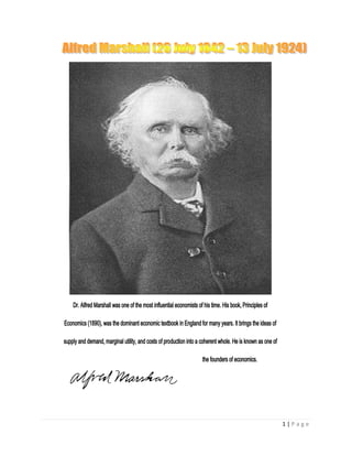
1. Dr. Alfred Marshall was one of the most influential economists of his time. His book, Principles of
Economics (1890), was the dominant economic textbook in England for many years. It brings the ideas of
supply and demand, marginal utility, and costs of production into a coherent whole. He is known as one of
the founders of economics.
1|Page
2. Consumer’s Surplus
•Marshall interpreted a demand curve as a willingness to pay at
the margin curve
•Consumer is willing to pay more for the first few units of a
good than for subsequent units
•If the consumer pays a single price for all units bought then the
total willingness to pay for those units will exceed the amount
actually paid
•This is consumer’s surplus
2|Page
3. Demand Theory
•The demand curve is interpreted as a schedule of
―Demand Prices‖
•What is held constant along this demand curve?
•Marshall assumes both constant money income and
constant real income (constant MU of income)
•This rules out any significant income effects
•Marshall’s ―Law of Demand
3|Page
4. Marshall on Production
•Factors of production: land, labour, capital, and organization
•Diminishing returns in agriculture
•Diminishing returns can also occur with fixed factors other than land
•Increasing returns in industry with concentration of industry in
particular localities
•Increased productivity in industry due to larger scale of particular
firms--increased specialization of labour and machinery
•Economies of buying and selling on a large scale
•Forms of business organization and the problems of maintaining energy
and efficiency
•Joint stock companies and problems of agency
•Distinction between external and internal economies
–External economies are economies derived from the general
development of an industry (external to individual firms)
–Internal economies derived from the size of individual firms
(internal to the firm)
•Tendency to decreasing returns in agriculture and natural resource
industries
•Tendency to increasing returns in other industries
–An increase of labour and capital leads generally to improved
organization which increases the efficiency of labour and capital
•But limits to the size of particular firms
•Biological analogy and the life cycle of firms
•Concept of the representative firm--firm with average access to internal
and external economies
4|Page
6. Long Run Supply
•In industries where external economies dominate, growth in industry size will
lower the costs of all firms
•Long run industry supply curve will be downward sloping (decreasing cost
industry)
•If external diseconomies dominate industry growth raises costs for all firms
•Long run industry supply curve will be upward sloping (increasingcost industry)
•If external economies and diseconomies just cancel each other out then the costs
of firms will not be affected by industry growth
•Long run supply curve will be horizontal (constant cost industry)
•Marshall though most industries other than natural resource industries had
declining long run costs
•What might these external economies consist of? •Reduction in factor cost due to
industry growth creating a pool of trained labour in that locality
6|Page
8. Marshall is considered to be one of the most influential economists of
his time, largely shaping mainstream economic thought for the next
fifty years, and being one of the founders of the school of neoclassical
economics. Although his economics was advertised as extensions and
refinements of the work of Adam Smith, David Ricardo, Thomas Robert
Malthus and John Stuart Mill, he extended economics away from its
classical focus on the market economy and instead popularized it as a
study of human behavior. He downplayed the contributions of certain
other economists to his work, such as Leon Walras, Vilfredo Pareto and
Jules Dupuit, and only grudgingly acknowledged the influence of
Stanley Jevons himself.
Marshall's influence on codifying economic thought is difficult to deny.
He popularized the use of supply and demand functions as tools of
price determination (previously discovered independently by Cournot);
modern economists owe the linkage between price shifts and curve
shifts to Marshall. Marshall was an important part of the "marginalist
revolution;" the idea that consumers attempt to adjust consumption
until marginal utility equals the price was another of his contributions.
The price elasticity of demand was presented by Marshall as an
extension of these ideas. Economic welfare, divided into producer
surplus and consumer surplus, was contributed by Marshall, and
indeed, the two are sometimes described eponymously as 'Marshallian
surplus.' He used this idea of surplus to rigorously analyze the effect of
taxes and price shifts on market welfare.
8|Page
9. He demonstrated the tremendous theoretical power of demand and supply
curves, and bequeathed to economics the critical distinction between the short
run and the long run.
9|Page
10. Milton Friedman (July 31, 1912 – November 16, 2006)
Friedman was a Marshallian,but he was a macroeconomist. He had his own researchAgenda:
Money and Inflation.And he was out to counter Keynesian theory and policy.
Milton Friedman was an American economist, statistician, and author who taught at the
University of Chicago for more than three decades. He was a recipient of the Nobel Memorial
Prize in Economic Sciences, and is known for his research on consumption analysis,
monetary history and theory, and the complexity of stabilization policy.[1] As a leader of the
Chicago school of economics, he influenced the research agenda of the economics
profession.
10 | P a g e
11. MV = PQ
M is the money supply
(outside the banking system).
V is money’s velocity of circulation.
P is the price level.
Q is the economy’s output.
PQ is total expenditures (E).
MV is total income (Y)
MV = PQ This is the “Equation of Exchange.” No economist, dead or living,
has ever denied that MV actually does equal PQ... …because V is defined as
PQ/M.
MV = PQ
In normal times:
V doesn’t change much.
Q changes in the low single digits.
Keynes believed that the velocity of money was subject to dramatic and
unpredictable change. He believed that people “hoard” money, more so
some times than others. (increased hoarding means a decrease in velocity.)
In extreme episodes, people may be overcome by the “fetish of liquidity,”
the fetish often accompanying the waning of animal spirits.
11 | P a g e
12. MV = PQ In the long run and with a constant V, the price level (P) moves in
proportion to the money supply (M) in a no-growth (i.e., constant-Q)
economy. This is “The Quantity Theory of Money.” A more descriptive name
would be: “The Quantity of Money Theory of the Price Level.”
MV = PQ
More generally,
In the long run, money-supply growth in excess of real economic growth
impinges wholly on the price level (P) and not at all on the level of real
output.
Put bluntly: you can’t create real wealth by slapping green ink on paper.
12 | P a g e
13. Monetarism
Some diagnostics: With the “Monetarist Rule” in effect (2 or 3%) and a
constant V, the rate of inflation would be zero—or very close to zero. Has
the rate of inflation been zero?
Some diagnostics:
CPI for 1982-1984 = 100 CPI for January 2010 = 216 That is, prices on
average are more than double now what they were in the early 1980s.
13 | P a g e
14. Some diagnostics:
Has Q been falling for the past 25 years? Has V been rising for the past 25
years? Has M been rising for the past 25 years?
Do labor unions cause inflation?
No. But they can cause the prices of goods made by unionized labor to rise
and the prices of goods made by non-unionized labor to fall.
However, if the central bank increases the money supply in an attempt to
neutralize the effects of labor unions, the general price level will rise.
14 | P a g e
16. JOHN MAYNARD KEYNES,(5 JUNE 1883–21 APRIL 1946)
J.M. Keynes was a British economist whose ideas have profoundly
affected the theory and practice of modern macroeconomics, as well as
the economic policies of governments. He greatly refined earlier work
on the causes of business cycles, and advocated the use of fiscal and
monetary measures to mitigate the adverse effects of economic
recessions and depressions. Keynes is widely considered to be one of
the founders of modern macroeconomics, and to be the most
influential economist of the 20th century.
16 | P a g e
17. THE INFLUENCE OF THE GENERAL THEORY
To return to the General Theory: its influence on both economic thinking and economic
practice was profound. The “Keynesian revolution” was far more than a figure of speech.
From shortly after the publication of the book in 1936 to at least the 1960s, the majority of
professional economists, and certainly the most prominent, termed themselves
“Keynesians.” Those who called themselves non- or anti-Keynesians were a beleaguered
minority, supplemented, it must be said, by some important writers on economics who were
not members of the professional guild.
The interest rate, in turn, he regarded as determined by “liquidity preference,”
the third of his key concepts. “An individual’s liquidity-preference
is given by a schedule of the amounts of his resources, valued in terms of
money or of wage-units, which he will wish to retain in the form of money
in different sets of circumstances.” He regarded the amount of their assets that
individuals would want to hold in the form of money as depending on both
income and the interest rate—income because that would affect the amount
held for “transactions- and precautionary-motives,” the interest rate, because
that would affect the amount held “to satisfy the speculative-motive.”
If, as Keynes did, we let Y be income, identical with the value of output,
C be consumption, I be investment, L liquidity preference, M the quantity of
Money, and r the interest rate, then aggregate demand is given by
Y = C(Y) + I(r),(1)
and the demand for money by
M = L(Y, r). (2)
In line with his implicit assumption about the relative speed of adjustment
of prices and output, Keynes regarded supply as essentially passive, expanding
or contracting as demand expanded or contracted, subject only to the proviso
that employment is less than “full,” which he defined as the point at which an
increase in aggregate demand would call forth no additional workers willing to
work at the wage offered. This leads him to regard aggregate supply as given
simply by aggregate demand, or
YS = YD, (3)
and the level of aggregate supply and demand as affecting not a price but solely
employment.
17 | P a g e
18. If we regard the interest rate as fixed, along with other prices, then equations
(1) and (3) define the famous Keynesian “multiplier” (attributed by Keynes to
Richard Kahn). For a simple version, assume that the consumption function is
linear:
C = a + bY, (4)
withb, of course, less than one. Substituting (4) in (1) and solving for Y, we
have
Y=
a + I (r )
1−b
=µ1
1 − b¶[a + I(r)]. (5)
The multiplier is 1/(1 − b), which, given that b is between zero and unity,
is necessarily greater than unity. The multiplicand, (a + I), came to be termed
“autonomous” spending, i.e., spending not dependent on the level of income. In
addition, once government was introduced into the analysis, autonomous spending
was regarded as including not only autonomous consumption spending (a)
and investment (I ) but also government spending.
Equations (1) and (3) define also the equally famous “Keynesian cross,”
18 | P a g e
19. Marvelously simple. A key that apparently unlocks the mystery of
Long-continued unemployment: inadequate autonomous spending or too low a
Propensity to consume. Increase either, or both, being careful simply not to go
Too far, and full employment could be attained. What a wonderful prescription:
for consumers, spend more out of your income, and your income will rise;
for governments, spend more, and aggregate income will rise by a multiple of
your additional spending; tax less, and consumers will spend more with the
same result. Though Keynes himself, and even more, his disciples, produced
Much more sophisticated and subtle versions of the theory, this simple version
Contains the essence of its great appeal to non-economists and especially governments.
Here was one of the most famous and respected economists in the
World informing governments that the way to full employment was paved with
19 | P a g e
20. higher spending and lower taxes.
Of course, Keynes recognized that changes in prices, interest rates, and
quantity of money did have effects that provided alternative avenues of escape
from the so-called “underemployment equilibrium.” At best, it was a transitory
equilibrium position, the existence of which would set in motion self-corrective
forces. But Keynes tended to rule out these alternative avenues of escape as of
no practical significance because of his empirical judgment that prices, wages,
and interest rates were highly sluggish. Indeed, some commentators on Keynes
maintain that he deliberately overstated his case in order to shock the economics
profession into paying attention—a tactic that is common to every innovator,
whether it be of an idea or a product.
Only one alternative avenue of adjustment is explicitly present in equations
(1) and (2)—via the interest rate and the quantity of money. This avenue,
analyzed at some length in the General Theory, and found wanting to produce,
by itself, a full employment equilibrium, also was rapidly incorporated in an
alternative, more sophisticated graphical representation of the Keynesian system
developed almost simultaneously by John Hicks and Roy Harrod.11 Figure
2 presents Hicks’s IS-LM version, which very quickly became the orthodox
version.
In this diagram, the vertical axis is the interest rate. The horizontal axis is
income expressed in wage-units, so that it is also output and employment. The
IS curve traces equation (5), i.e., it shows the combinations of interest rate and
output that would satisfy equation (1): the higher the interest rate, the lower
investment and hence income, and conversely, which is why the IS curve has
a negative slope. Put differently, it shows the combinations of interest rate and
output at which the amount some people wish to invest is equal to the amount
other people wish to save, which is what explains the S in IS. But note that the
accommodation of saving to investment is produced not by the direct effect of
the interest rate on saving, but by the effect of the level of income on saving,
via the propensity to consume.
The LM curve traces equation (2) for a fixed quantity of money.
20 | P a g e
21. The intersection of the IS and LM curve at YO is the counterpart of the
intersection of the aggregate demand and supply curves in Figure 1 at YO. Similarly,
the IS0 curve is the counterpart of the Y0O curve in Figure 1, reflecting a
higher level of investment. It is the IS curve moved to the right by the change
in income assumed to be produced by the increase in investment—the change
in investment times the investment multiplier.
What is new in Figure 2 are the LM curves. Each LM curve is for a specific
quantity of money: the LM curve for M = MO, the (LM)0 curve for M = M0O,
which is larger than MO. For the community to hold the larger quantity of
money willingly, either the interest rate must be lower for a given income or
income higher for a given interest rate, which is why the (LM)0 curve is to the
right of the LM curve.
The IS curve in the diagram embodies a possible Keynesian escape from
underemployment via increases in investment (or, more generally, autonomous
spending including government spending). Let autonomous spending be high
21 | P a g e
22. enough so that the IS curve intersects the LM curve at point F, and full employment
would be attained with the initial quantity of money.
Figure 3 shows an extreme version of these assumptions: perfectly inelastic
investment and perfectly elastic liquidity preference.We are back to the Keynesian
cross of Figure 1. No changes in the quantity of money can produce a full
employment equilibrium. This LM curve depicts a “liquidity trap,” of which
Keynes wrote, “whilst the limiting case might become practically important in
future, I know of no example of it hitherto.
22 | P a g e