

Recomendados
Mais conteúdo relacionado
Mais procurados
Mais procurados (20)
Semelhante a Statistics for management
Semelhante a Statistics for management (20)
Último
Último (20)
Statistics for management
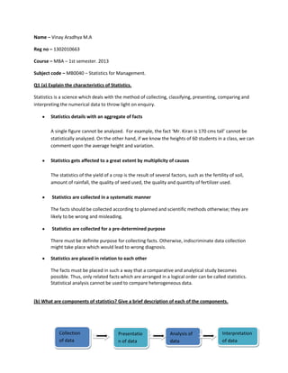
- 1. Name – Vinay Aradhya M.A Reg no – 1302010663 Course – MBA – 1st semester. 2013 Subject code – MB0040 – Statistics for Management. Q1 (a) Explain the characteristics of Statistics. Statistics is a science which deals with the method of collecting, classifying, presenting, comparing and interpreting the numerical data to throw light on enquiry. Statistics details with an aggregate of facts A single figure cannot be analyzed. For example, the fact ‘Mr. Kiran is 170 cms tall’ cannot be statistically analyzed. On the other hand, if we know the heights of 60 students in a class, we can comment upon the average height and variation. Statistics gets affected to a great extent by multiplicity of causes The statistics of the yield of a crop is the result of several factors, such as the fertility of soil, amount of rainfall, the quality of seed used, the quality and quantity of fertilizer used. Statistics are collected in a systematic manner The facts should be collected according to planned and scientific methods otherwise; they are likely to be wrong and misleading. Statistics are collected for a pre-determined purpose There must be definite purpose for collecting facts. Otherwise, indiscriminate data collection might take place which would lead to wrong diagnosis. Statistics are placed in relation to each other The facts must be placed in such a way that a comparative and analytical study becomes possible. Thus, only related facts which are arranged in a logical order can be called statistics. Statistical analysis cannot be used to compare heterogeneous data. (b) What are components of statistics? Give a brief description of each of the components. Collection of data Presentatio n of data Analysis of data Interpretation of data
- 2. Basis components of Statistics According to Croxton and Cowden Collection of data : Careful planning is required while collecting data. Two methods used for collecting data are census method and sampling method. The investigator has to take care while selecting an appropriate collection method. Presentation of data : The collection data is usually presented for further analysis in a tabular, diagrammatic or graphic from and it is condensed, summarized and visually represented in a tabular or graphical form. Tabulation is a systematic arrangement of classified data in rows and columns. For the representation of data in diagrams, we use different types of diagrams such as one-dimensional, two-dimensional and three dimensional diagrams. Analysis of data The data presented has to be carefully analyzed to make any inference from it. The inference can be various types, for example, as measure of central tendency, desperation, correlation or regression. Interpretation of data The final step is to draw conclusions from the analyzed data. Interpretation requires high degree of skill and experience. We can interpret the data easily from pie-charts. Q2. Explain the objectives of statistical average. What are the requisites of a good average? The statistical average or simply an average refers to the measure of middle value of the data set. The objectives of statistical average are to: Present mass data in a concise form: The mass data is condensed to make the data readable and to use it for further analysis. It is very difficult for human mind to grasp a large body of numerical figures. A measure of average is used to summarize such data into a single figure, which makes it easier to understand. Facilities comparison: It is difficult to compare two different sets of mass data. However, we can compare those two after computing the averages of individual data sets. While comparing the same measure of average should be used. It leads to incorrect conclusions when the mean salary of employees is compared with the median salary of the employees.
- 3. Establish relationship between data sets: The average can be used to draw inferences about the unknown relationships between the data sets. Computing the averages of the data sets is helpful for establishing the average of population. Provide basis for decision making: In many fields such as business, finance, insurance and other sectors, managers compute the averages and draw useful inferences or conclusions for taking effective decisions. Requisites of a good average The following are the requisites of a good average: It should be simple to calculate and easy to understand. It should be based on all the values. It should not be affected by extreme values. It should not be affected by sampling fluctuation. It should be rigidly defined, preferably by an algebraic formula, so that different persons obtain the same value for a given set of data. Should be suitable for further mathematical treatment. Vigorously defined Capable of simple interpretation Capable of mathematical manipulation. Not unduly influenced by one or two extremely large or small values. Dependent on all the observed values. Q3. Mention the characteristics of a Chi-square test. The Chi-square test is one of the most commonly used non-parametric tests in statistical work. The following are the characteristics of Chi-Square test ( 2 test). The 2 test is based on frequencies and not on parameters It is a non-parametric test where no parameters regarding the rigidity of population of populations are required Additive property is also found in 2 test The 2 test is useful to test the hypothesis about the independence of attributes The 2 test can be used in complex contingency tables The 2 test is very widely used for research purposes in behavioral and social sciences including business research It is defined as: Where, ‘O’ is the observed frequency and ‘E’ is the expected frequency.
- 4. b. Answer: Let us take the hypothesis that the sampling techniques adopted by research workers are similar (i.e., there is no difference between the techniques adopted by research workers). This being so, the expectation of a investigator classifying the people in i. Poor income group = (200 * 300) / 500 = 120 ii. Middle income group = (200 * 150) / 500 = 60 iii. Rich income group = (200 * 50) / 500 = 20 Similarly the expectation of B investigator classifying the people in i. Poor income group = (300 * 300) / 500 = 180 ii. Middle income group = (300 * 150) / 500 = 90 iii. Rich income group = (300 * 50) / 500 = 30 We can now calculate as follows: Groups Observed frequency Oij Expected frequency Eij Oij– Eij (Oij– Eij)2 Eij Investigator A classifies people as poor 160 120 40 1600/120 = 13.33 classifies people as middle class people 30 60 -30 900/60 = 15.00 classifies people as rich 10 20 -10 100/20 = 5.00 Investigator B classifies people as poor 140 180 -40 1600/180 = 8.88 classifies people as middle class people 120 90 30 900/90 = 10.00 classifies people as rich 40 30 10 100/30 = 3.33 Hence, χ 2 =∑{ (O ij – Eij) 2 /Eij} = 55.54 Degrees of freedom = (c – 1) (r – 1) = (3 – 1) (2 – 1) = 2. The table value of χ for two degrees of freedom at 5 per cent level of significance is 5.991. The calculated value of χ is much higher than this table value which means that the calculated 2value cannot be said to have arisen just because of chance. It is significant. Hence, the hypothesis does not
- 5. hold good. This means that the sampling techniques adopted by two investigators differ and are not similar. Naturally, then the technique of one must be superior to that of the other Q4. What do you mean by cost of living index? Discuss the methods of construction of cost of living index with an example for each. The ‘Cost of living index’, also known as ‘consumer price index’ or ‘cost of living price index’ is the country’s principal measure of price change. The consumer price index helps us in determining the effect of rise and fall in prices on different classes of consumers living in different areas. The cost of living index does not measure the actual cost of living or the fluctuations in the cost of living due to causes other than the change in price level. However, its object is to find out how much the consumers of a particular class have to pay for a certain quantity of goods and services. (i). Utility of consumer price index numbers It is useful to measure the change in purchasing power of currency, real income. It helps the government in formulating wage policy, price policy, taxation and general economic policies. (ii). Assumptions of cost of living Index Numbers Cost of living index number is based on the following assumptions. Similar needs The needs of the people for which this index number is constructed are same. Same goods Cost of living index numbers are true on the average. (iii). Steps in construction of cost of living index numbers There are 5 steps involved in construction of cost of living index numbers. Step 1: Select the class of people Step 2: Define scope of the index Step 3: Conduct family budget inquiry Step 4: Obtain price quotations Step 5: Prepare a frame or list of persons Method of constructing consumer price index: There are two methods for constructing consumer price index number. They are: I. Aggregate expenditure method II. Family budget method or method of weighted average of price relatives. Aggregate expenditure method
- 6. This is based on Laspeyre’s method where the base year quantities are taken as weights (W = Qo). ∑ P1 Q0 Po1 = -------------------- x 100 ∑ P0 Q0 Family budget method Family budget method or the method of weighted relatives is the method where weights relatives is the method where weight are the value (Po Qo) in the base year often denoted by W. ∑ PW P1 Po1 = --------------------, where P= ------- X 100 for each item and ∑ W P0 W = value weight, i.e. PoQo Example Calculate the cost of living index for the current year on the basis of the base year from the following data, using Solution: - Aggregate expenditure Method The formula of aggregate expenditure method is giving by:
- 7. ∑ P1 Q0 315.6 Po1 = -------------------- x 100 = -------------- x 100 = 106.87 ∑ P0 Q0 295.3 Therefore the cost of living index number is 106.87 Q5. Define trend. Enumerate the methods of determining trend in time series. The trend is a pattern of data. The trend shows how the series has been moving in the past and what its future course is likely to be over a long period of time. To measure the secular trend, the short-term variations should be removed and irregularities should be smoothed out. The following are the methods of measuring trend. Graphic method The values of the time series are plotted on a graph paper with the time (t) along x-axis and the values of the variable (y) along y-axis. A freehand curve is drawn through these points in such a manner that it may show a general trend. A free hand curve removes the short-term variations and irregular movements. It is the simplest method, Time and labor is saved. It is very flexible method as it represents both linear and non-linear trends. The main drawback of this method is that it is highly subjective as different persons will draw different free hand curves. Because of its subjective nature it is useless in forecasting. Semi-Average Method This method is sometimes used when a straight line appears to be an adequate expression of trend. In this method, the original data are divided into two equal parts. The averages of each part are then calculated. The average of each part is centered in the period of the time of the part from which it has been computed and then plotted on the graph paper. In this way, a line may be drawn to pass through the plotted points which give the trend line. In case of odd number of years, the mid-year is eliminated while dividing the data into two equal parts. This method is not subjective and ·everyone gets the same trend line. It is possible to extend the trend line both the ways to estimate future or past values. But the method assumes the presence of linear trend which may not exist. Moving Average Method Moving averages method is used for smoothing the time series. It smoothens the fluctuations of the data by the moving averages method. Least squares method
- 8. The method of least squares is a standard approach to the approximate solution of over determined systems, i.e., sets of equations in which there are more equations than unknowns. "Least squares" means that the overall solution minimizes the sum of the squares of the errors made in the results of every single equation. Q6. The following data represent the number of units of production per day turned out by 5 different workmen using different types of machines. Workmen Machine type A B C D 1 44 38 47 36 2 46 40 52 43 3 34 36 44 32 4 43 38 46 33 5 38 42 49 39 i) Test whether the mean productivity is the same for the four different machine types. ii) Test whether 5 men differ with respect to mean productivity. Let H0: (a) Mean Productivity is same for all machines (b) Men do not differ with respect to mean productivity decoding the data by subtracting 40 from each figure. Source of Variation Sum of Squares Degrees of Freedom Mean Square Variance Ratio Between machine type 338.8 3 112.933 F1 = 112.933 / 6.142 = 18.387 Between workers 161.5 4 40.375 F2 = 40.375 / 6.574 = 6.574 Residual error 73.7 12 6.142 Total 574 19 (a) F0.05 = 3.49 at df1 = 3 and df2 = 12. Since the calculated value F1 = 18.387 is greater than the table value, the null hypothesis is rejected. (b) F0.05 = = 3.26 at df1 = 4 and df2 = 12. Since the calculated value F2 = 6.574 is greater than the table value, the null hypothesis is rejected.