If you are looking for help with conditional formatting in Excel then download our Free Guide to Microsoft Excel -Conditional formatting

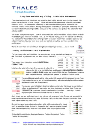
1. If only there was better way of doing…. CONDITIONAL FORMATTING
Your boss has just come over to tell you he/she is really happy with the report you’ve created, then
comes the request for a “small change”…’could you add some colour to the information to make it
stand out more? The people I am presenting to like to have something visual rather than just
numbers…thanks’. Panic sets in…having already spent several hours getting the data ready you are
now confronted with colouring in all the cells just so that someone can ‘picture’ the data rather than
actually read it!
And so the slow process begins…click on a cell, check the value, then select a colour based on a set
of conditions your boss has invented. Then…to add insult to injury, just as you are half way through,
you are told that the conditions have ‘changed a bit’ because it meant there would be too many red
cells on the sheet. You now have to go back and recheck everything and hope you don’t miss
anything out.
We’ve all been there and spent hours doing this most boring of chores……but no need!
Thankfully, Excel has CONDITIONAL FORMATTING.
You can create rules and conditions that automatically format your cells any way you
like. First of all, highlight the cells you want to apply the rule(s)
to.
Then, select from the options under CONDITIONAL
FORMATTING.
Let’s take the table to the right. If we wanted all cells with a
value under 500 to be highlighted we would select HIGHLIGHT CELLS RULES,
click on the LESS THAN option and type in 500 in the box. Finally select how you
want the cell to appear. Use any of the presets ,or go for full custom format.
You should see any cells with a value under 500 appear with the selected format. Now,
if you make changes to any of the cell values they will automatically format themselves.
No need to check and no extra work!
You can set rules to highlight data that is between/ greater than/equal to user defined
values as well as identify text, dates and even duplicated or unique data! There are
TOP/BOTTOM type rules, custom rules based on formulas……basically if it needs
highlighting for some reason there is a way of setting it up.
Don’t forget, you are not limited to only one rule per cell or range of cells. Once a rule is crated it is
easy to edit to suit any demanding boss. And to top it all, you also have the option to display data
bars, colour scales and even icons!
So next time your boss asks you to make a table a bit more colourful or visual
you’ll be spoilt for choice. And as for those who don’t seem to be able to read
data, they can have pretty flags and traffic lights. What more could you ask
for?
Written by Richard Harker, Business Systems Training Consultant, Thales
Training & Consultancy
Contact us: thales-trainingconsultancy.com twitter.com/thalestraining
0800 163 469 http://blog.thales-trainingconsultancy.com