First post of a Data Science blog about Linear Regression using Matlab. For more information, please visit: http://datascienceinsights.blogspot.com.br/ https://github.com/tadeuferreirajr/MachineLearning

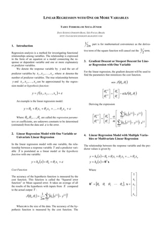
1. LINEAR REGRESSION WITH ONE OR MORE VARIABLES
TADEU FERREIRA DE SOUSA JÚNIOR
DATA SCIENCE INSIGHTS BLOG, SÃO PAULO, BRAZIL
HTTP://DATASCIENCEINSIGHTS.BLOGSPOT.COM
1. Introduction
Regression analysis is a method for investigating functional
relationships among variables. The relationship is expressed
in the form of an equation or a model connecting the re-
sponse or dependent variable and one or more explanatory
or predictor variables.
We denote the response variable by y and the set of
predictor variables by nxxx ,,, 21  , where n denotes the
number of predictor variables. The true relationship between
y and nxxx ,,, 21  can be approximated by the regres-
sion model or hypothesis function:
   nxxxfy ,,, 21 
An example is the linear regression model:
  nn xxxy 22110
Where n ,,, 10  are called the regression parame-
ters or coefficients, are unknown constants to be determined
(estimated) from the data and  is the error.
2. Linear Regression Model with One Variable or
Univariate Linear Regression
In the linear regression model with one variable, the rela-
tionship between a response variable Y and a predictor vari-
able X is postulated as a linear model or the hypothesis
function with one variable:
    110 xxhy
Cost Function
The accuracy of the hypothesis function is measured by the
cost function. This function is called the “Squared error
function” or Mean squared error. It takes an average of all
the results of the hypothesis with inputs from X compared
to the actual output Y :
   
   
 

m
i
ii
yxh
m
J
1
2
10
2
1
, 
Where mis the size of the data. The accuracy of the hy-
pothesis function is measured by the cost function. The
m2
1 part is for mathematical convenience as the deriva-
tive term of the square function will cancel out the
2
1 term.
3. Gradient Descent or Steepest Descent for Line-
ar Regression with One Variable
For the linear regression, the gradient descent will be used to
find the parameters that minimizes the cost function.
min  10 ,J
 10
1
0
1
1
1
0
,




Ji
i
i
i














Deriving the expression
 
   
 
 
   
   
































m
i
iii
m
i
ii
i
i
i
i
xyxh
yxh
m
1
1
1
0
1
1
1
0







4. Linear Regression Model with Multiple Varia-
bles or Multivariate Linear Regression
The relationship between the response variable and the pre-
dictor values is given by
 
  xθT
nn
xhy
xxxxhy



  ...22110
Where
 n
T
 210θ ,

















nx
x
x

2
1
1
x

2. Cost Function
   
   
 

m
i
ii
yxh
m
J
1
2
2
1
: θ
The parameters that minimizes the cost function are ex-
pressed as
 
   
   






 
m
i
i
j
ii
jj xyxh
m 1
: 


 
   
   






 
m
i
iii
yh
m 1
: xxθθ 

It’s necessary to update simultaneously j for
nj ,,0  .
5. Univariate Linear Regression Application
As an application example, it’s given an input data x
and an output data y , shown as a scatter plot.
Figure 1- Scatter plot of the data
For the initial conditions, the learning rate  is chosen
0.02 and the guesses for the parameters are chosen as












0
0
1
0


.
Applying the Gradient Descent algorithm, it’s expected
the cost to decrease. As a stop criterion, it’s chosen the cost
value between the iterations to be greater than a small value
 . That means:
 ii CostCost 1
In this example  =
7
10
.
Figure 2 - Cost
At the end of the iterations, the predictors values  are
determined.












1.1917984
3.8834860-
1
0


Hence, the estimated linear function for y is defined as
y -3.8834860 + 1.1917984 x
Figure 3 - Estimated linear function
6. Multivariate Linear Regression Application
It’s given an 2-dimensional input data x and an output
data y , shown as a scatter plot in figures 4 and 5.

3. Figure 4 - Scatter plot of the data
Figure 5 - Scatter plot of the data
For the initial conditions, the learning rate  is chosen
1.0 and the guesses for the parameters are chosen as





















0
0
0
2
1
0



.
Applying the Gradient Descent algorithm with  =
7
10
, the cost function decreases as shown in figure 6.
Figure 6 - Cost Function
At the end of the iterations, the predictors values  are
determined.





















0.0665-
1.1063
3.4041
105
2
1
0



Hence, the estimated linear function for y is defined as
y 3.4041∙105
+ 1.1063∙105
1x - 0.0665∙105
2x
Figure 7 - Estimated points
Figure 8 - Estimated points
7. References
CHATTERJEE,S., HADI, A.S. 2006. Regression
Analysis by Example, Fourth Edition. John Wiley &
Sons. 2006.
RAO, S.S. 2009. Engineering Optimization: Theory
and Practice, Fourth Edition, John Wiley & Sons. 2009.
Machine Learning. Coursera.com