This document provides an overview of exponential and logarithmic functions. It defines exponential functions as functions of the form f(x) = A*bx, where A and b are constants. Exponential functions model phenomena like radioactive decay and population growth. Logarithms are defined as the power to which a base number must be raised to equal the input value. Properties of logarithms include log(ab) = log(a) + log(b). Logarithms are useful for solving equations involving exponents. The derivatives of logarithmic and exponential functions are discussed but not derived until integration is covered.
Why Teams call analytics are critical to your entire business
Notes 17
1. CHAPTER 17: EXPONENTIAL AND LOGARITHM
FUNCTIONS
1. Exponential Functions
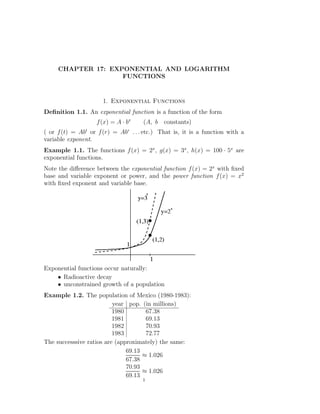
Definition 1.1. An exponential function is a function of the form
f (x) = A · bx (A, b constants)
t r
( or f (t) = Ab or f (r) = Ab . . . etc.) That is, it is a function with a
variable exponent.
Example 1.1. The functions f (x) = 2x , g(x) = 3x , h(x) = 100 · 5x are
exponential functions.
Note the difference between the exponential function f (x) = 2x with fixed
base and variable exponent or power, and the power function f (x) = x2
with fixed exponent and variable base.
Exponential functions occur naturally:
• Radioactive decay
• unconstrained growth of a population
Example 1.2. The population of Mexico (1980-1983):
year pop. (in millions)
1980 67.38
1981 69.13
1982 70.93
1983 72.77
The successsive ratios are (approximately) the same:
69.13
≈ 1.026
67.38
70.93
≈ 1.026
69.13
1
2. 2 First Science MATH1200 Calculus
In each year, the population increases by a factor of 1.026.
Let P (t) denote the population at time t (where t is the number of years
since 1980):
P (0) = 67.38 = P0
P (1) = 67.38 · (1.026)
P (2) = 67.38 · (1.026) · (1.026) = 67.38 · (1.026)2
P (3) = 67.38 · (1.026)3
.
.
.
P (t) = 67.38 · (1.026)t = P0 bt
Thus the estimated population in 1990 is P (10) = 67.38 · (1.026)10 ≈ 87.1
Note: If f (t) = Abt , we get exponential growth if b > 1 and we get expo-
nential decay if b < 1. (b is called the base of the exponential function.)
Example 1.3. Consider the exponential function f (t) = (1/2)t = 2−t :
This function exhibits exponential decay.
Example 1.4. For any given amount of radioactive potassium ( 44 K ),
19
the amount remaining one second later is 99.97%. Find a formula for the
amount at time t. (Let A0 be the amount at time 0).
3. First Science MATH1200 Calculus 3
Solution:
A(t) = amount at time t
A(0) = A0
A(1) = A0 · (0.9997)
.
.
.
A(t) = A0 · (0.9997)t
2. Half-Lives
Suppose that A(t) = A0 · bt with b < 1
(i.e., we have exponential decay).
Then there is a number h > 0 with
1
bh =
2
Thus, if t is any time, the amount at time t + h is
A(t + h) = A0 · bt+h
= A0 · b t · b h
1
= A0 b t
2
1
= A(t)
2
1
= of the amount at time t
2
The number h is called the half-life or 1/2-life of the process.
44
Example 2.1. The 1/2-life of 19 K is 22 mins.
Example 2.2. The 1/2-life of Carbon-14 is 5700 years.
A similar computation shows that if we have exponential growth
A(t) = A0 bt b>1
then bd = 2 for some d > 0.
This number d is called the doubling time for the process.
Example 2.3. The 1/2-life of carbon-14 is 5700 years. Find the formula
for the amount at time t (t in years).
Solution: A(t) = A0 bt . What’s b?
We know
1
A(5700) = A0 b5700 = A0
2
So
1
b5700 =
2
4. 4 First Science MATH1200 Calculus
1
1 5700
=⇒ b = = (0.5)0.000175 ≈ 0.999878
2
So A(t) ≈ A0 · (0.999878)t .
Example 2.4. For a process of exponential decay
A(t) = A0 bt
determine the half-life.
Solution: We must solve
1
bh =
2
for h.
To do this, we need logarithms.
3. Logarithms
The logarithm function answers the question: What power of the number a
is equal to the number c?
Definition 3.1. Suppose that a > 0 and ab = c, then we say that b is the
logarithm of c to the base a and write
loga (c) = b
Example 3.1.
23 = 8 =⇒ 3 = log2 8
104 = 10000 =⇒ 4 = log10 10000
1 1
10−1 = =⇒ −1 = log10
10 10
0
a =1 =⇒ 0 = loga (1)
Thus ‘loga c’ means the power that a must be raised to in order to get c.
Example 3.2. Thus if we ask: What power of 3 is equal to 47? we are
asking for log3 (47). If we ask: what power of 10 is equal to 50?, we are
asking for log10 (50).
Note that the ‘input’ in a logarithm must be a positive number ; i.e., the
domain of the function f (x) = loga (x) is (0, ∞).
Graph of y = log10 x:
5. First Science MATH1200 Calculus 5
Notation: In elementary texts (and in this course), log10 x is simply de-
noted log x , and is called the ‘common logarithm’.
Thus log x = y means 10y = x.
Example 3.3. So log(5) = 0.69897 . . . means 100.69897... = 5.
4. Properties of Logarithms
Theorem 4.1. Fix a > 0.
(1) loga (1) = 0
(2) loga (a) = 1
(3) loga (c1 · c2 ) = loga (c1 ) + loga (c2 )
c1
(4) loga = loga (c1 ) − loga (c2 )
c2
(5) loga (cd ) = d loga (c)
Proof:
(1) Since a0 = 1.
(2) Since a1 = a.
(3) Let b1 = loga (c1 ) and b2 = loga (c2 ). Then ab1 = c1 and ab2 = c2 . So
ab1 +b2 = c1 · c2 (First Law )
=⇒ loga (c1 c2 ) = b1 + b2 = loga (c1 ) + loga (c2 )
(4)
c1 c1
loga (c1 ) = loga · c2 = loga + loga (c2 )
c2 c2
(using 3.).
Now subtract loga (c2 ) from both sides.
(5) Let b = loga (c). So ab = c.
Thus abd = (ab )d = cd (Second Law).
So loga (cd ) = bd = d loga (c)
Note: Taking d = −1 in 5. gives
1
loga = − loga (c)
c
6. 6 First Science MATH1200 Calculus
Example 4.1. The formula for the amount of radioactive polonium is
A(t) = A0 (0.99506)t (t in days )
What is the half-life?
Solution: We need to solve .99506h = 1/2 for h:
log(0.99506h ) = log(1/2)
h · log(0.99506) = log(1/2)
log(1/2)
h =
log(0.99506)
≈ 140 (days )
Thus for a process of exponential decay we have,
log(1/2)
half-life =
log(base)
Similarly, for a process of exponential growth,
log(2)
doubling time =
log(base)
Example 4.2. Estimate the doubling time of the Mexican population.
Solution:
log(2)
d= = 27 (years )
log(1.026)
In general, logarithms are useful for solving equations where the unknown
occurs as an exponent:
Example 4.3. Solve 7x = 231 · 5x for x.
Solution: Take logs of both sides:
log(7x ) = log(231 · 5x )
x log(7) = log(231) + x log(5)
x(log(7) − log(5)) = log(231)
log 231
x =
log 7 − log 5
≈ 16.175
5. Derivatives of logarithms and exponentials
What are
d x d
(2 ) or log(x)?
dx dx
We will not be in a position to answer these questions until we have defined
the natural logarithm function, and to define the natural logarithm we have
to first develop the theory of integration.