SlideShare uma empresa Scribd logo
1 de 33
Baixar para ler offline
from The Complete Computer Hobbyist, ©2005, Donn M. Stewart 132
Designing the Computer
This is the most interesting part of the project. If you are familiar with assembly
language programming, you know that each processor has a characteristic architecture.
The architecture refers to the fixed characteristics that are built into the hardware.
Elements of processor architecture include the size and nature of the instruction set, the
size of the memory address space, the word size, the register structure, and the clock
speed.
As with any engineering project, there are trade-offs in the elements that go into
processor design. A processor with a large data width is more expensive to make, but it
can process faster. The trend toward larger instruction sets and faster clock speeds seen
in the 80x86 series is offset somewhat by RISC (reduced instruction set computer)
processors that have smaller instruction sets, but perform each instruction more quickly.
RISC computers may require longer programs, but with computer memory becoming
very cheap this is not a severe hindrance.
The architecture of a hobbyist computer reflects the goals of the hobbyist. In general, a
computer that works is the primary goal. High performance is very much secondary. A
simple architecture reduces cost, and makes troubleshooting simpler. This increases the
probability of success. Once the hobbyist has successfully built a simple processor, he
may want to build another with higher performance. However, since building a working
processor from scratch is a significant achievement, smaller is better.
I will describe the decisions I made in building my processor. In retrospect, I would have
changed some things. However, this is only after I found that my simple processor
worked, and worked well. My initial design was focused on successful completion, and
not performance.
The most fun I had was designing the instruction set. Here, the hobbyist is completely
free to make his own assembly language. I knew that the earliest computer, the
Manchester Baby, operated with only seven instructions. I thought that it was reasonable
to expand this to sixteen instructions. This meant that four bits of an instruction word
would be taken up by the instruction code. The remainder of the instruction could be an
address, or an operand for arithmetic or logical operations.
The address space of a hobbyist computer may be incredibly small by PC standards. In
the 8-bit microprocessor systems I had built, I used only a hundred or so bytes for
programs and data. I considered a total address space of 256 words for my processor,
which can be encoded by 8 bits, but I opted for the more expansive 12-bit space of 4K
words. This would be very ample for a hobbyist processor.
A 4-bit operation code and a 12-bit address space dictate a 16-bit instruction word size.
This suggests an 8- or 16-bit wide memory. A 16-bit wide memory allows loading of an
instruction in a single step. In retrospect, these choices of opcode, memory space and
word size were optimal.
from The Complete Computer Hobbyist, ©2005, Donn M. Stewart 133
The next decision I made was an error. I decided that the internal data processing
structure of the computer needed to be only 12 bits wide. This would be large enough for
processing integers from 0 to 4K in a single step, and was large enough for address
arithmetic. The program would be in ROM. The program memory would be 16 bits
wide, but the data memory only needed to be 12 bits wide. This would save a little in
complexity and cost. The instructions would cause 12-bit data to be fed to 12-bit
registers, through a 12-bit ALU, and the results returned to 12-bit memory (or output on
12 or 8-bit devices.) The mistake, however, became evident toward the end of the
project. After success seemed assured, I began to daydream of complex software running
on my new machine. Then I realized by mistake: there was no provision for loading
instructions from input to the RAM.
When the computer showed signs of life, I wanted to test it thoroughly. However, this
meant putting even the numerous test programs in ROM, a tedious bit-by-bit process. I
then modified my original design, by adding an extra 4 bits to the accumulator register
and making RAM 16 bits wide. I eventually wrote a ROM program that allowed the
processor to take serial character input from a terminal, translate this into 16-bit
instructions (using a table for the upper 4 bits), and load the instructions in RAM. A
character command would then shift execution to these instructions. The problem of
"dumping" memory output to the terminal was more difficult, since there was no way of
getting the upper 4 bits from the accumulator into the upper 4 bits of an 8-bit character
output. I built a special purpose "byte-switcher" port, which would swap the upper and
lower 8-bits of a word. All this could have been avoided by making the processor 16-bits
wide throughout, which would not have been very difficult...in retrospect.
I wanted a minimal register structure, in part because a 4-bit opcode would not allow for
complex register addressing schemes, and would also be easier to build. A simple
register structure was also important because the part of the computer that contained the
registers could not be tested fully by itself. It could only be tested when the whole
processor was put together. I chose an accumulator-memory model, in which a main
register, the accumulator, serves as the link between the processor and memory. The
accumulator holds one operand of operations such as ADD, and receives the result. The
processor also moves data between memory locations and between memory and input
output by way of the accumulator. In addition to the accumulator, the processor would
also need an instruction register, and a program address register (also called an
instruction pointer, or program counter).
The minimum instruction set for a computer must contain some arithmetic or logical
instructions, memory load and retrieval instructions, and program flow modifying
instructions (jumps), at least one of which must be conditional. The minimal arithmetic
instruction would be subtract, since this allows negation (subtract from zero) and addition
(negation followed by subtraction). A clever programmer might be able to use the
NAND logical operation to derive all the others, including subtract, since this is the root
of all the other operations. However, with computer design, problems are solved by a
combination of hardware and software. A full-function ALU is easy to design, and it
from The Complete Computer Hobbyist, ©2005, Donn M. Stewart 134
seemed that 8 arithmetic/logical instructions (half of the allowed instruction set) would
make a good project. I was confident that I could build such an ALU, and it could be
tested completely on its own. The eight arithmetic/logical instructions I chose were add,
add with carry, subtract, subtract with borrow, NOT, AND, OR, and XOR. I think this
was a good choice.
The rest of the instruction set was available for memory access and flow control
instructions. After some consideration, I decided to have only three memory access
instructions. These were load accumulator immediate (the value is contained in the
instruction itself), load accumulator from memory, and store accumulator to memory.
I now had five spaces in the instruction set left for program flow control. First, there is
the simple unconditional jump. For conditional jumps, I chose jump on carry, jump on
minus and jump on zero. The last spot in the instruction set was filled with an indirect
jump instruction, that is, jump to the location stored in memory. This would allow some
limited subroutine programming, using a memory cell to hold the return address.
In retrospect, it might have been better to have an indexed memory access instruction at
the expense of one of the conditional jumps, or even the jump to memory instruction.
However, indexing could still be done in a roundabout way by incrementing an
instruction in RAM and jumping to it.
With the instruction set completed I now had a basic architecture from which I could
draw detailed plans. The architecture described a processor that had sixteen instructions
and operated on 12-bit data. It would have only one programmer-accessible register, the
accumulator, and would have a 4K word address space. Instructions would be 16 bits
wide, consisting of the 4-bit opcode and a 12-bit operand, which in most cases was an
address. The exceptions were the load accumulator immediate instruction, in which the
operand was a data value, and the NOT instruction, in which the operand was irrelevant.
I somewhat arbitrarily assigned the following operation codes to the instruction set:
Opcode
(binary)
Mnemo
nic
Operand Description
0000 ADD Address of operand Adds the operand to the accumulator, stores
the result in the accumulator
0001 ADC Address of operand Adds the operand and the carry bit to the
accumulator, stores the result in the
accumulator
0010 SUB Address of operand Subtracts the operand from the accumulator,
stores the result in the accumulator
0011 SBC Address of operand Subtracts the operand and the complement of
the carry bit from the accumulator, stores the
result in the accumulator
0100 AND Address of operand Bitwise logical AND of the operand with the
accumulator, stores the result in the
accumulator
0101 OR Address of operand Bitwise logical OR of the operand with the
accumulator, stores the result in the
accumulator
from The Complete Computer Hobbyist, ©2005, Donn M. Stewart 135
0110 XOR Address of operand Bitwise logical XOR of the operand with the
accumulator, stores the result in the
accumulator
0111 NOT None (ignored) Logical bitwise inversion (complement) of the
accumulator, stores the result in the
accumulator
1000 LDI Data Loads the 12-bit operand from the instruction
word into the accumulator
1001 LDM Address of data to be
loaded
Loads a 16-bit data word from memory into the
accumulator
1010 STM Address where data is
to be stored
Stores the 16-bit data word in the accumulator
into memory
1011 JMP Target address to
jump to
Transfers program control to the instruction in
the target address
1100 JPI Address containing
the target address
Transfers program control to the instruction in
the target address
1101 JPZ Target address to
jump to
Transfers program control to the instruction in
the target address, if the 12-bit accumulator
base = 0
1110 JPM Target address Transfers program control to the instruction in
the target address, if bit 11 (leftmost bit of the
12-bit base) of the accumulator = 1
1111 JPC Target address Transfers program control to the instruction in
the target address, if the carry bit = 1
The instruction opcodes for the arithmetic-logical instructions are grouped together from
0000 to 0111. The lower three bits of these opcodes (000 to 111) will serve as a three-bit
ALU opcode. This will simplify the control logic design later on.
The speed of the computer is dictated by the collective speed of the logic gates that need
to change states with each cycle. The cycle time must be long enough to allow the
slowest circuits time to finish operations. The registers, multiplexors and ALU have
pathways of only a few to several dozen gates long. Assuming a gate time of 10
nanoseconds, a cycle time of several hundred nanoseconds would certainly be long
enough. However, the computer memory is also part of the system, and this is usually
the slowest component. I planned to use EPROM chips that had a 400 nanosecond delay
between the request for the data and when it appeared on the outputs. In order to
accommodate this delay, with time to spare, I chose a 1000 ns cycle time, which equals 1
MHz. Slow by modern standards, this is plenty fast enough to give the feel of true
computing.
from The Complete Computer Hobbyist, ©2005, Donn M. Stewart 136
Building the Data Path
The data path of the computer is the ordered collection of registers that hold the data, the
multiplexors that direct the flow of the data, and the ALU that operates on the data. The
memory may also be considered part of the data path, although it is physically separated
from the processor.
Recall the simple machine cycle diagrammed in the previous chapter.
We will start at this point and diagram the processor data path, using as an example the
execution of the ADD instruction. This instruction is executed by the processor in
several steps, each taking exactly one clock cycle to perform. We assume for now that
the processor is running. The mechanism to start the processor will be discussed later.
The ADD instruction that will be executed is part of a larger collection of instructions
that reside in the computer memory. This collection of instructions is the program, and
has been written and placed in the memory by the programmer. Exactly how this is done
will also be discussed later. The computer memory is symbolized by a parallelogram.
D
CP
Q
QClock
Register loads
and displays
results of
previous cycle on
each upward
clock edge
Computer
circuits
perform
operations
on the data
displayed by
the register
from The Complete Computer Hobbyist, ©2005, Donn M. Stewart 137
The memory in our computer will be 16 bits wide, and at present will be shown with
distinct data inputs and outputs. The memory address is specified a 12 bit input.
We will assume for now that the memory acts like a large collection of registers in that a
rising clock pulse edge at the Memory Write input will cause the data on the inputs to be
loaded into the memory cell specified by the address. This data will then appear on the
outputs. In the absence of a Memory Write pulse, the memory will simply display
whatever data is present in the memory cell specified by the address input. The Memory
Write signal will be derived from the processor control logic that will be described later.
It is a single bit input.
The first step in executing the ADD instruction is to get the instruction from memory.
This is commonly called the instruction fetch step. Since the processor is running, it
contains in the Program Counter register the address of the ADD instruction we want to
fetch and execute. To get the ADD instruction out of memory, we simply send the output
of the Program Counter register to the memory address inputs.
After a few hundred nanoseconds, still well within the limits of one clock cycle, the
desired instruction will appear on the memory data output lines. However, in order to
execute the instruction we need to save it somewhere. We cannot simply keep it on the
memory output lines, since we will need to get at least one of the ADD operands from the
memory (the other operand is already in the accumulator register, left there by prior
instructions). We will store the instruction in the Instruction Register.
Memory
Memory
16 16
Data in Data out
12
Address
Memory Write
from The Complete Computer Hobbyist, ©2005, Donn M. Stewart 138
All of the registers, like the memory, have Write inputs. To complete the instruction
fetch cycle, we need to send an Instruction Register Write pulse to the Instruction
Register. This pulse, like all the other register write signals, will come from the control
logic, to be designed later. We now have diagrammed all the parts of that data path
needed to complete the instruction fetch.
After the instruction fetch, the computer will need to prepare itself to get the next
instruction. Unless a jump instruction is being executed, the next instruction is in the
memory cell immediately following the one just fetched. Therefore, we need to increase
the value of the program counter by one. How can we do this?
The answer is simple. We will have an ALU built into the processor, and it has nothing
to do in the first part of the instruction fetch. Why not use it to add 1 to the Program
Counter? The ALU can do this while the memory is getting the current instruction. By
the time the current instruction is ready to be clocked into the instruction register, the
incremented program counter is ready to be clocked into the PC register. Remember, we
are using rising clock edge triggered registers, and the increased Program Counter value
will not appear on the Program Counter Register outputs until the program counter write
pulse arrives. This will happen at exactly the same time that the instruction register write
pulse arrives at the instruction register. There will not be enough time for the new
program counter value to confuse the system with another instruction, since the
instruction register will be closed for inputs long before the new instruction appears on
the memory data output. Until we send another IR write pulse during the fetch phase of
the following instruction execution, the current ADD instruction will abide securely in
the Instruction Register.
Here is a diagram showing how we can use the ALU to increment the Program Counter.
Remember the diagram of the ALU from previous chapters. Our ALU will process 12
bits and have a three-bit opcode.
16 16
Data
in
Data
out
12
Address
Program
Counter
Instruction
Register
Instruction
Register Write
Program
Counter
Write
from The Complete Computer Hobbyist, ©2005, Donn M. Stewart 139
We do not use the carry in when the program counter is incremented. All we have to do
is send the current Program Counter value to one input of the ALU, the 12-bit number 1
to the second (that is, binary 0000 0000 0001), and put the three bit ADD opcode on the
ALU opcode inputs. After a short delay, the incremented Program Counter will appear at
the ALU output and will be sent to the Program Counter inputs. It will wait there until
the Program Counter Write pulse arrives, at which point the incremented program
counter value will be loaded into the register, ready to fetch the next instruction.
We have finished putting together the pathway for the instruction fetch and the program
counter incrementation step. I will add to the diagram as we go through the rest of the
ADD instruction execution. In order to make room in the diagram, I will not show the
number of bits in each connection, nor the register write inputs from now on to reduce
clutter.
12
12
12
1
Program Counter
ADD Opcode
Opcode
Output
Carry-in
Carry-Out
A input
B input
3
12
12
12
from The Complete Computer Hobbyist, ©2005, Donn M. Stewart 140
At the end of the instruction fetch/program counter incrementation cycle, the Program
Counter Write and Instruction Register Write inputs receive clock pulses. The rising
edge of these clock pulses locks the results of this cycle into these registers at the same
instant, and then the next cycle begins. In the diagram, I show that the upper four bits of
the IR holds the instruction opcode, and the lower 12 bits the instruction operand. These
two parts of the IR are sent on different paths, as I will show soon.
The next clock cycle is Instruction Interpretation. During this cycle, nothing happens in
the data path. The instruction opcode (the upper 4 bits of the instruction register) is sent
to the control logic. This opcode, along with the zero, minus, and carry condition flags,
directs the control logic to set the control lines of the data path in such a way as to carry
out the operation desired. In order to perform the ADD operation, the control logic will
cause the data path to perform the following two steps, each taking one clock cycle.
First, an operand stored in the memory will be fetched and placed in the Data register.
Second, the Accumulator and Data register values will be sent to the ALU data inputs,
and the three-bit ALU opcode for ADD will be sent to the ALU opcode input. At the end
of this second step, on the rising edge of the next clock pulse, the ALU output will be
stored in the Accumulator and the carry-out will be stored in a one-bit carry flip-flop.
When the ADD operation is complete, the control logic will instruct the data path to
begin another instruction fetch/program counter incrementation cycle, and execute the
next instruction found in the computer memory.
We need to expand our drawing of the data path to show the other registers and pathways
involved in the ADD operation. First, we will add the components needed for the Data
Register fetch step.
PC Memory IR
ALU
1
Opcode (bits 12-15)
Operand (bits 0-11)
Address in
Data
out
Data in
Add
from The Complete Computer Hobbyist, ©2005, Donn M. Stewart 141
Notice that I added the Address Source Multiplexor to select the source of the memory
address for the operand fetch. During the instruction fetch, the Program Counter held the
address of the instruction. Now, the Instruction Register holds the address of the data to
be placed in the Data Register for addition. Of course, the multiplexor input is selected
by a signal from the control logic. At the end of this data fetch cycle, a register write
pulse is sent by the control logic to the Data Register, but no write pulse is sent to the
Instruction Register. This ensures that the Instruction Register will continue to hold the
ADD instruction that was fetched earlier.
During the final cycle of the ADD instruction, the contents of the Accumulator and Data
registers are directed to the ALU inputs, along with the ADD opcode contained in the IR
bits 12-14. After a short delay, the result of the addition will appear on the ALU output.
This result will be clocked into the accumulator register by a write pulse at the end of the
cycle. The carry-out bit will also be stored in a flip-flop. We will now add the
Accumulator register and a few more elements to the data path diagram.
PC
Address
source
multiplexor
Memory IR
ALU
0
1
Add
Data register
Op-
code
Oper-
and
Addr
Data
out
Data in
PC = Program Counter
IR = Instruction Register
1
from The Complete Computer Hobbyist, ©2005, Donn M. Stewart 142
We need ALU source multiplexors to send the proper inputs to the ALU. In the Program
Counter Incrementation step we sent the Program counter to the ALU A input, and the
12-bit value 1 to the ALU B input. In all the two-input arithmetic and logical
instructions, such as ADD and OR, we will send the Accumulator to the ALU A input,
and the Data Register to the ALU B input. We also need to add a multiplexor to select
the ALU operation, either the stand-alone ADD operation for the PC incrementation step,
or the ALU opcode contained in bits 12 to 14 of the Instruction Register.
Notice how the ALU output is connected to both the Accumulator and Program Counter
inputs. At the end of the last cycle of execution of the ADD instruction, the control logic
sends a write pulse to the Accumulator and carry flip-flop. No write pulse is sent to the
Program Counter, so it remains unchanged. After this final write pulse, the Accumulator
will contain the result of the addition, and the Carry flip-flop will contain the carry-out
bit.
The data path diagrammed above is adequate for the instruction fetch/program counter
incrementation cycle, and for all the arithmetic-logical operations except those using a
carry-in (or borrow). To finish the data path for the arithmetic instructions that need a
carry input, we add a path from the output of the Carry flip-flop to the ALU carry-in.
Whether the carry-in is used or not depends on the ALU opcode, so there is no control
line for this outside the ALU.
PC
Address
source
multiplexor
Memory IR Accumulator
ALU source
multiplexors
A
B
ALU
ALU Op
source
multiplexor
0
0
1
Add
0
1
0
11
Data register
1
Op-
code
Oper-
and
Addr
Data
out
Data in
PC = Program Counter
IR = Instruction Register Carry FF
from The Complete Computer Hobbyist, ©2005, Donn M. Stewart 143
We now have a data path that will perform all eight of the arithmetic-logic instructions in
our instruction set. A few more modifications will allow the other eight instructions to be
performed.
To perform the load/store instructions, connections between the accumulator and the
memory are needed. There is only one type of store instruction, that is, store accumulator
to memory (STM). However, there are two types of load instructions: load accumulator
from memory (LDM), and load accumulator immediate (LDI). In the LDM (memory)
load, the accumulator gets its input from the memory; the memory address is in the lower
12 bits of the instruction register. In the LDI (immediate) load, the value itself is in the
instruction register. Therefore, we need an Accumulator Source Multiplexor to select the
appropriate accumulator input: the ALU (from the arithmetic-logic instructions), the
memory (LDM) or the instruction register (LDI).
PC
Address
source
multiplexor
Memory IR Accumulator
ALU source
multiplexors
A
B
ALU
ALU Op
source
multiplexor
0
0
1
Add
0
1
0
11
Data register
1
Op-
code
Oper-
and
Addr
Data
out
Data in
PC = Program Counter
IR = Instruction Register Carry FF
from The Complete Computer Hobbyist, ©2005, Donn M. Stewart 144
This data path is able to execute the instruction fetch/program counter step, the arithmetic
logical instruction steps, and the memory load/store instruction steps. The remaining
instructions are the program flow, or jump instructions. These instructions operate by
placing into the program counter a new value, either from the memory (indirect jump) or
from the instruction register (direct jumps). Therefore, we need connections between the
instruction register and the program counter, and the memory and the program counter.
This means we need a PC source multiplexor to select the proper PC input. The
conditional jumps in our limited instruction set are direct jumps, and whether they are
executed or not depends the value of the carry flip-flop (jump on carry) or the value of
the accumulator (jump on zero, or jump on minus). No extra connections are needed
beyond those for the unconditional jumps. If the condition is met, the control logic will
cause the (direct) jump to occur, and if not it will simply cause the data path to fetch the
next instruction in memory, skipping the jump step.
Carry FF
PC
Address
source
multiplexor
Memory IR
Accumulator
source
multiplexor Accumulator
ALU source
multiplexors
A
B
ALU
ALU Op
source
multiplexor
0
0
1
0
1
2
Add
0
1
0
11
Data register
1
Op-
code
Oper-
and
Addr
Data
out
Data in
PC = Program Counter
IR = Instruction Register
from The Complete Computer Hobbyist, ©2005, Donn M. Stewart 145
This completes the data path for the computer. There are some details that need to be
added. Extra logic is needed in order to work with real computer memory that doesn't
write like a register. This topic deserves its own section, which will follow. Also, some
simple logic (11 two-input OR gates) is needed to derive the accumulator zero signal (the
accumulator minus signal is simply the uppermost bit in the register). If you can
understand the diagram above, you are well on your way to understanding a real
computer at its most fundamental level.
This data path can be built with standard IC components of the 74LS00 series.
Specifically, there is an IC that has an 8-bit register in a 20-pin package, and two of these
will do for the instruction register. Similarly, three 6-bit register IC's will make a 12-bit
register. The 12-bit 4 input multiplexors can each be built of 6 dual one-bit multiplexor
IC's, and the one-of-two multiplexors can be built from IC's that have four single-bit one-
of-four multiplexors per chip. To make the zero logic, a 12-input OR gate can be used,
made from 11 2-input OR gates on 3 IC's. One chip with the carry flip-flop is also
needed. The total number of IC's needed for this data path is 34, and would cost about
$17.00. Of course, the sockets and board increase the cost up to about $50.00.
Carry FF
PC
PC source
multiplexor
Address
source
multiplexor
Memory IR
Accumulator
source
multiplexor Accumulator
ALU source
multiplexors
A
B
ALU
ALU Op
source
multiplexor
0
0
1
2
0
1
0
1
2
Add
0
1
0
11
Data register
1
Op-
code
Oper-
and
Addr
Data
out
Data in
PC = Program Counter
IR = Instruction Register
from The Complete Computer Hobbyist, ©2005, Donn M. Stewart 146
Real Computer Memory
As mentioned in the previous section, real computer memory does not operate like a large
collection of data registers. There are two main differences. First, the memory write
process is more complicated, involving several signals that have to be created by the
computer logic. Second, memory uses a bi-directional data path, called a data bus.
The semiconductor RAM memory circuit I used in this computer is 4-bit by 1K static
random access memory (SRAM), specifically the 2114 IC. Static RAM does not require
refreshing every millisecond or so like the cheaper, faster dynamic random access
memory (DRAM). It is important to build your hobbyist computer with SRAM, because
in the troubleshooting phase of construction you will need to run it very slowly, one cycle
at a time, in order to find out why it is not working. DRAM will not function in a single
step cycle, unless it has its own clock circuit. An additional benefit of using SRAM is
that you don't have to create the circuitry to perform the refresh cycles during normal
operations. Now, one can buy DRAM with the refresh circuitry built in, called SDRAM.
However, our computer uses so little RAM, that it makes sense just to use the old-
fashioned 1K 2114 circuit. It is all the RAM you will ever need.
The memory is written with the help of two inputs. The first is the chip select (CS) input,
which must be made low (0 V) in order for the chip to function, either for input or output.
The other input is the write input (WR). This input must be made low, and held low for a
specified minimum time. During this time, the address and data on the memory inputs
must be held steady. At the end of the required time span, the write input is made high
(5V), and the data is locked into the memory.
The key factor in the timing is that the memory write input must go high before the
address or data inputs change, in order to ensure that the data is safely written. This
presents a problem for the computer designer. He (or she) would like to write to the
memory in a single cycle. However, at the end such a cycle, the address, data and
memory write signals would all change at approximately the same time, putting the data
in some peril. You might try to chance it, but there is a better way.
The answer is to spread the memory write over two clock cycles. This gives us some
additional clock edges with which to work. We can now ensure that the memory write
goes high well before the data or address inputs have a chance to change.
Here is the kind of timing we would like for a solid memory write:
from The Complete Computer Hobbyist, ©2005, Donn M. Stewart 147
Each figure above represents the voltage level on the indicated memory inputs, or the
clock. The memory write process proceeds this way. At the start of the first memory
write clock cycle, A in the diagram, the processor puts the address of the memory
location to be written on the address inputs of the memory. Simultaneously, the chip
select memory input is made active (low) since this memory control input is derived
directly from the address. One-half cycle later, on the downward edge of the clock in
cycle A, the Memory Write (WR) is made active (low). At the beginning of the B cycle,
the data is placed on the memory inputs, and on the downward edge of the clock in the B
cycle, the WR input becomes inactive (high). At this point, the data is locked into the
memory. At the end of the B cycle, on the upward clock edge of the next machine cycle,
the address used during the memory write, and the derived CS input, are inactivated. The
address, CS, data and WR are all active during the first half of the B cycle, which lasts
500 nanoseconds for a 1 MHz clock. This easily meets the minimum time requirement
for writing the 2114 memory chip, which is about 200 ns.
It is not hard to make a circuit that will provide the proper timing of the memory write
input (WR). Here it is:
Time
Voltage
A B
System Clock
Memory Write
Chip Select
Address for
memory write
Data for
memory
write
Not ready Ready Not ready
Not ready Not readyReady
0
CP
D Q WR to memory
System Clock
Memory Write
(from control logic)
from The Complete Computer Hobbyist, ©2005, Donn M. Stewart 148
This is simply an edge-triggered flip-flop whose clock pulse input is the inverted system
clock. The control logic Memory Write signal comes on (becomes one) at the beginning
of the A machine cycle, in response to the program instruction STM. However, since the
flip-flop has an inverted clock signal, it is not written into the flip-flop until the middle of
the A cycle. That is, when the clock has a falling edge in the A cycle, the inverted clock
input to the flip-flop will have a rising edge, and the Memory Write signal will be written
into the flip-flop. It then appears on the output, and is inverted. This output is connected
to the WR input on the memory chip (the WR signal to the memory chip is active when
low.) When the WR memory input goes low, the memory begins to store the data that
the processor has placed on its inputs. The Memory Write signal from the control logic
goes to zero at the end of the machine cycle A, but since the flip-flop has an inverted
clock input, the WR output is held low for another half-cycle, giving the memory the
time it needs to finish storing the data. In the middle of the B cycle, the flip-flop sees a
rising clock edge from the inverted clock input, and stores the Memory Write zero. The
WR now goes to 1, and the memory write is finished.
The timing diagram shows the requirements for writing a real semiconductor memory
with the various control inputs. The other feature of memory, that makes it different
from a register, is that it has bi-directional data input/output lines. These lines are
controlled by a device called a three-state buffer, which I will now describe.
Recall that a computer consists of large networks of automatic switches, each of which is
either on (logical 1, or 5V) or off (logical 0, or 0V). But remember, that in order to be
either 5 or 0 volts, an output has to be connected, through the logic gate circuit, to either
the 5V or 0V (ground) power supply leads of the gate. What would be the state of an
output that was connected to neither? That is, pretend you cut the output wire, and it is
hanging in the air.
Remember that the output voltage of a logic circuit is only part of an output. The other is
the ability to pass current. So, if an output is 5V, it also needs to be able to pass some
current to drive inputs of other gates to which it is connected. Similarly, if an output is
0V, it needs to be able to "sink" current, in order to operate the circuits it is tied to. The
"cut wire" state is a third state, neither 1 nor 0, that is very useful in computer system
design. The third state is also called "high impedance", because current will not be able
to flow either into or out of an output that is in this state. The high impedance state can
also be thought of as having a very high resistance. It is shortened to "Hi Z". Here is a
simple switch diagram that shows a two-state and a three-state device.
1000 ohms
Two-state output
from The Complete Computer Hobbyist, ©2005, Donn M. Stewart 149
In the upper diagram, the switch can be open or closed. This type of switch is called a
single-throw switch. If open, the output is connected through the resistor to ground, and
will have a voltage of 0 with ability to sink some incoming current to ground through the
resistor. When the switch is closed, the output will be 5V, with the ability to pass
significant current to outside devices. The lower diagram shows a switch that can have
three positions; closed to the 5V contact, open in the middle, or closed to the grounded
contact. Such a switch is called a double-throw switch. Note that the circuit output is
connected to the central pole of the switch. The middle position is the third state. It is
just like a cut wire. The output, connected to the central pole of the switch, will not be
able to conduct any current anywhere with the switch in the middle position and its
voltage will be undefined. This is characteristic of the third, or high-impedance state.
Having a three-state logic device output allows us to take a huge short cut when we
assemble a true computer system. It allows us to use a collection of wires to pass data in
two different directions. A collection of parallel wires is called a bus, and when it can
pass data in two directions it is called a bi-directional bus.
The bi-directional bus allows us to connect many separate devices that have three-state
outputs to the same set of wires, and then use logic to select which devices will
communicate to each other. The other unselected devices will remain in the third state,
and will be invisible to the active circuits. They will not interfere with the data
communications between the active devices. We are bringing this up here, because
computer memory is such a device, with three-state data outputs. When the memory
write signal is given to a selected memory chip, the outputs behave as data inputs, in
order to write data in the memory. When the memory write signal is inactive, the outputs
behave as outputs, sending data onto the bus. When the chip is not selected, the outputs
are in the third, high-impedance state, and the chip is invisible to other devices on the
bus, such as input or output ports. It is convenient to think of the memory data lines as
input/output lines, because they can change direction.
It is a simple matter to make a bi-directional bus using three-state logical devices. The
two most commonly used are the three-state buffer, and three-state inverting buffer.
Switch contact swings both ways
Three-state output
from The Complete Computer Hobbyist, ©2005, Donn M. Stewart 150
The control input is a signal that enables the gate to pass data when it is on (1). The
control input is sometimes called an enable input. Here is how to make a bi-directional
buffer out of two three-state buffers and an inverter.
When control is 1, the data flows from A to B, and when it is 0, from B to A. In other
words, when control is 1, A is the input and B is the output, and when control is 0, B is
the input and A is the output. Thus A and B are input/outputs.
Inclusion of another control can allow the bi-directional buffer to go to the Hi Z state.
This type of circuit is used inside memory circuits to control the input/output lines
Input Output
Input Output
Control input
Control input
In Control Out
0 0 Hi Z
1 0 Hi Z
0 1 0
1 1 1
In Control Out
0 0 Hi Z
1 0 Hi Z
0 1 1
1 1 0
B
A
Control
A
Control
B
Select Control Direction
1 0 B to A
1 1 A to B
0 0 Hi Z
0 1 Hi Z
Select
from The Complete Computer Hobbyist, ©2005, Donn M. Stewart 151
In the data path defined in the previous section, we are faced with the problem of how to
connect a register, with separate inputs and outputs, to a memory chip with bi-directional
three-state input/outputs. First of all, the problem really only occurs during the memory
write cycle, because otherwise the memory is either putting out data (if selected) or is in
the high impedance state (if not selected). If the memory input/outputs are directly
connected to register inputs, both of these conditions are tolerable. However, the register
outputs cannot be connected directly to the memory input/outputs, because when the
memory is in the output condition, you will have memory outputs connected to register
outputs, which is not tolerable. We will use a three-state buffer to prevent the register
outputs from being connected to the memory input/outputs as long as the memory is in
the output condition. The circuit is simple:
The three-state buffer protects the memory outputs from colliding with the register
outputs when the memory is in the output mode. When the memory goes into the input
mode, and the memory input/outputs become inputs, then the Data out control signal
comes on, and the three-state buffer becomes an output. In the timing diagram shown
earlier, this takes place at the beginning of the B machine cycle. Note that using a three-
state buffer to make a bi-directional data bus doesn't bother the register at all; its inputs
are always connected to outputs, regardless of whether the memory is in input or output
mode.
Here is a diagram of the data path with the three-state data out buffer included. Now, the
memory input/outputs are connected to a bi-directional data bus.
CP
D Q
Bi-directional data bus
Memory
Register
Register write
pulse
Three-state buffer
Data out to memory
from The Complete Computer Hobbyist, ©2005, Donn M. Stewart 152
The only devices capable of putting an output on the data bus are the accumulator (during
a memory write) and the memory (most of the rest of the time). The other devices
(multiplexors and registers) are always inputs. Inputs don't interfere with bus traffic.
We can put other devices on the bus, such as input/output ports. Any device that places
data onto the bus, like an input port when active, will need to have three-state outputs.
Then, we can read from or write to ports as if they were memory locations, using memory
load or store instructions. The only difference is that the numbers we write will affect the
devices attached to the port. This is how we will connect our computer to the outside
world. It is the address in the instruction that will activate either the memory, or the
ports. As long as the devices that place data onto the bus have three-state outputs, and as
long as we avoid colliding outputs by proper logic, there is no limit to the number of
devices that can use the bus.
Carry FF
PC
PC source
multiplexor
Address
source
multiplexor
Memory IR
Accumulator
source
multiplexor Accumulator
ALU source
multiplexors
A
B
ALU
ALU Op
source
multiplexor
0
0
1
2
0
1
0
1
2
Add
0
1
0
11
Data register
1
Op-
code
Oper-
and
Addr
Data in
or out
PC = Program Counter
IR = Instruction Register
Three-State Data out buffer
Bidirectional Data Bus
from The Complete Computer Hobbyist, ©2005, Donn M. Stewart 153
The Machine within the Machine--Control Logic
The data path described in the previous chapter is the tool kit of the computer. The
registers and multiplexors, together with the ALU and the memory, have the power to
perform all the operations of the instruction set we designed earlier. However, it is the
control logic that really runs the computer. It coordinates and controls all the data path
elements. The control logic takes as its input the instruction operation code, and
generates a sequence of outputs that causes the data path to manipulate data or alter the
flow of the computer program.
For each instruction, the control logic defines a series of steps. With each step, the
control logic generates specific outputs. These outputs are fed to the data path
multiplexor and register write inputs. Each step of the sequence is designed to be
performed in a single clock cycle. If we want to perform a task that does not fit into one
clock cycle, we need to break it up into sub-steps. The control logic keeps track of these
steps by assigning a unique number to each one, called the state. The state is kept in a
register in the control logic circuitry.
A device that uses a finite number of states in specified sequences to control a process is
called a finite state machine. The machine works as follows. The cycle starts at some
initial entry state, which we will assign the number 0. This value is placed into the state
register. The control logic then looks at the state register and the current instruction
opcode. Using standard AND/OR logic gates, it then creates two outputs. One output is
the pattern of 1's and 0's that is sent to the data path elements (multiplexors and registers)
to perform data and program flow manipulations. The other output is the next state. At
the end of the clock cycle, the next state is written into the state register. At this point,
the next state becomes the current state for the next cycle.
Control
Logic
State register
Clock
Control output to Data
Path
Next State output
to state register
Current State input
from state register
Instruction Opcode
input from instruction
register
from The Complete Computer Hobbyist, ©2005, Donn M. Stewart 154
The state register is written every clock cycle, and therefore the computer clock is
directly connected to its write input.
Different instructions can use the same states. For example, all instructions will start
with state 0, which is the instruction fetch/program counter incrementation step. This
will always be followed by state 1, which is the instruction interpretation step. If the
processor is executing an arithmetic/logic instruction that has two operands, it will use a
data fetch step. All arithmetic/logic instructions can use the same state for the data fetch
step. The arithmetic/logical instructions that write the carry flip-flop can all use the same
state, and the ones that do not can all use the same state. When the final state of a
sequence is finished, the next state logic will give a 0 as its output, and a new sequence
will start. Once the sequence of states is built into the control logic, the cycle operates
endlessly.
How many states are required? Our instruction set has 16 operations, and each operation
will need from 2 to 4 steps (or states) to operate. However, many states are shared by
several operations, and this reduces the total number of states required. In fact, our
computer can be built with a control logic that uses only 11 states (0 to 10). Modern
complex instruction set processors, such as the Pentium, need hundreds of states.
By looking at the data path diagram, and thinking about what needs to happen in order
for an instruction to be carried out, we can make a list of the states that will do everything
our instruction set needs to do. Here are the states for this processor. The numbers we
assign are somewhat arbitrary, although it is important to make state 0 the first step. This
allows us to use a simple circuit to start the computer.
State Action
0 Instruction fetch/program counter incrementation
1 Instruction interpretation
2 Data fetch
3 Arithmetic instruction, includes carry write
4 Logic instruction, no carry write
5 Load accumulator immediate (value in current instruction)
6 Load accumulator from memory
7 Store accumulator to memory, first step
8 Store accumulator to memory, second step
9 Jump immediate
10 Jump indirect
By referring to these states, we can now associate each instruction in our instruction set
with the sequence of states needed to carry it out. We have already shown how the
sequence of states 0,1,2,3 will perform the ADD operation. Here is the complete
instruction set with the corresponding state sequences.
from The Complete Computer Hobbyist, ©2005, Donn M. Stewart 155
Instruction Opcode Condition Opcode Mnemonic State sequence
0000 ADD 0,1,2,3
0001 ADC 0,1,2,3
0010 SUB 0,1,2,3
0011 SBC 0,1,2,3
0100 AND 0,1,2,4
0101 OR 0,1,2,4
0110 XOR 0,1,2,4
0111 NOT 0,1,4
1000 LDI 0,1,5
1001 LDM 0,1,6
1010 STM 0,1,7,8
1011 JMP 0,1,9
1100 JPI 0,1,10
1101 Z = 0 (not zero) JPZ 0,1
1101 Z = 1 (zero) JPZ 0,1,9
1110 M = 0 (not minus) JPM 0,1
1110 M = 1 (minus) JPM 0,1,9
1111 C = 0 (not carry) JPC 0,1
1111 C = 1 (carry) JPC 0,1,9
Notice that the arithmetic operations all use the same sequence of states. The difference
between addition and subtraction, and the use of the carry-in, depends on the three-bit
ALU opcode that is imbedded in the instruction opcode, so we do not need separate states
for each. Similarly, the logical operations share the same sequence, the difference being
that state 5 does not write the carry-out to the carry flip-flop. The NOT operation, which
does not have a second operand, skips the data fetch state. The conditional jump
instructions use the same state sequence as the unconditional direct jump when the
corresponding condition is met. If the condition is not met, the direct jump state is
simply omitted and the instruction performs no operation at all. Since each state is one
clock cycle long, we can tell how long each instruction will take to execute. If we
assume a clock rate of one megahertz, then the processor should be able to execute an
addition (or any other 4-state instruction) in 4 microseconds.
We will create the control logic so that the control output depends only on the current
state. There are other ways to do this, such as making the control output for the
conditional jumps depend on the condition, but I think this way is simpler. I will now
show a table of the control outputs that correspond to each state. There is one control
output for each data path control input. Note that a three-input multiplexor needs two
control inputs, for the low order and high order bits (bits 0 and 1). Refer to the data path
diagram for the elements that use control inputs.
from The Complete Computer Hobbyist, ©2005, Donn M. Stewart 156
Control input State
0 1 2 3 4 5 6 7 8 9 10
Program Counter Multiplexor Low 1 X X X X X X X X 0 0
Program Counter Multiplexor High 0 X X X X X X X X 0 1
Program Counter Write 1 0 0 0 0 0 0 0 0 1 1
Memory Address Multiplexor 1 X 0 X X X 0 0 0 X 0
Memory Write 0 0 0 0 0 0 0 1 0 0 0
Memory Data Out 0 0 0 0 0 0 0 0 1 0 0
Instruction Register Write 1 0 0 0 0 0 0 0 0 0 0
Accumulator Multiplexor Low X X X 0 0 1 0 X X X X
Accumulator Multiplexor High X X X 0 0 0 1 X X X X
Accumulator Write 0 0 0 1 1 1 1 0 0 0 0
Data Register Write 0 0 1 0 0 0 0 0 0 0 0
ALU A Multiplexor 1 X X 0 0 X X X X X X
ALU B Multiplexor 1 X X 0 0 X X X X X X
ALU Operation Multiplexor 1 X X 0 0 X X X X X X
Carry flip-flop Write 0 0 0 1 0 0 0 0 0 0 0
X = don't care
Notice that we don't care what the multiplexor control inputs are if we are not going to
write the registers (or memory) whose input is supplied by that multiplexor. The "don't
cares" allow us to design the logic more efficiently. Also, note that some of the control
lines behave identically across all states. It is easy to see that the ALU A and B
multiplexor control lines, and the ALU operation multiplexor control line could all be
replaced by a single control line. Other control lines might also be consolidated, such as
the program counter multiplexor low and the instruction register write. However, I felt
that extensive consolidation of control lines might be confusing when it came to
troubleshooting the processor, so I only consolidated the ALU multiplexor lines. It is
more important to minimize the number of states needed. In the control design above, no
two states can be consolidated.
In order to make a circuit that will "map" one state to one control output we have two
main options. The option used by most processor manufacturers is to use microcode.
The microcode technique uses a read-only memory to hold the control output
configurations, in the form of binary numbers. The control output for each state in the
above table could be considered as a 15-bit binary number. We can store the control
output configuration for each state in such a way that Carry Flip-Flop Write is in the
rightmost (low) bit, and the Program Counter Multiplexor Low is in the leftmost (high)
bit. If we replace the don't cares with 0, then the control line output for state 0 would be
the binary number 101 1001 0000 1110. The control line output simply becomes a 15-bit
wide memory with 11 locations, one for each state.
from The Complete Computer Hobbyist, ©2005, Donn M. Stewart 157
For the hobbyist, this arrangement is attractive because the control output function can be
changed without rewiring circuits. However, it requires the programming of ROM, and
this requires extra equipment. But it is likely that you will need a PROM programmer
anyway, so it is reasonable to consider this.
The other way to make a circuit that "maps" a state onto a control output is to use a
decoder, together with AND-OR logic. In this method, the control output for each state is
hard-wired into the board. If you like to wire things up, this is the way to go, and this is
the way I did it.
Without showing the whole circuit, here is an example of how the states might be
decoded into the corresponding control outputs
Program Counter Multiplexor Low
Program Counter Multiplexor High
Program Counter Write
Memory Address Multiplexor
Memory Write
Memory Data Out
Instruction Register Write
Accumulator Multiplexor Low
Accumulator Multiplexor High
Accumulator Write
Data Register Write
ALU A Multiplexor
ALU B Multiplexor
ALU Operation Multiplexor
Carry flip-flop Write
The 4-bit state value is placed on the decoder inputs, and the corresponding output
becomes 1. The other outputs are 0. The Program Counter Write and Accumulator Write
control lines are on in several different states, so multiple input OR gates are required to
provide these outputs. The other control lines are connected directly to only one state
output. If you compare this circuit with the table on the previous page, replacing the X
0 21 3 54 6 7 98 10
Four-to-sixteen state decoder
4-bit State input
(from state register)
from The Complete Computer Hobbyist, ©2005, Donn M. Stewart 158
don't cares with zeros, you can see that this simple circuit faithfully provides the
appropriate control outputs. This circuit can be built with one 4-to-16 decoder and 6 two-
input OR gates, a total of 3 IC's. The control logic is half done.
The other function of the control logic is to provide the sequence of states for each
instruction. We call this the next-state function. The next-state function circuitry takes
as its inputs the current state, the current instruction, and the conditions (zero, minus and
carry). From these inputs, the next state is determined.
The next-state function circuit is more difficult to design than the control output circuit.
This is because it has a much more complex input. If we count each bit of the current
state, current instruction and conditions, there are 4 + 4 + 3 = 11 bits of input, instead of
the 4 bits of input to the control output circuit. Eleven bits can encode over 2,000
different combinations instead of the 16 handled by the simple decoder-based circuit we
used for the control outputs.
Of course, not all these combinations are used, and although there are 16 instructions
there are only 11 states. Also, some instructions use the same sequence of states, and
most don't care about the condition flags. Nevertheless, the next state function design
requires some thought.
As with the control outputs, a microcode contained in a programmable ROM could also
provide the next state function. The current instruction, current state and condition flags
could be used to form an address, and the output would be the next state. In fact, the
control output and next state function could be combined into a single PROM, with an
11-bit address and 19-bit output (4 bits for the next state, 15 bits for the control outputs).
A more elegant way to encode the next state function is to use the technique of AND-OR
arrayed logic. This type of logic is able to encode any function that maps an input to a
unique output. With the inclusion of inverters, arrayed logic has the power to perform all
the functions of the digital computer. In fact, programmable array logic IC's can be used
to create entire microprocessors. We already saw an example of AND-OR array logic in
the chapter about building the ALU.
In our case, we will first diagram the next state function as an AND-OR array, and then
show how to build it. Keep in mind that the AND-OR array diagram is not a circuit
diagram, but only a plan that will allow us to build the actual array.
The diagram consists of two parts. The upper part shows how the inputs are connected to
multiple input AND gates. The lower part shows how the outputs of these AND gates are
connected to multiple input OR gates. The OR gate outputs are the outputs of the circuit,
the next state value.
The first step in creating the next state operation is to map it out in a table. This will
show us what we need to do when it comes to building the circuit. We will list all
possible combinations of current state, current operation and condition flags, and the
from The Complete Computer Hobbyist, ©2005, Donn M. Stewart 159
corresponding next state. First, we will make the table with decimal values for the states,
using the mnemonics for the operations.
Current state Operations Condition Next state
0 Don't care Don't care 1
1 ADD, ADC, SUB, SBC, AND, OR, XOR Don't care 2
1 NOT Don't care 4
1 LDI Don't care 5
1 LDM Don't care 6
1 STM Don't care 7
1 JMP Don't care 9
1 Conditional jumps Condition met 9
1 Conditional jumps Condition not met 0
1 JPI Don't care 10
2 ADD, ADC, SUB, SBC Don't care 3
2 AND, OR, XOR Don't care 4
3 Don't care Don't care 0
4 Don't care Don't care 0
5 Don't care Don't care 0
6 Don't care Don't care 0
7 Don't care Don't care 8
8 Don't care Don't care 0
9 Don't care Don't care 0
10 Don't care Don't care 0
The "don't care" entries show which states are always followed by the corresponding next
state, regardless of the operation or condition.
The above table must be made into a circuit. In order to do this, we will need to look at
the binary representations of the current state, operation and condition, and figure out
how combine them to make a binary representation of the next state using AND-OR array
logic.
It is convenient to think backward in making the AND-OR array. In other words, we
look at each bit of the next state, and ask what kind of AND-OR operation is needed to
get it from the corresponding current state, operation and condition as listed in the table
above. Let us label the next state bits NS0 to NS3, (from low bit to high bit.) We will
create operations that will cause the next state bit in question to become 1 when the input
calls for it. We do not have to intentionally create an operation that will make the bit 0,
because by default the bit will be 0 if it is not 1 (such is the elegance of the binary
computer).
from The Complete Computer Hobbyist, ©2005, Donn M. Stewart 160
Let's start with NS0. It will be 1 when the next state is 1, 3, 5, 7, or 9. If we look at the
table above, we can see that NS0 will be 1 when:
Current state Operations Condition
0 Don't care Don't care
1 LDI Don't care
1 STM Don't care
1 JMP Don't care
1 Conditional jumps Condition met
2 ADD, ADC, SUB, SBC Don't care
Now let's re-write this table using the binary equivalents, including the conditions.
Current state Operation Z M C
0 0 0 0 X X X X X X X
0 0 0 1 1 0 0 0 X X X
0 0 0 1 1 0 0 1 X X X
0 0 0 1 1 0 1 1 X X X
0 0 0 1 1 1 0 1 1 X X
0 0 0 1 1 1 1 0 X 1 X
0 0 0 1 1 1 1 1 X X 1
0 0 1 0 0 0 0 0 X X X
0 0 1 0 0 0 0 1 X X X
0 0 1 0 0 0 1 0 X X X
0 0 1 0 0 0 1 1 X X X
The X's stand for "don't care". This table can be simplified a little. Some of the bits can
be replaced with "don't care" (X) if the two rows are otherwise identical, and the bit in
question is a 1 in one row, and a 0 in the other. For example, rows 2 and 3 can be
replaced by a single row in which the low order bit of the operation is a "don't care".
Similarly, the last four rows can be combined into a single row with two don't cares in the
lower 2 opcode bits. Here is the simplified table:
Current state Operation Z M C
0 0 0 0 X X X X X X X
0 0 0 1 1 0 0 X X X X
0 0 0 1 1 0 1 1 X X X
0 0 0 1 1 1 0 1 1 X X
0 0 0 1 1 1 1 0 X 1 X
0 0 0 1 1 1 1 1 X X 1
0 0 1 0 0 0 X X X X X
This is the minimal table for the next state zero bit (NS0). Now, we are ready to draw the
AND-OR array diagram for this table. All the 11 input bits (4 current state, 4 operation
bits, and the 3 condition bits) are used in at least one row, so we will have 11 horizontal
lines in the array diagram. We will include 11 inverted inputs to be used when an input
bit is 0. There are 7 rows in the above table, each representing one multiple-input AND
operation, so there will be 7 vertical lines in the array diagram. The 7 vertical lines will
be connected in the lower part of the diagram by a horizontal line that represents the
from The Complete Computer Hobbyist, ©2005, Donn M. Stewart 161
ORing together of the AND operation outputs. The output of this OR operation is the
NS0 bit.
The diagram looks complicated, but the circuit that it represents can be made with
surprisingly few components. This is because several of the AND combinations (vertical
lines) share patterns. For example, all 7 AND combinations use ((NOT Current State 3)
AND (NOT Current State 2)). This can be handled by one two-input AND gate.
Depending on how carefully you look for combinations to re-use, this circuit can be built
with about 24 two-input AND gates, 8 inverters, and 6 two-input OR gates (the inverters
on the condition lines are shown, but not used). This represents 10 14-pin IC's, which is
not a difficult job. However, a clever reader may note that the AND patterns of the states
and operations are the same as that for a decoder. If we use the outputs from the state
decoder used previously in the control output circuit we can save some AND gates. Here
is the same AND-OR array diagram using the decoded state lines. I only show the state
lines actually used in the array; the others will have no connection in the next-state bit 0
array diagram.
Current state 3
Current state 2
Current state 1
Current state 0
Operation 3
Operation 2
Operation 1
Operation 0
Z
M
C
Next State 0
from The Complete Computer Hobbyist, ©2005, Donn M. Stewart 162
This version uses only 18 AND gates, 4 inverters and 6 OR gates. Since the state
decoder is already part of the logic circuitry, this is a reasonable way to proceed.
Here are the binary tables for the other next state output bits.
NS1: (when next state = 2,3,6,7,10)
Current state Operation Z M C
0 0 0 1 0 0 X X X X X
0 0 0 1 0 1 0 X X X X
0 0 1 0 0 0 X X X X X
0 0 0 1 1 0 0 1 X X X
0 0 0 1 1 0 1 0 X X X
0 0 0 1 1 1 0 0 X X X
NS2: (when next state = 4,5,6,7)
Current state Operation Z M C
0 0 1 0 0 1 0 X X X X
0 0 1 0 0 1 1 0 X X X
0 0 0 1 0 1 1 1 X X X
0 0 0 1 1 0 0 X X X X
Operation 3
Operation 2
Operation 1
Operation 0
Z
M
C
Next State 0
State = 0
State = 1
State = 2
from The Complete Computer Hobbyist, ©2005, Donn M. Stewart 163
NS3 (when next state = 8,9,10)
Current state Operation Z M C
0 1 1 1 X X X X X X X
0 0 0 1 1 0 1 1 X X X
0 0 0 1 1 1 0 1 1 X X
0 0 0 1 1 1 1 0 X 1 X
0 0 0 1 1 1 1 1 X X 1
0 0 0 1 1 1 0 0 X X X
Here is the AND-OR array diagram for the entire next-state operation.
Operation 3
Operation 2
Operation 1
Operation 0
Z
M
C
Next State 0
State = 0
State = 1
State = 7
State = 2
Next State 1
Next State 2
Next State 3
from The Complete Computer Hobbyist, ©2005, Donn M. Stewart 164
The diagram suggests a lot of AND gates will be needed. But wait--more simplification
is possible. First, we can eliminate the unused inverted condition flag lines. More
importantly, we notice that some of the vertical lines have exactly the same patterns of
dots. This means one or more can be eliminated, and the output of a single AND
operation sent to the OR gates that received the output of the AND operations we
eliminate. You can also see this if you look carefully at the next state bit tables. For
example, the second row in the NS0 table is exactly the same as the fourth row in the
NS2 table. We can use a single vertical line representing this particular AND operation,
and connect the output to the OR gate inputs for the NS0 and NS2 bits. In all, there are 7
AND operations that can be shared by different NS output bits. Here is the final,
simplified next state AND-OR array diagram.
The circuit described by this diagram can be built with 34 two-input AND gates, four
inverters, and 20 2-input OR gates. These gates can be purchased in 14-pin IC's with 4
logic gates or 6 inverters each. Fewer IC's can be used if one purchases the available
three or four input AND and OR gates. The entire control logic described in this chapter
can be built of 15 next-state IC's, plus three IC's for the control logic, plus one 4-bit
register IC, or 19 IC's total. The cost would be about $8.00 for these chips, but again you
have to buy the board and sockets for a lot more money.
Operation 3
Operation 2
Operation 1
Operation 0
Z
M
C
Next State 0
State = 0
State = 1
State = 7
State = 2
Next State 1
Next State 2
Next State 3

Mais conteúdo relacionado

Mais procurados

Introduction to Assembly Language Programming
Introduction to Assembly Language ProgrammingIntroduction to Assembly Language Programming
Introduction to Assembly Language ProgrammingRahul P
 
Raspberry pi: Referencia de hardware de raspberry pi por warren gay
Raspberry pi: Referencia de hardware de raspberry pi por warren gayRaspberry pi: Referencia de hardware de raspberry pi por warren gay
Raspberry pi: Referencia de hardware de raspberry pi por warren gaySANTIAGO PABLO ALBERTO
 
Assembly language
Assembly languageAssembly language
Assembly languagegaurav jain
 
Assembly Langauge Chap 1
Assembly Langauge Chap 1Assembly Langauge Chap 1
Assembly Langauge Chap 1warda aziz
 
Microprocessor chapter 9 - assembly language programming
Microprocessor  chapter 9 - assembly language programmingMicroprocessor  chapter 9 - assembly language programming
Microprocessor chapter 9 - assembly language programmingWondeson Emeye
 
Assembly Language Programming By Ytha Yu, Charles Marut Chap 1(Microcomputer ...
Assembly Language Programming By Ytha Yu, Charles Marut Chap 1(Microcomputer ...Assembly Language Programming By Ytha Yu, Charles Marut Chap 1(Microcomputer ...
Assembly Language Programming By Ytha Yu, Charles Marut Chap 1(Microcomputer ...Bilal Amjad
 
Instruction Set Architecture
Instruction Set ArchitectureInstruction Set Architecture
Instruction Set ArchitectureDilum Bandara
 
Part III: Assembly Language
Part III: Assembly LanguagePart III: Assembly Language
Part III: Assembly LanguageAhmed M. Abed
 
Computer Architecture and organization ppt.
Computer Architecture and organization ppt.Computer Architecture and organization ppt.
Computer Architecture and organization ppt.mali yogesh kumar
 
12109 microprocessor & programming
12109 microprocessor & programming12109 microprocessor & programming
12109 microprocessor & programmingGaurang Thakar
 
Instruction Set Architecture – II
Instruction Set Architecture – IIInstruction Set Architecture – II
Instruction Set Architecture – IIDilum Bandara
 
(8) cpp stack automatic_memory_and_static_memory
(8) cpp stack automatic_memory_and_static_memory(8) cpp stack automatic_memory_and_static_memory
(8) cpp stack automatic_memory_and_static_memoryNico Ludwig
 
Lecture 4 assembly language
Lecture 4   assembly languageLecture 4   assembly language
Lecture 4 assembly languagePradeep Kumar TS
 

Mais procurados (20)

Question Bank Microprocessor 8085
Question Bank Microprocessor 8085Question Bank Microprocessor 8085
Question Bank Microprocessor 8085
 
Assembly language
Assembly languageAssembly language
Assembly language
 
Introduction to Assembly Language Programming
Introduction to Assembly Language ProgrammingIntroduction to Assembly Language Programming
Introduction to Assembly Language Programming
 
Raspberry pi: Referencia de hardware de raspberry pi por warren gay
Raspberry pi: Referencia de hardware de raspberry pi por warren gayRaspberry pi: Referencia de hardware de raspberry pi por warren gay
Raspberry pi: Referencia de hardware de raspberry pi por warren gay
 
Assembly language
Assembly languageAssembly language
Assembly language
 
Assembly Langauge Chap 1
Assembly Langauge Chap 1Assembly Langauge Chap 1
Assembly Langauge Chap 1
 
Coal (1)
Coal (1)Coal (1)
Coal (1)
 
Microprocessor chapter 9 - assembly language programming
Microprocessor  chapter 9 - assembly language programmingMicroprocessor  chapter 9 - assembly language programming
Microprocessor chapter 9 - assembly language programming
 
מצגת פרויקט
מצגת פרויקטמצגת פרויקט
מצגת פרויקט
 
Assembly fundamentals
Assembly fundamentalsAssembly fundamentals
Assembly fundamentals
 
Assembly Language Programming By Ytha Yu, Charles Marut Chap 1(Microcomputer ...
Assembly Language Programming By Ytha Yu, Charles Marut Chap 1(Microcomputer ...Assembly Language Programming By Ytha Yu, Charles Marut Chap 1(Microcomputer ...
Assembly Language Programming By Ytha Yu, Charles Marut Chap 1(Microcomputer ...
 
Instruction Set Architecture
Instruction Set ArchitectureInstruction Set Architecture
Instruction Set Architecture
 
Chapter 4
Chapter 4Chapter 4
Chapter 4
 
Part III: Assembly Language
Part III: Assembly LanguagePart III: Assembly Language
Part III: Assembly Language
 
Computer Architecture and organization ppt.
Computer Architecture and organization ppt.Computer Architecture and organization ppt.
Computer Architecture and organization ppt.
 
12109 microprocessor & programming
12109 microprocessor & programming12109 microprocessor & programming
12109 microprocessor & programming
 
Instruction Set Architecture – II
Instruction Set Architecture – IIInstruction Set Architecture – II
Instruction Set Architecture – II
 
Intro to assembly language
Intro to assembly languageIntro to assembly language
Intro to assembly language
 
(8) cpp stack automatic_memory_and_static_memory
(8) cpp stack automatic_memory_and_static_memory(8) cpp stack automatic_memory_and_static_memory
(8) cpp stack automatic_memory_and_static_memory
 
Lecture 4 assembly language
Lecture 4   assembly languageLecture 4   assembly language
Lecture 4 assembly language
 

Semelhante a Cpu design

Topics - , Addressing modes, GPU, .pdf
Topics - , Addressing modes, GPU,  .pdfTopics - , Addressing modes, GPU,  .pdf
Topics - , Addressing modes, GPU, .pdfShubhamSinghRajput46
 
8 bit Microprocessor with Single Vectored Interrupt
8 bit Microprocessor with Single Vectored Interrupt8 bit Microprocessor with Single Vectored Interrupt
8 bit Microprocessor with Single Vectored InterruptHardik Manocha
 
Assignment#1 lograbo, s.f. (cs3112-os)
Assignment#1 lograbo, s.f. (cs3112-os)Assignment#1 lograbo, s.f. (cs3112-os)
Assignment#1 lograbo, s.f. (cs3112-os)myanddy
 
Assignment#1 lograbo, s.f. (cs3112-os)
Assignment#1 lograbo, s.f. (cs3112-os)Assignment#1 lograbo, s.f. (cs3112-os)
Assignment#1 lograbo, s.f. (cs3112-os)myanddy
 
Assignment#1 Mapacpac, F M P (Cs3112 Os)
Assignment#1 Mapacpac, F M P  (Cs3112 Os)Assignment#1 Mapacpac, F M P  (Cs3112 Os)
Assignment#1 Mapacpac, F M P (Cs3112 Os)dyandmy
 
5.6 Basic computer structure microprocessors
5.6 Basic computer structure   microprocessors5.6 Basic computer structure   microprocessors
5.6 Basic computer structure microprocessorslpapadop
 
8085 Microprocessor - Ramesh Gaonkar.pdf-27 (1).pptx
8085 Microprocessor - Ramesh Gaonkar.pdf-27 (1).pptx8085 Microprocessor - Ramesh Gaonkar.pdf-27 (1).pptx
8085 Microprocessor - Ramesh Gaonkar.pdf-27 (1).pptxsruti009988
 
Instruction Set Architecture
Instruction Set ArchitectureInstruction Set Architecture
Instruction Set ArchitectureJaffer Haadi
 
4bit pc report[cse 08-section-b2_group-02]
4bit pc report[cse 08-section-b2_group-02]4bit pc report[cse 08-section-b2_group-02]
4bit pc report[cse 08-section-b2_group-02]shibbirtanvin
 
4bit PC report
4bit PC report4bit PC report
4bit PC reporttanvin
 
N301 Von Neumann Architecture
N301 Von Neumann ArchitectureN301 Von Neumann Architecture
N301 Von Neumann Architectureguest3b9707
 
16-bit Microprocessor Design (2005)
16-bit Microprocessor Design (2005)16-bit Microprocessor Design (2005)
16-bit Microprocessor Design (2005)Susam Pal
 
Ee6403 --unit v -digital signal processors
Ee6403 --unit v -digital signal processorsEe6403 --unit v -digital signal processors
Ee6403 --unit v -digital signal processorsJeya Bright
 
number system understand
number system  understandnumber system  understand
number system understandrickypatel151
 
Microprocessor application (Introduction)
Microprocessor application (Introduction)Microprocessor application (Introduction)
Microprocessor application (Introduction)Ismail Mukiibi
 
Itroduction about java
Itroduction about javaItroduction about java
Itroduction about javasrmohan06
 

Semelhante a Cpu design (20)

Topics - , Addressing modes, GPU, .pdf
Topics - , Addressing modes, GPU,  .pdfTopics - , Addressing modes, GPU,  .pdf
Topics - , Addressing modes, GPU, .pdf
 
8 bit Microprocessor with Single Vectored Interrupt
8 bit Microprocessor with Single Vectored Interrupt8 bit Microprocessor with Single Vectored Interrupt
8 bit Microprocessor with Single Vectored Interrupt
 
Assignment#1 lograbo, s.f. (cs3112-os)
Assignment#1 lograbo, s.f. (cs3112-os)Assignment#1 lograbo, s.f. (cs3112-os)
Assignment#1 lograbo, s.f. (cs3112-os)
 
Assignment#1 lograbo, s.f. (cs3112-os)
Assignment#1 lograbo, s.f. (cs3112-os)Assignment#1 lograbo, s.f. (cs3112-os)
Assignment#1 lograbo, s.f. (cs3112-os)
 
Assignment#1 Mapacpac, F M P (Cs3112 Os)
Assignment#1 Mapacpac, F M P  (Cs3112 Os)Assignment#1 Mapacpac, F M P  (Cs3112 Os)
Assignment#1 Mapacpac, F M P (Cs3112 Os)
 
5.6 Basic computer structure microprocessors
5.6 Basic computer structure   microprocessors5.6 Basic computer structure   microprocessors
5.6 Basic computer structure microprocessors
 
EEE226a.ppt
EEE226a.pptEEE226a.ppt
EEE226a.ppt
 
8085 Microprocessor - Ramesh Gaonkar.pdf-27 (1).pptx
8085 Microprocessor - Ramesh Gaonkar.pdf-27 (1).pptx8085 Microprocessor - Ramesh Gaonkar.pdf-27 (1).pptx
8085 Microprocessor - Ramesh Gaonkar.pdf-27 (1).pptx
 
Instruction Set Architecture
Instruction Set ArchitectureInstruction Set Architecture
Instruction Set Architecture
 
4bit pc report[cse 08-section-b2_group-02]
4bit pc report[cse 08-section-b2_group-02]4bit pc report[cse 08-section-b2_group-02]
4bit pc report[cse 08-section-b2_group-02]
 
4bit PC report
4bit PC report4bit PC report
4bit PC report
 
N301 Von Neumann Architecture
N301 Von Neumann ArchitectureN301 Von Neumann Architecture
N301 Von Neumann Architecture
 
16-bit Microprocessor Design (2005)
16-bit Microprocessor Design (2005)16-bit Microprocessor Design (2005)
16-bit Microprocessor Design (2005)
 
Unit2fit
Unit2fitUnit2fit
Unit2fit
 
Lecture 1
Lecture 1Lecture 1
Lecture 1
 
Ee6403 --unit v -digital signal processors
Ee6403 --unit v -digital signal processorsEe6403 --unit v -digital signal processors
Ee6403 --unit v -digital signal processors
 
Microprocessors and memory concepts
Microprocessors and memory conceptsMicroprocessors and memory concepts
Microprocessors and memory concepts
 
number system understand
number system  understandnumber system  understand
number system understand
 
Microprocessor application (Introduction)
Microprocessor application (Introduction)Microprocessor application (Introduction)
Microprocessor application (Introduction)
 
Itroduction about java
Itroduction about javaItroduction about java
Itroduction about java
 

Último

TỔNG ÔN TẬP THI VÀO LỚP 10 MÔN TIẾNG ANH NĂM HỌC 2023 - 2024 CÓ ĐÁP ÁN (NGỮ Â...
TỔNG ÔN TẬP THI VÀO LỚP 10 MÔN TIẾNG ANH NĂM HỌC 2023 - 2024 CÓ ĐÁP ÁN (NGỮ Â...TỔNG ÔN TẬP THI VÀO LỚP 10 MÔN TIẾNG ANH NĂM HỌC 2023 - 2024 CÓ ĐÁP ÁN (NGỮ Â...
TỔNG ÔN TẬP THI VÀO LỚP 10 MÔN TIẾNG ANH NĂM HỌC 2023 - 2024 CÓ ĐÁP ÁN (NGỮ Â...Nguyen Thanh Tu Collection
 
microwave assisted reaction. General introduction
microwave assisted reaction. General introductionmicrowave assisted reaction. General introduction
microwave assisted reaction. General introductionMaksud Ahmed
 
Key note speaker Neum_Admir Softic_ENG.pdf
Key note speaker Neum_Admir Softic_ENG.pdfKey note speaker Neum_Admir Softic_ENG.pdf
Key note speaker Neum_Admir Softic_ENG.pdfAdmir Softic
 
Beyond the EU: DORA and NIS 2 Directive's Global Impact
Beyond the EU: DORA and NIS 2 Directive's Global ImpactBeyond the EU: DORA and NIS 2 Directive's Global Impact
Beyond the EU: DORA and NIS 2 Directive's Global ImpactPECB
 
Presentation by Andreas Schleicher Tackling the School Absenteeism Crisis 30 ...
Presentation by Andreas Schleicher Tackling the School Absenteeism Crisis 30 ...Presentation by Andreas Schleicher Tackling the School Absenteeism Crisis 30 ...
Presentation by Andreas Schleicher Tackling the School Absenteeism Crisis 30 ...EduSkills OECD
 
Z Score,T Score, Percential Rank and Box Plot Graph
Z Score,T Score, Percential Rank and Box Plot GraphZ Score,T Score, Percential Rank and Box Plot Graph
Z Score,T Score, Percential Rank and Box Plot GraphThiyagu K
 
2024-NATIONAL-LEARNING-CAMP-AND-OTHER.pptx
2024-NATIONAL-LEARNING-CAMP-AND-OTHER.pptx2024-NATIONAL-LEARNING-CAMP-AND-OTHER.pptx
2024-NATIONAL-LEARNING-CAMP-AND-OTHER.pptxMaritesTamaniVerdade
 
Russian Escort Service in Delhi 11k Hotel Foreigner Russian Call Girls in Delhi
Russian Escort Service in Delhi 11k Hotel Foreigner Russian Call Girls in DelhiRussian Escort Service in Delhi 11k Hotel Foreigner Russian Call Girls in Delhi
Russian Escort Service in Delhi 11k Hotel Foreigner Russian Call Girls in Delhikauryashika82
 
Sociology 101 Demonstration of Learning Exhibit
Sociology 101 Demonstration of Learning ExhibitSociology 101 Demonstration of Learning Exhibit
Sociology 101 Demonstration of Learning Exhibitjbellavia9
 
Role Of Transgenic Animal In Target Validation-1.pptx
Role Of Transgenic Animal In Target Validation-1.pptxRole Of Transgenic Animal In Target Validation-1.pptx
Role Of Transgenic Animal In Target Validation-1.pptxNikitaBankoti2
 
Introduction to Nonprofit Accounting: The Basics
Introduction to Nonprofit Accounting: The BasicsIntroduction to Nonprofit Accounting: The Basics
Introduction to Nonprofit Accounting: The BasicsTechSoup
 
How to Give a Domain for a Field in Odoo 17
How to Give a Domain for a Field in Odoo 17How to Give a Domain for a Field in Odoo 17
How to Give a Domain for a Field in Odoo 17Celine George
 
Class 11th Physics NEET formula sheet pdf
Class 11th Physics NEET formula sheet pdfClass 11th Physics NEET formula sheet pdf
Class 11th Physics NEET formula sheet pdfAyushMahapatra5
 
Nutritional Needs Presentation - HLTH 104
Nutritional Needs Presentation - HLTH 104Nutritional Needs Presentation - HLTH 104
Nutritional Needs Presentation - HLTH 104misteraugie
 
On National Teacher Day, meet the 2024-25 Kenan Fellows
On National Teacher Day, meet the 2024-25 Kenan FellowsOn National Teacher Day, meet the 2024-25 Kenan Fellows
On National Teacher Day, meet the 2024-25 Kenan FellowsMebane Rash
 
1029 - Danh muc Sach Giao Khoa 10 . pdf
1029 -  Danh muc Sach Giao Khoa 10 . pdf1029 -  Danh muc Sach Giao Khoa 10 . pdf
1029 - Danh muc Sach Giao Khoa 10 . pdfQucHHunhnh
 
The basics of sentences session 3pptx.pptx
The basics of sentences session 3pptx.pptxThe basics of sentences session 3pptx.pptx
The basics of sentences session 3pptx.pptxheathfieldcps1
 
Application orientated numerical on hev.ppt
Application orientated numerical on hev.pptApplication orientated numerical on hev.ppt
Application orientated numerical on hev.pptRamjanShidvankar
 

Último (20)

Asian American Pacific Islander Month DDSD 2024.pptx
Asian American Pacific Islander Month DDSD 2024.pptxAsian American Pacific Islander Month DDSD 2024.pptx
Asian American Pacific Islander Month DDSD 2024.pptx
 
TỔNG ÔN TẬP THI VÀO LỚP 10 MÔN TIẾNG ANH NĂM HỌC 2023 - 2024 CÓ ĐÁP ÁN (NGỮ Â...
TỔNG ÔN TẬP THI VÀO LỚP 10 MÔN TIẾNG ANH NĂM HỌC 2023 - 2024 CÓ ĐÁP ÁN (NGỮ Â...TỔNG ÔN TẬP THI VÀO LỚP 10 MÔN TIẾNG ANH NĂM HỌC 2023 - 2024 CÓ ĐÁP ÁN (NGỮ Â...
TỔNG ÔN TẬP THI VÀO LỚP 10 MÔN TIẾNG ANH NĂM HỌC 2023 - 2024 CÓ ĐÁP ÁN (NGỮ Â...
 
microwave assisted reaction. General introduction
microwave assisted reaction. General introductionmicrowave assisted reaction. General introduction
microwave assisted reaction. General introduction
 
Key note speaker Neum_Admir Softic_ENG.pdf
Key note speaker Neum_Admir Softic_ENG.pdfKey note speaker Neum_Admir Softic_ENG.pdf
Key note speaker Neum_Admir Softic_ENG.pdf
 
Beyond the EU: DORA and NIS 2 Directive's Global Impact
Beyond the EU: DORA and NIS 2 Directive's Global ImpactBeyond the EU: DORA and NIS 2 Directive's Global Impact
Beyond the EU: DORA and NIS 2 Directive's Global Impact
 
Presentation by Andreas Schleicher Tackling the School Absenteeism Crisis 30 ...
Presentation by Andreas Schleicher Tackling the School Absenteeism Crisis 30 ...Presentation by Andreas Schleicher Tackling the School Absenteeism Crisis 30 ...
Presentation by Andreas Schleicher Tackling the School Absenteeism Crisis 30 ...
 
Z Score,T Score, Percential Rank and Box Plot Graph
Z Score,T Score, Percential Rank and Box Plot GraphZ Score,T Score, Percential Rank and Box Plot Graph
Z Score,T Score, Percential Rank and Box Plot Graph
 
2024-NATIONAL-LEARNING-CAMP-AND-OTHER.pptx
2024-NATIONAL-LEARNING-CAMP-AND-OTHER.pptx2024-NATIONAL-LEARNING-CAMP-AND-OTHER.pptx
2024-NATIONAL-LEARNING-CAMP-AND-OTHER.pptx
 
Russian Escort Service in Delhi 11k Hotel Foreigner Russian Call Girls in Delhi
Russian Escort Service in Delhi 11k Hotel Foreigner Russian Call Girls in DelhiRussian Escort Service in Delhi 11k Hotel Foreigner Russian Call Girls in Delhi
Russian Escort Service in Delhi 11k Hotel Foreigner Russian Call Girls in Delhi
 
Sociology 101 Demonstration of Learning Exhibit
Sociology 101 Demonstration of Learning ExhibitSociology 101 Demonstration of Learning Exhibit
Sociology 101 Demonstration of Learning Exhibit
 
Role Of Transgenic Animal In Target Validation-1.pptx
Role Of Transgenic Animal In Target Validation-1.pptxRole Of Transgenic Animal In Target Validation-1.pptx
Role Of Transgenic Animal In Target Validation-1.pptx
 
Introduction to Nonprofit Accounting: The Basics
Introduction to Nonprofit Accounting: The BasicsIntroduction to Nonprofit Accounting: The Basics
Introduction to Nonprofit Accounting: The Basics
 
How to Give a Domain for a Field in Odoo 17
How to Give a Domain for a Field in Odoo 17How to Give a Domain for a Field in Odoo 17
How to Give a Domain for a Field in Odoo 17
 
Class 11th Physics NEET formula sheet pdf
Class 11th Physics NEET formula sheet pdfClass 11th Physics NEET formula sheet pdf
Class 11th Physics NEET formula sheet pdf
 
Nutritional Needs Presentation - HLTH 104
Nutritional Needs Presentation - HLTH 104Nutritional Needs Presentation - HLTH 104
Nutritional Needs Presentation - HLTH 104
 
Mehran University Newsletter Vol-X, Issue-I, 2024
Mehran University Newsletter Vol-X, Issue-I, 2024Mehran University Newsletter Vol-X, Issue-I, 2024
Mehran University Newsletter Vol-X, Issue-I, 2024
 
On National Teacher Day, meet the 2024-25 Kenan Fellows
On National Teacher Day, meet the 2024-25 Kenan FellowsOn National Teacher Day, meet the 2024-25 Kenan Fellows
On National Teacher Day, meet the 2024-25 Kenan Fellows
 
1029 - Danh muc Sach Giao Khoa 10 . pdf
1029 -  Danh muc Sach Giao Khoa 10 . pdf1029 -  Danh muc Sach Giao Khoa 10 . pdf
1029 - Danh muc Sach Giao Khoa 10 . pdf
 
The basics of sentences session 3pptx.pptx
The basics of sentences session 3pptx.pptxThe basics of sentences session 3pptx.pptx
The basics of sentences session 3pptx.pptx
 
Application orientated numerical on hev.ppt
Application orientated numerical on hev.pptApplication orientated numerical on hev.ppt
Application orientated numerical on hev.ppt
 

Cpu design

  • 1. from The Complete Computer Hobbyist, ©2005, Donn M. Stewart 132 Designing the Computer This is the most interesting part of the project. If you are familiar with assembly language programming, you know that each processor has a characteristic architecture. The architecture refers to the fixed characteristics that are built into the hardware. Elements of processor architecture include the size and nature of the instruction set, the size of the memory address space, the word size, the register structure, and the clock speed. As with any engineering project, there are trade-offs in the elements that go into processor design. A processor with a large data width is more expensive to make, but it can process faster. The trend toward larger instruction sets and faster clock speeds seen in the 80x86 series is offset somewhat by RISC (reduced instruction set computer) processors that have smaller instruction sets, but perform each instruction more quickly. RISC computers may require longer programs, but with computer memory becoming very cheap this is not a severe hindrance. The architecture of a hobbyist computer reflects the goals of the hobbyist. In general, a computer that works is the primary goal. High performance is very much secondary. A simple architecture reduces cost, and makes troubleshooting simpler. This increases the probability of success. Once the hobbyist has successfully built a simple processor, he may want to build another with higher performance. However, since building a working processor from scratch is a significant achievement, smaller is better. I will describe the decisions I made in building my processor. In retrospect, I would have changed some things. However, this is only after I found that my simple processor worked, and worked well. My initial design was focused on successful completion, and not performance. The most fun I had was designing the instruction set. Here, the hobbyist is completely free to make his own assembly language. I knew that the earliest computer, the Manchester Baby, operated with only seven instructions. I thought that it was reasonable to expand this to sixteen instructions. This meant that four bits of an instruction word would be taken up by the instruction code. The remainder of the instruction could be an address, or an operand for arithmetic or logical operations. The address space of a hobbyist computer may be incredibly small by PC standards. In the 8-bit microprocessor systems I had built, I used only a hundred or so bytes for programs and data. I considered a total address space of 256 words for my processor, which can be encoded by 8 bits, but I opted for the more expansive 12-bit space of 4K words. This would be very ample for a hobbyist processor. A 4-bit operation code and a 12-bit address space dictate a 16-bit instruction word size. This suggests an 8- or 16-bit wide memory. A 16-bit wide memory allows loading of an instruction in a single step. In retrospect, these choices of opcode, memory space and word size were optimal.
  • 2. from The Complete Computer Hobbyist, ©2005, Donn M. Stewart 133 The next decision I made was an error. I decided that the internal data processing structure of the computer needed to be only 12 bits wide. This would be large enough for processing integers from 0 to 4K in a single step, and was large enough for address arithmetic. The program would be in ROM. The program memory would be 16 bits wide, but the data memory only needed to be 12 bits wide. This would save a little in complexity and cost. The instructions would cause 12-bit data to be fed to 12-bit registers, through a 12-bit ALU, and the results returned to 12-bit memory (or output on 12 or 8-bit devices.) The mistake, however, became evident toward the end of the project. After success seemed assured, I began to daydream of complex software running on my new machine. Then I realized by mistake: there was no provision for loading instructions from input to the RAM. When the computer showed signs of life, I wanted to test it thoroughly. However, this meant putting even the numerous test programs in ROM, a tedious bit-by-bit process. I then modified my original design, by adding an extra 4 bits to the accumulator register and making RAM 16 bits wide. I eventually wrote a ROM program that allowed the processor to take serial character input from a terminal, translate this into 16-bit instructions (using a table for the upper 4 bits), and load the instructions in RAM. A character command would then shift execution to these instructions. The problem of "dumping" memory output to the terminal was more difficult, since there was no way of getting the upper 4 bits from the accumulator into the upper 4 bits of an 8-bit character output. I built a special purpose "byte-switcher" port, which would swap the upper and lower 8-bits of a word. All this could have been avoided by making the processor 16-bits wide throughout, which would not have been very difficult...in retrospect. I wanted a minimal register structure, in part because a 4-bit opcode would not allow for complex register addressing schemes, and would also be easier to build. A simple register structure was also important because the part of the computer that contained the registers could not be tested fully by itself. It could only be tested when the whole processor was put together. I chose an accumulator-memory model, in which a main register, the accumulator, serves as the link between the processor and memory. The accumulator holds one operand of operations such as ADD, and receives the result. The processor also moves data between memory locations and between memory and input output by way of the accumulator. In addition to the accumulator, the processor would also need an instruction register, and a program address register (also called an instruction pointer, or program counter). The minimum instruction set for a computer must contain some arithmetic or logical instructions, memory load and retrieval instructions, and program flow modifying instructions (jumps), at least one of which must be conditional. The minimal arithmetic instruction would be subtract, since this allows negation (subtract from zero) and addition (negation followed by subtraction). A clever programmer might be able to use the NAND logical operation to derive all the others, including subtract, since this is the root of all the other operations. However, with computer design, problems are solved by a combination of hardware and software. A full-function ALU is easy to design, and it
  • 3. from The Complete Computer Hobbyist, ©2005, Donn M. Stewart 134 seemed that 8 arithmetic/logical instructions (half of the allowed instruction set) would make a good project. I was confident that I could build such an ALU, and it could be tested completely on its own. The eight arithmetic/logical instructions I chose were add, add with carry, subtract, subtract with borrow, NOT, AND, OR, and XOR. I think this was a good choice. The rest of the instruction set was available for memory access and flow control instructions. After some consideration, I decided to have only three memory access instructions. These were load accumulator immediate (the value is contained in the instruction itself), load accumulator from memory, and store accumulator to memory. I now had five spaces in the instruction set left for program flow control. First, there is the simple unconditional jump. For conditional jumps, I chose jump on carry, jump on minus and jump on zero. The last spot in the instruction set was filled with an indirect jump instruction, that is, jump to the location stored in memory. This would allow some limited subroutine programming, using a memory cell to hold the return address. In retrospect, it might have been better to have an indexed memory access instruction at the expense of one of the conditional jumps, or even the jump to memory instruction. However, indexing could still be done in a roundabout way by incrementing an instruction in RAM and jumping to it. With the instruction set completed I now had a basic architecture from which I could draw detailed plans. The architecture described a processor that had sixteen instructions and operated on 12-bit data. It would have only one programmer-accessible register, the accumulator, and would have a 4K word address space. Instructions would be 16 bits wide, consisting of the 4-bit opcode and a 12-bit operand, which in most cases was an address. The exceptions were the load accumulator immediate instruction, in which the operand was a data value, and the NOT instruction, in which the operand was irrelevant. I somewhat arbitrarily assigned the following operation codes to the instruction set: Opcode (binary) Mnemo nic Operand Description 0000 ADD Address of operand Adds the operand to the accumulator, stores the result in the accumulator 0001 ADC Address of operand Adds the operand and the carry bit to the accumulator, stores the result in the accumulator 0010 SUB Address of operand Subtracts the operand from the accumulator, stores the result in the accumulator 0011 SBC Address of operand Subtracts the operand and the complement of the carry bit from the accumulator, stores the result in the accumulator 0100 AND Address of operand Bitwise logical AND of the operand with the accumulator, stores the result in the accumulator 0101 OR Address of operand Bitwise logical OR of the operand with the accumulator, stores the result in the accumulator
  • 4. from The Complete Computer Hobbyist, ©2005, Donn M. Stewart 135 0110 XOR Address of operand Bitwise logical XOR of the operand with the accumulator, stores the result in the accumulator 0111 NOT None (ignored) Logical bitwise inversion (complement) of the accumulator, stores the result in the accumulator 1000 LDI Data Loads the 12-bit operand from the instruction word into the accumulator 1001 LDM Address of data to be loaded Loads a 16-bit data word from memory into the accumulator 1010 STM Address where data is to be stored Stores the 16-bit data word in the accumulator into memory 1011 JMP Target address to jump to Transfers program control to the instruction in the target address 1100 JPI Address containing the target address Transfers program control to the instruction in the target address 1101 JPZ Target address to jump to Transfers program control to the instruction in the target address, if the 12-bit accumulator base = 0 1110 JPM Target address Transfers program control to the instruction in the target address, if bit 11 (leftmost bit of the 12-bit base) of the accumulator = 1 1111 JPC Target address Transfers program control to the instruction in the target address, if the carry bit = 1 The instruction opcodes for the arithmetic-logical instructions are grouped together from 0000 to 0111. The lower three bits of these opcodes (000 to 111) will serve as a three-bit ALU opcode. This will simplify the control logic design later on. The speed of the computer is dictated by the collective speed of the logic gates that need to change states with each cycle. The cycle time must be long enough to allow the slowest circuits time to finish operations. The registers, multiplexors and ALU have pathways of only a few to several dozen gates long. Assuming a gate time of 10 nanoseconds, a cycle time of several hundred nanoseconds would certainly be long enough. However, the computer memory is also part of the system, and this is usually the slowest component. I planned to use EPROM chips that had a 400 nanosecond delay between the request for the data and when it appeared on the outputs. In order to accommodate this delay, with time to spare, I chose a 1000 ns cycle time, which equals 1 MHz. Slow by modern standards, this is plenty fast enough to give the feel of true computing.
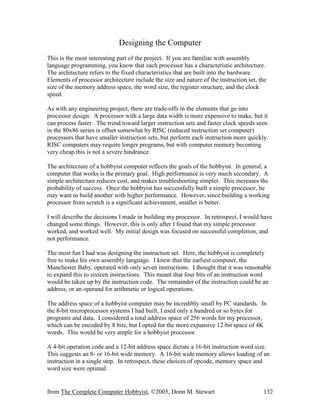
  • 5. from The Complete Computer Hobbyist, ©2005, Donn M. Stewart 136 Building the Data Path The data path of the computer is the ordered collection of registers that hold the data, the multiplexors that direct the flow of the data, and the ALU that operates on the data. The memory may also be considered part of the data path, although it is physically separated from the processor. Recall the simple machine cycle diagrammed in the previous chapter. We will start at this point and diagram the processor data path, using as an example the execution of the ADD instruction. This instruction is executed by the processor in several steps, each taking exactly one clock cycle to perform. We assume for now that the processor is running. The mechanism to start the processor will be discussed later. The ADD instruction that will be executed is part of a larger collection of instructions that reside in the computer memory. This collection of instructions is the program, and has been written and placed in the memory by the programmer. Exactly how this is done will also be discussed later. The computer memory is symbolized by a parallelogram. D CP Q QClock Register loads and displays results of previous cycle on each upward clock edge Computer circuits perform operations on the data displayed by the register
  • 6. from The Complete Computer Hobbyist, ©2005, Donn M. Stewart 137 The memory in our computer will be 16 bits wide, and at present will be shown with distinct data inputs and outputs. The memory address is specified a 12 bit input. We will assume for now that the memory acts like a large collection of registers in that a rising clock pulse edge at the Memory Write input will cause the data on the inputs to be loaded into the memory cell specified by the address. This data will then appear on the outputs. In the absence of a Memory Write pulse, the memory will simply display whatever data is present in the memory cell specified by the address input. The Memory Write signal will be derived from the processor control logic that will be described later. It is a single bit input. The first step in executing the ADD instruction is to get the instruction from memory. This is commonly called the instruction fetch step. Since the processor is running, it contains in the Program Counter register the address of the ADD instruction we want to fetch and execute. To get the ADD instruction out of memory, we simply send the output of the Program Counter register to the memory address inputs. After a few hundred nanoseconds, still well within the limits of one clock cycle, the desired instruction will appear on the memory data output lines. However, in order to execute the instruction we need to save it somewhere. We cannot simply keep it on the memory output lines, since we will need to get at least one of the ADD operands from the memory (the other operand is already in the accumulator register, left there by prior instructions). We will store the instruction in the Instruction Register. Memory Memory 16 16 Data in Data out 12 Address Memory Write
  • 7. from The Complete Computer Hobbyist, ©2005, Donn M. Stewart 138 All of the registers, like the memory, have Write inputs. To complete the instruction fetch cycle, we need to send an Instruction Register Write pulse to the Instruction Register. This pulse, like all the other register write signals, will come from the control logic, to be designed later. We now have diagrammed all the parts of that data path needed to complete the instruction fetch. After the instruction fetch, the computer will need to prepare itself to get the next instruction. Unless a jump instruction is being executed, the next instruction is in the memory cell immediately following the one just fetched. Therefore, we need to increase the value of the program counter by one. How can we do this? The answer is simple. We will have an ALU built into the processor, and it has nothing to do in the first part of the instruction fetch. Why not use it to add 1 to the Program Counter? The ALU can do this while the memory is getting the current instruction. By the time the current instruction is ready to be clocked into the instruction register, the incremented program counter is ready to be clocked into the PC register. Remember, we are using rising clock edge triggered registers, and the increased Program Counter value will not appear on the Program Counter Register outputs until the program counter write pulse arrives. This will happen at exactly the same time that the instruction register write pulse arrives at the instruction register. There will not be enough time for the new program counter value to confuse the system with another instruction, since the instruction register will be closed for inputs long before the new instruction appears on the memory data output. Until we send another IR write pulse during the fetch phase of the following instruction execution, the current ADD instruction will abide securely in the Instruction Register. Here is a diagram showing how we can use the ALU to increment the Program Counter. Remember the diagram of the ALU from previous chapters. Our ALU will process 12 bits and have a three-bit opcode. 16 16 Data in Data out 12 Address Program Counter Instruction Register Instruction Register Write Program Counter Write
  • 8. from The Complete Computer Hobbyist, ©2005, Donn M. Stewart 139 We do not use the carry in when the program counter is incremented. All we have to do is send the current Program Counter value to one input of the ALU, the 12-bit number 1 to the second (that is, binary 0000 0000 0001), and put the three bit ADD opcode on the ALU opcode inputs. After a short delay, the incremented Program Counter will appear at the ALU output and will be sent to the Program Counter inputs. It will wait there until the Program Counter Write pulse arrives, at which point the incremented program counter value will be loaded into the register, ready to fetch the next instruction. We have finished putting together the pathway for the instruction fetch and the program counter incrementation step. I will add to the diagram as we go through the rest of the ADD instruction execution. In order to make room in the diagram, I will not show the number of bits in each connection, nor the register write inputs from now on to reduce clutter. 12 12 12 1 Program Counter ADD Opcode Opcode Output Carry-in Carry-Out A input B input 3 12 12 12
  • 9. from The Complete Computer Hobbyist, ©2005, Donn M. Stewart 140 At the end of the instruction fetch/program counter incrementation cycle, the Program Counter Write and Instruction Register Write inputs receive clock pulses. The rising edge of these clock pulses locks the results of this cycle into these registers at the same instant, and then the next cycle begins. In the diagram, I show that the upper four bits of the IR holds the instruction opcode, and the lower 12 bits the instruction operand. These two parts of the IR are sent on different paths, as I will show soon. The next clock cycle is Instruction Interpretation. During this cycle, nothing happens in the data path. The instruction opcode (the upper 4 bits of the instruction register) is sent to the control logic. This opcode, along with the zero, minus, and carry condition flags, directs the control logic to set the control lines of the data path in such a way as to carry out the operation desired. In order to perform the ADD operation, the control logic will cause the data path to perform the following two steps, each taking one clock cycle. First, an operand stored in the memory will be fetched and placed in the Data register. Second, the Accumulator and Data register values will be sent to the ALU data inputs, and the three-bit ALU opcode for ADD will be sent to the ALU opcode input. At the end of this second step, on the rising edge of the next clock pulse, the ALU output will be stored in the Accumulator and the carry-out will be stored in a one-bit carry flip-flop. When the ADD operation is complete, the control logic will instruct the data path to begin another instruction fetch/program counter incrementation cycle, and execute the next instruction found in the computer memory. We need to expand our drawing of the data path to show the other registers and pathways involved in the ADD operation. First, we will add the components needed for the Data Register fetch step. PC Memory IR ALU 1 Opcode (bits 12-15) Operand (bits 0-11) Address in Data out Data in Add
  • 10. from The Complete Computer Hobbyist, ©2005, Donn M. Stewart 141 Notice that I added the Address Source Multiplexor to select the source of the memory address for the operand fetch. During the instruction fetch, the Program Counter held the address of the instruction. Now, the Instruction Register holds the address of the data to be placed in the Data Register for addition. Of course, the multiplexor input is selected by a signal from the control logic. At the end of this data fetch cycle, a register write pulse is sent by the control logic to the Data Register, but no write pulse is sent to the Instruction Register. This ensures that the Instruction Register will continue to hold the ADD instruction that was fetched earlier. During the final cycle of the ADD instruction, the contents of the Accumulator and Data registers are directed to the ALU inputs, along with the ADD opcode contained in the IR bits 12-14. After a short delay, the result of the addition will appear on the ALU output. This result will be clocked into the accumulator register by a write pulse at the end of the cycle. The carry-out bit will also be stored in a flip-flop. We will now add the Accumulator register and a few more elements to the data path diagram. PC Address source multiplexor Memory IR ALU 0 1 Add Data register Op- code Oper- and Addr Data out Data in PC = Program Counter IR = Instruction Register 1
  • 11. from The Complete Computer Hobbyist, ©2005, Donn M. Stewart 142 We need ALU source multiplexors to send the proper inputs to the ALU. In the Program Counter Incrementation step we sent the Program counter to the ALU A input, and the 12-bit value 1 to the ALU B input. In all the two-input arithmetic and logical instructions, such as ADD and OR, we will send the Accumulator to the ALU A input, and the Data Register to the ALU B input. We also need to add a multiplexor to select the ALU operation, either the stand-alone ADD operation for the PC incrementation step, or the ALU opcode contained in bits 12 to 14 of the Instruction Register. Notice how the ALU output is connected to both the Accumulator and Program Counter inputs. At the end of the last cycle of execution of the ADD instruction, the control logic sends a write pulse to the Accumulator and carry flip-flop. No write pulse is sent to the Program Counter, so it remains unchanged. After this final write pulse, the Accumulator will contain the result of the addition, and the Carry flip-flop will contain the carry-out bit. The data path diagrammed above is adequate for the instruction fetch/program counter incrementation cycle, and for all the arithmetic-logical operations except those using a carry-in (or borrow). To finish the data path for the arithmetic instructions that need a carry input, we add a path from the output of the Carry flip-flop to the ALU carry-in. Whether the carry-in is used or not depends on the ALU opcode, so there is no control line for this outside the ALU. PC Address source multiplexor Memory IR Accumulator ALU source multiplexors A B ALU ALU Op source multiplexor 0 0 1 Add 0 1 0 11 Data register 1 Op- code Oper- and Addr Data out Data in PC = Program Counter IR = Instruction Register Carry FF
  • 12. from The Complete Computer Hobbyist, ©2005, Donn M. Stewart 143 We now have a data path that will perform all eight of the arithmetic-logic instructions in our instruction set. A few more modifications will allow the other eight instructions to be performed. To perform the load/store instructions, connections between the accumulator and the memory are needed. There is only one type of store instruction, that is, store accumulator to memory (STM). However, there are two types of load instructions: load accumulator from memory (LDM), and load accumulator immediate (LDI). In the LDM (memory) load, the accumulator gets its input from the memory; the memory address is in the lower 12 bits of the instruction register. In the LDI (immediate) load, the value itself is in the instruction register. Therefore, we need an Accumulator Source Multiplexor to select the appropriate accumulator input: the ALU (from the arithmetic-logic instructions), the memory (LDM) or the instruction register (LDI). PC Address source multiplexor Memory IR Accumulator ALU source multiplexors A B ALU ALU Op source multiplexor 0 0 1 Add 0 1 0 11 Data register 1 Op- code Oper- and Addr Data out Data in PC = Program Counter IR = Instruction Register Carry FF
  • 13. from The Complete Computer Hobbyist, ©2005, Donn M. Stewart 144 This data path is able to execute the instruction fetch/program counter step, the arithmetic logical instruction steps, and the memory load/store instruction steps. The remaining instructions are the program flow, or jump instructions. These instructions operate by placing into the program counter a new value, either from the memory (indirect jump) or from the instruction register (direct jumps). Therefore, we need connections between the instruction register and the program counter, and the memory and the program counter. This means we need a PC source multiplexor to select the proper PC input. The conditional jumps in our limited instruction set are direct jumps, and whether they are executed or not depends the value of the carry flip-flop (jump on carry) or the value of the accumulator (jump on zero, or jump on minus). No extra connections are needed beyond those for the unconditional jumps. If the condition is met, the control logic will cause the (direct) jump to occur, and if not it will simply cause the data path to fetch the next instruction in memory, skipping the jump step. Carry FF PC Address source multiplexor Memory IR Accumulator source multiplexor Accumulator ALU source multiplexors A B ALU ALU Op source multiplexor 0 0 1 0 1 2 Add 0 1 0 11 Data register 1 Op- code Oper- and Addr Data out Data in PC = Program Counter IR = Instruction Register
  • 14. from The Complete Computer Hobbyist, ©2005, Donn M. Stewart 145 This completes the data path for the computer. There are some details that need to be added. Extra logic is needed in order to work with real computer memory that doesn't write like a register. This topic deserves its own section, which will follow. Also, some simple logic (11 two-input OR gates) is needed to derive the accumulator zero signal (the accumulator minus signal is simply the uppermost bit in the register). If you can understand the diagram above, you are well on your way to understanding a real computer at its most fundamental level. This data path can be built with standard IC components of the 74LS00 series. Specifically, there is an IC that has an 8-bit register in a 20-pin package, and two of these will do for the instruction register. Similarly, three 6-bit register IC's will make a 12-bit register. The 12-bit 4 input multiplexors can each be built of 6 dual one-bit multiplexor IC's, and the one-of-two multiplexors can be built from IC's that have four single-bit one- of-four multiplexors per chip. To make the zero logic, a 12-input OR gate can be used, made from 11 2-input OR gates on 3 IC's. One chip with the carry flip-flop is also needed. The total number of IC's needed for this data path is 34, and would cost about $17.00. Of course, the sockets and board increase the cost up to about $50.00. Carry FF PC PC source multiplexor Address source multiplexor Memory IR Accumulator source multiplexor Accumulator ALU source multiplexors A B ALU ALU Op source multiplexor 0 0 1 2 0 1 0 1 2 Add 0 1 0 11 Data register 1 Op- code Oper- and Addr Data out Data in PC = Program Counter IR = Instruction Register
  • 15. from The Complete Computer Hobbyist, ©2005, Donn M. Stewart 146 Real Computer Memory As mentioned in the previous section, real computer memory does not operate like a large collection of data registers. There are two main differences. First, the memory write process is more complicated, involving several signals that have to be created by the computer logic. Second, memory uses a bi-directional data path, called a data bus. The semiconductor RAM memory circuit I used in this computer is 4-bit by 1K static random access memory (SRAM), specifically the 2114 IC. Static RAM does not require refreshing every millisecond or so like the cheaper, faster dynamic random access memory (DRAM). It is important to build your hobbyist computer with SRAM, because in the troubleshooting phase of construction you will need to run it very slowly, one cycle at a time, in order to find out why it is not working. DRAM will not function in a single step cycle, unless it has its own clock circuit. An additional benefit of using SRAM is that you don't have to create the circuitry to perform the refresh cycles during normal operations. Now, one can buy DRAM with the refresh circuitry built in, called SDRAM. However, our computer uses so little RAM, that it makes sense just to use the old- fashioned 1K 2114 circuit. It is all the RAM you will ever need. The memory is written with the help of two inputs. The first is the chip select (CS) input, which must be made low (0 V) in order for the chip to function, either for input or output. The other input is the write input (WR). This input must be made low, and held low for a specified minimum time. During this time, the address and data on the memory inputs must be held steady. At the end of the required time span, the write input is made high (5V), and the data is locked into the memory. The key factor in the timing is that the memory write input must go high before the address or data inputs change, in order to ensure that the data is safely written. This presents a problem for the computer designer. He (or she) would like to write to the memory in a single cycle. However, at the end such a cycle, the address, data and memory write signals would all change at approximately the same time, putting the data in some peril. You might try to chance it, but there is a better way. The answer is to spread the memory write over two clock cycles. This gives us some additional clock edges with which to work. We can now ensure that the memory write goes high well before the data or address inputs have a chance to change. Here is the kind of timing we would like for a solid memory write:
  • 16. from The Complete Computer Hobbyist, ©2005, Donn M. Stewart 147 Each figure above represents the voltage level on the indicated memory inputs, or the clock. The memory write process proceeds this way. At the start of the first memory write clock cycle, A in the diagram, the processor puts the address of the memory location to be written on the address inputs of the memory. Simultaneously, the chip select memory input is made active (low) since this memory control input is derived directly from the address. One-half cycle later, on the downward edge of the clock in cycle A, the Memory Write (WR) is made active (low). At the beginning of the B cycle, the data is placed on the memory inputs, and on the downward edge of the clock in the B cycle, the WR input becomes inactive (high). At this point, the data is locked into the memory. At the end of the B cycle, on the upward clock edge of the next machine cycle, the address used during the memory write, and the derived CS input, are inactivated. The address, CS, data and WR are all active during the first half of the B cycle, which lasts 500 nanoseconds for a 1 MHz clock. This easily meets the minimum time requirement for writing the 2114 memory chip, which is about 200 ns. It is not hard to make a circuit that will provide the proper timing of the memory write input (WR). Here it is: Time Voltage A B System Clock Memory Write Chip Select Address for memory write Data for memory write Not ready Ready Not ready Not ready Not readyReady 0 CP D Q WR to memory System Clock Memory Write (from control logic)
  • 17. from The Complete Computer Hobbyist, ©2005, Donn M. Stewart 148 This is simply an edge-triggered flip-flop whose clock pulse input is the inverted system clock. The control logic Memory Write signal comes on (becomes one) at the beginning of the A machine cycle, in response to the program instruction STM. However, since the flip-flop has an inverted clock signal, it is not written into the flip-flop until the middle of the A cycle. That is, when the clock has a falling edge in the A cycle, the inverted clock input to the flip-flop will have a rising edge, and the Memory Write signal will be written into the flip-flop. It then appears on the output, and is inverted. This output is connected to the WR input on the memory chip (the WR signal to the memory chip is active when low.) When the WR memory input goes low, the memory begins to store the data that the processor has placed on its inputs. The Memory Write signal from the control logic goes to zero at the end of the machine cycle A, but since the flip-flop has an inverted clock input, the WR output is held low for another half-cycle, giving the memory the time it needs to finish storing the data. In the middle of the B cycle, the flip-flop sees a rising clock edge from the inverted clock input, and stores the Memory Write zero. The WR now goes to 1, and the memory write is finished. The timing diagram shows the requirements for writing a real semiconductor memory with the various control inputs. The other feature of memory, that makes it different from a register, is that it has bi-directional data input/output lines. These lines are controlled by a device called a three-state buffer, which I will now describe. Recall that a computer consists of large networks of automatic switches, each of which is either on (logical 1, or 5V) or off (logical 0, or 0V). But remember, that in order to be either 5 or 0 volts, an output has to be connected, through the logic gate circuit, to either the 5V or 0V (ground) power supply leads of the gate. What would be the state of an output that was connected to neither? That is, pretend you cut the output wire, and it is hanging in the air. Remember that the output voltage of a logic circuit is only part of an output. The other is the ability to pass current. So, if an output is 5V, it also needs to be able to pass some current to drive inputs of other gates to which it is connected. Similarly, if an output is 0V, it needs to be able to "sink" current, in order to operate the circuits it is tied to. The "cut wire" state is a third state, neither 1 nor 0, that is very useful in computer system design. The third state is also called "high impedance", because current will not be able to flow either into or out of an output that is in this state. The high impedance state can also be thought of as having a very high resistance. It is shortened to "Hi Z". Here is a simple switch diagram that shows a two-state and a three-state device. 1000 ohms Two-state output
  • 18. from The Complete Computer Hobbyist, ©2005, Donn M. Stewart 149 In the upper diagram, the switch can be open or closed. This type of switch is called a single-throw switch. If open, the output is connected through the resistor to ground, and will have a voltage of 0 with ability to sink some incoming current to ground through the resistor. When the switch is closed, the output will be 5V, with the ability to pass significant current to outside devices. The lower diagram shows a switch that can have three positions; closed to the 5V contact, open in the middle, or closed to the grounded contact. Such a switch is called a double-throw switch. Note that the circuit output is connected to the central pole of the switch. The middle position is the third state. It is just like a cut wire. The output, connected to the central pole of the switch, will not be able to conduct any current anywhere with the switch in the middle position and its voltage will be undefined. This is characteristic of the third, or high-impedance state. Having a three-state logic device output allows us to take a huge short cut when we assemble a true computer system. It allows us to use a collection of wires to pass data in two different directions. A collection of parallel wires is called a bus, and when it can pass data in two directions it is called a bi-directional bus. The bi-directional bus allows us to connect many separate devices that have three-state outputs to the same set of wires, and then use logic to select which devices will communicate to each other. The other unselected devices will remain in the third state, and will be invisible to the active circuits. They will not interfere with the data communications between the active devices. We are bringing this up here, because computer memory is such a device, with three-state data outputs. When the memory write signal is given to a selected memory chip, the outputs behave as data inputs, in order to write data in the memory. When the memory write signal is inactive, the outputs behave as outputs, sending data onto the bus. When the chip is not selected, the outputs are in the third, high-impedance state, and the chip is invisible to other devices on the bus, such as input or output ports. It is convenient to think of the memory data lines as input/output lines, because they can change direction. It is a simple matter to make a bi-directional bus using three-state logical devices. The two most commonly used are the three-state buffer, and three-state inverting buffer. Switch contact swings both ways Three-state output
  • 19. from The Complete Computer Hobbyist, ©2005, Donn M. Stewart 150 The control input is a signal that enables the gate to pass data when it is on (1). The control input is sometimes called an enable input. Here is how to make a bi-directional buffer out of two three-state buffers and an inverter. When control is 1, the data flows from A to B, and when it is 0, from B to A. In other words, when control is 1, A is the input and B is the output, and when control is 0, B is the input and A is the output. Thus A and B are input/outputs. Inclusion of another control can allow the bi-directional buffer to go to the Hi Z state. This type of circuit is used inside memory circuits to control the input/output lines Input Output Input Output Control input Control input In Control Out 0 0 Hi Z 1 0 Hi Z 0 1 0 1 1 1 In Control Out 0 0 Hi Z 1 0 Hi Z 0 1 1 1 1 0 B A Control A Control B Select Control Direction 1 0 B to A 1 1 A to B 0 0 Hi Z 0 1 Hi Z Select
  • 20. from The Complete Computer Hobbyist, ©2005, Donn M. Stewart 151 In the data path defined in the previous section, we are faced with the problem of how to connect a register, with separate inputs and outputs, to a memory chip with bi-directional three-state input/outputs. First of all, the problem really only occurs during the memory write cycle, because otherwise the memory is either putting out data (if selected) or is in the high impedance state (if not selected). If the memory input/outputs are directly connected to register inputs, both of these conditions are tolerable. However, the register outputs cannot be connected directly to the memory input/outputs, because when the memory is in the output condition, you will have memory outputs connected to register outputs, which is not tolerable. We will use a three-state buffer to prevent the register outputs from being connected to the memory input/outputs as long as the memory is in the output condition. The circuit is simple: The three-state buffer protects the memory outputs from colliding with the register outputs when the memory is in the output mode. When the memory goes into the input mode, and the memory input/outputs become inputs, then the Data out control signal comes on, and the three-state buffer becomes an output. In the timing diagram shown earlier, this takes place at the beginning of the B machine cycle. Note that using a three- state buffer to make a bi-directional data bus doesn't bother the register at all; its inputs are always connected to outputs, regardless of whether the memory is in input or output mode. Here is a diagram of the data path with the three-state data out buffer included. Now, the memory input/outputs are connected to a bi-directional data bus. CP D Q Bi-directional data bus Memory Register Register write pulse Three-state buffer Data out to memory
  • 21. from The Complete Computer Hobbyist, ©2005, Donn M. Stewart 152 The only devices capable of putting an output on the data bus are the accumulator (during a memory write) and the memory (most of the rest of the time). The other devices (multiplexors and registers) are always inputs. Inputs don't interfere with bus traffic. We can put other devices on the bus, such as input/output ports. Any device that places data onto the bus, like an input port when active, will need to have three-state outputs. Then, we can read from or write to ports as if they were memory locations, using memory load or store instructions. The only difference is that the numbers we write will affect the devices attached to the port. This is how we will connect our computer to the outside world. It is the address in the instruction that will activate either the memory, or the ports. As long as the devices that place data onto the bus have three-state outputs, and as long as we avoid colliding outputs by proper logic, there is no limit to the number of devices that can use the bus. Carry FF PC PC source multiplexor Address source multiplexor Memory IR Accumulator source multiplexor Accumulator ALU source multiplexors A B ALU ALU Op source multiplexor 0 0 1 2 0 1 0 1 2 Add 0 1 0 11 Data register 1 Op- code Oper- and Addr Data in or out PC = Program Counter IR = Instruction Register Three-State Data out buffer Bidirectional Data Bus
  • 22. from The Complete Computer Hobbyist, ©2005, Donn M. Stewart 153 The Machine within the Machine--Control Logic The data path described in the previous chapter is the tool kit of the computer. The registers and multiplexors, together with the ALU and the memory, have the power to perform all the operations of the instruction set we designed earlier. However, it is the control logic that really runs the computer. It coordinates and controls all the data path elements. The control logic takes as its input the instruction operation code, and generates a sequence of outputs that causes the data path to manipulate data or alter the flow of the computer program. For each instruction, the control logic defines a series of steps. With each step, the control logic generates specific outputs. These outputs are fed to the data path multiplexor and register write inputs. Each step of the sequence is designed to be performed in a single clock cycle. If we want to perform a task that does not fit into one clock cycle, we need to break it up into sub-steps. The control logic keeps track of these steps by assigning a unique number to each one, called the state. The state is kept in a register in the control logic circuitry. A device that uses a finite number of states in specified sequences to control a process is called a finite state machine. The machine works as follows. The cycle starts at some initial entry state, which we will assign the number 0. This value is placed into the state register. The control logic then looks at the state register and the current instruction opcode. Using standard AND/OR logic gates, it then creates two outputs. One output is the pattern of 1's and 0's that is sent to the data path elements (multiplexors and registers) to perform data and program flow manipulations. The other output is the next state. At the end of the clock cycle, the next state is written into the state register. At this point, the next state becomes the current state for the next cycle. Control Logic State register Clock Control output to Data Path Next State output to state register Current State input from state register Instruction Opcode input from instruction register
  • 23. from The Complete Computer Hobbyist, ©2005, Donn M. Stewart 154 The state register is written every clock cycle, and therefore the computer clock is directly connected to its write input. Different instructions can use the same states. For example, all instructions will start with state 0, which is the instruction fetch/program counter incrementation step. This will always be followed by state 1, which is the instruction interpretation step. If the processor is executing an arithmetic/logic instruction that has two operands, it will use a data fetch step. All arithmetic/logic instructions can use the same state for the data fetch step. The arithmetic/logical instructions that write the carry flip-flop can all use the same state, and the ones that do not can all use the same state. When the final state of a sequence is finished, the next state logic will give a 0 as its output, and a new sequence will start. Once the sequence of states is built into the control logic, the cycle operates endlessly. How many states are required? Our instruction set has 16 operations, and each operation will need from 2 to 4 steps (or states) to operate. However, many states are shared by several operations, and this reduces the total number of states required. In fact, our computer can be built with a control logic that uses only 11 states (0 to 10). Modern complex instruction set processors, such as the Pentium, need hundreds of states. By looking at the data path diagram, and thinking about what needs to happen in order for an instruction to be carried out, we can make a list of the states that will do everything our instruction set needs to do. Here are the states for this processor. The numbers we assign are somewhat arbitrary, although it is important to make state 0 the first step. This allows us to use a simple circuit to start the computer. State Action 0 Instruction fetch/program counter incrementation 1 Instruction interpretation 2 Data fetch 3 Arithmetic instruction, includes carry write 4 Logic instruction, no carry write 5 Load accumulator immediate (value in current instruction) 6 Load accumulator from memory 7 Store accumulator to memory, first step 8 Store accumulator to memory, second step 9 Jump immediate 10 Jump indirect By referring to these states, we can now associate each instruction in our instruction set with the sequence of states needed to carry it out. We have already shown how the sequence of states 0,1,2,3 will perform the ADD operation. Here is the complete instruction set with the corresponding state sequences.
  • 24. from The Complete Computer Hobbyist, ©2005, Donn M. Stewart 155 Instruction Opcode Condition Opcode Mnemonic State sequence 0000 ADD 0,1,2,3 0001 ADC 0,1,2,3 0010 SUB 0,1,2,3 0011 SBC 0,1,2,3 0100 AND 0,1,2,4 0101 OR 0,1,2,4 0110 XOR 0,1,2,4 0111 NOT 0,1,4 1000 LDI 0,1,5 1001 LDM 0,1,6 1010 STM 0,1,7,8 1011 JMP 0,1,9 1100 JPI 0,1,10 1101 Z = 0 (not zero) JPZ 0,1 1101 Z = 1 (zero) JPZ 0,1,9 1110 M = 0 (not minus) JPM 0,1 1110 M = 1 (minus) JPM 0,1,9 1111 C = 0 (not carry) JPC 0,1 1111 C = 1 (carry) JPC 0,1,9 Notice that the arithmetic operations all use the same sequence of states. The difference between addition and subtraction, and the use of the carry-in, depends on the three-bit ALU opcode that is imbedded in the instruction opcode, so we do not need separate states for each. Similarly, the logical operations share the same sequence, the difference being that state 5 does not write the carry-out to the carry flip-flop. The NOT operation, which does not have a second operand, skips the data fetch state. The conditional jump instructions use the same state sequence as the unconditional direct jump when the corresponding condition is met. If the condition is not met, the direct jump state is simply omitted and the instruction performs no operation at all. Since each state is one clock cycle long, we can tell how long each instruction will take to execute. If we assume a clock rate of one megahertz, then the processor should be able to execute an addition (or any other 4-state instruction) in 4 microseconds. We will create the control logic so that the control output depends only on the current state. There are other ways to do this, such as making the control output for the conditional jumps depend on the condition, but I think this way is simpler. I will now show a table of the control outputs that correspond to each state. There is one control output for each data path control input. Note that a three-input multiplexor needs two control inputs, for the low order and high order bits (bits 0 and 1). Refer to the data path diagram for the elements that use control inputs.
  • 25. from The Complete Computer Hobbyist, ©2005, Donn M. Stewart 156 Control input State 0 1 2 3 4 5 6 7 8 9 10 Program Counter Multiplexor Low 1 X X X X X X X X 0 0 Program Counter Multiplexor High 0 X X X X X X X X 0 1 Program Counter Write 1 0 0 0 0 0 0 0 0 1 1 Memory Address Multiplexor 1 X 0 X X X 0 0 0 X 0 Memory Write 0 0 0 0 0 0 0 1 0 0 0 Memory Data Out 0 0 0 0 0 0 0 0 1 0 0 Instruction Register Write 1 0 0 0 0 0 0 0 0 0 0 Accumulator Multiplexor Low X X X 0 0 1 0 X X X X Accumulator Multiplexor High X X X 0 0 0 1 X X X X Accumulator Write 0 0 0 1 1 1 1 0 0 0 0 Data Register Write 0 0 1 0 0 0 0 0 0 0 0 ALU A Multiplexor 1 X X 0 0 X X X X X X ALU B Multiplexor 1 X X 0 0 X X X X X X ALU Operation Multiplexor 1 X X 0 0 X X X X X X Carry flip-flop Write 0 0 0 1 0 0 0 0 0 0 0 X = don't care Notice that we don't care what the multiplexor control inputs are if we are not going to write the registers (or memory) whose input is supplied by that multiplexor. The "don't cares" allow us to design the logic more efficiently. Also, note that some of the control lines behave identically across all states. It is easy to see that the ALU A and B multiplexor control lines, and the ALU operation multiplexor control line could all be replaced by a single control line. Other control lines might also be consolidated, such as the program counter multiplexor low and the instruction register write. However, I felt that extensive consolidation of control lines might be confusing when it came to troubleshooting the processor, so I only consolidated the ALU multiplexor lines. It is more important to minimize the number of states needed. In the control design above, no two states can be consolidated. In order to make a circuit that will "map" one state to one control output we have two main options. The option used by most processor manufacturers is to use microcode. The microcode technique uses a read-only memory to hold the control output configurations, in the form of binary numbers. The control output for each state in the above table could be considered as a 15-bit binary number. We can store the control output configuration for each state in such a way that Carry Flip-Flop Write is in the rightmost (low) bit, and the Program Counter Multiplexor Low is in the leftmost (high) bit. If we replace the don't cares with 0, then the control line output for state 0 would be the binary number 101 1001 0000 1110. The control line output simply becomes a 15-bit wide memory with 11 locations, one for each state.
  • 26. from The Complete Computer Hobbyist, ©2005, Donn M. Stewart 157 For the hobbyist, this arrangement is attractive because the control output function can be changed without rewiring circuits. However, it requires the programming of ROM, and this requires extra equipment. But it is likely that you will need a PROM programmer anyway, so it is reasonable to consider this. The other way to make a circuit that "maps" a state onto a control output is to use a decoder, together with AND-OR logic. In this method, the control output for each state is hard-wired into the board. If you like to wire things up, this is the way to go, and this is the way I did it. Without showing the whole circuit, here is an example of how the states might be decoded into the corresponding control outputs Program Counter Multiplexor Low Program Counter Multiplexor High Program Counter Write Memory Address Multiplexor Memory Write Memory Data Out Instruction Register Write Accumulator Multiplexor Low Accumulator Multiplexor High Accumulator Write Data Register Write ALU A Multiplexor ALU B Multiplexor ALU Operation Multiplexor Carry flip-flop Write The 4-bit state value is placed on the decoder inputs, and the corresponding output becomes 1. The other outputs are 0. The Program Counter Write and Accumulator Write control lines are on in several different states, so multiple input OR gates are required to provide these outputs. The other control lines are connected directly to only one state output. If you compare this circuit with the table on the previous page, replacing the X 0 21 3 54 6 7 98 10 Four-to-sixteen state decoder 4-bit State input (from state register)
  • 27. from The Complete Computer Hobbyist, ©2005, Donn M. Stewart 158 don't cares with zeros, you can see that this simple circuit faithfully provides the appropriate control outputs. This circuit can be built with one 4-to-16 decoder and 6 two- input OR gates, a total of 3 IC's. The control logic is half done. The other function of the control logic is to provide the sequence of states for each instruction. We call this the next-state function. The next-state function circuitry takes as its inputs the current state, the current instruction, and the conditions (zero, minus and carry). From these inputs, the next state is determined. The next-state function circuit is more difficult to design than the control output circuit. This is because it has a much more complex input. If we count each bit of the current state, current instruction and conditions, there are 4 + 4 + 3 = 11 bits of input, instead of the 4 bits of input to the control output circuit. Eleven bits can encode over 2,000 different combinations instead of the 16 handled by the simple decoder-based circuit we used for the control outputs. Of course, not all these combinations are used, and although there are 16 instructions there are only 11 states. Also, some instructions use the same sequence of states, and most don't care about the condition flags. Nevertheless, the next state function design requires some thought. As with the control outputs, a microcode contained in a programmable ROM could also provide the next state function. The current instruction, current state and condition flags could be used to form an address, and the output would be the next state. In fact, the control output and next state function could be combined into a single PROM, with an 11-bit address and 19-bit output (4 bits for the next state, 15 bits for the control outputs). A more elegant way to encode the next state function is to use the technique of AND-OR arrayed logic. This type of logic is able to encode any function that maps an input to a unique output. With the inclusion of inverters, arrayed logic has the power to perform all the functions of the digital computer. In fact, programmable array logic IC's can be used to create entire microprocessors. We already saw an example of AND-OR array logic in the chapter about building the ALU. In our case, we will first diagram the next state function as an AND-OR array, and then show how to build it. Keep in mind that the AND-OR array diagram is not a circuit diagram, but only a plan that will allow us to build the actual array. The diagram consists of two parts. The upper part shows how the inputs are connected to multiple input AND gates. The lower part shows how the outputs of these AND gates are connected to multiple input OR gates. The OR gate outputs are the outputs of the circuit, the next state value. The first step in creating the next state operation is to map it out in a table. This will show us what we need to do when it comes to building the circuit. We will list all possible combinations of current state, current operation and condition flags, and the
  • 28. from The Complete Computer Hobbyist, ©2005, Donn M. Stewart 159 corresponding next state. First, we will make the table with decimal values for the states, using the mnemonics for the operations. Current state Operations Condition Next state 0 Don't care Don't care 1 1 ADD, ADC, SUB, SBC, AND, OR, XOR Don't care 2 1 NOT Don't care 4 1 LDI Don't care 5 1 LDM Don't care 6 1 STM Don't care 7 1 JMP Don't care 9 1 Conditional jumps Condition met 9 1 Conditional jumps Condition not met 0 1 JPI Don't care 10 2 ADD, ADC, SUB, SBC Don't care 3 2 AND, OR, XOR Don't care 4 3 Don't care Don't care 0 4 Don't care Don't care 0 5 Don't care Don't care 0 6 Don't care Don't care 0 7 Don't care Don't care 8 8 Don't care Don't care 0 9 Don't care Don't care 0 10 Don't care Don't care 0 The "don't care" entries show which states are always followed by the corresponding next state, regardless of the operation or condition. The above table must be made into a circuit. In order to do this, we will need to look at the binary representations of the current state, operation and condition, and figure out how combine them to make a binary representation of the next state using AND-OR array logic. It is convenient to think backward in making the AND-OR array. In other words, we look at each bit of the next state, and ask what kind of AND-OR operation is needed to get it from the corresponding current state, operation and condition as listed in the table above. Let us label the next state bits NS0 to NS3, (from low bit to high bit.) We will create operations that will cause the next state bit in question to become 1 when the input calls for it. We do not have to intentionally create an operation that will make the bit 0, because by default the bit will be 0 if it is not 1 (such is the elegance of the binary computer).
  • 29. from The Complete Computer Hobbyist, ©2005, Donn M. Stewart 160 Let's start with NS0. It will be 1 when the next state is 1, 3, 5, 7, or 9. If we look at the table above, we can see that NS0 will be 1 when: Current state Operations Condition 0 Don't care Don't care 1 LDI Don't care 1 STM Don't care 1 JMP Don't care 1 Conditional jumps Condition met 2 ADD, ADC, SUB, SBC Don't care Now let's re-write this table using the binary equivalents, including the conditions. Current state Operation Z M C 0 0 0 0 X X X X X X X 0 0 0 1 1 0 0 0 X X X 0 0 0 1 1 0 0 1 X X X 0 0 0 1 1 0 1 1 X X X 0 0 0 1 1 1 0 1 1 X X 0 0 0 1 1 1 1 0 X 1 X 0 0 0 1 1 1 1 1 X X 1 0 0 1 0 0 0 0 0 X X X 0 0 1 0 0 0 0 1 X X X 0 0 1 0 0 0 1 0 X X X 0 0 1 0 0 0 1 1 X X X The X's stand for "don't care". This table can be simplified a little. Some of the bits can be replaced with "don't care" (X) if the two rows are otherwise identical, and the bit in question is a 1 in one row, and a 0 in the other. For example, rows 2 and 3 can be replaced by a single row in which the low order bit of the operation is a "don't care". Similarly, the last four rows can be combined into a single row with two don't cares in the lower 2 opcode bits. Here is the simplified table: Current state Operation Z M C 0 0 0 0 X X X X X X X 0 0 0 1 1 0 0 X X X X 0 0 0 1 1 0 1 1 X X X 0 0 0 1 1 1 0 1 1 X X 0 0 0 1 1 1 1 0 X 1 X 0 0 0 1 1 1 1 1 X X 1 0 0 1 0 0 0 X X X X X This is the minimal table for the next state zero bit (NS0). Now, we are ready to draw the AND-OR array diagram for this table. All the 11 input bits (4 current state, 4 operation bits, and the 3 condition bits) are used in at least one row, so we will have 11 horizontal lines in the array diagram. We will include 11 inverted inputs to be used when an input bit is 0. There are 7 rows in the above table, each representing one multiple-input AND operation, so there will be 7 vertical lines in the array diagram. The 7 vertical lines will be connected in the lower part of the diagram by a horizontal line that represents the
  • 30. from The Complete Computer Hobbyist, ©2005, Donn M. Stewart 161 ORing together of the AND operation outputs. The output of this OR operation is the NS0 bit. The diagram looks complicated, but the circuit that it represents can be made with surprisingly few components. This is because several of the AND combinations (vertical lines) share patterns. For example, all 7 AND combinations use ((NOT Current State 3) AND (NOT Current State 2)). This can be handled by one two-input AND gate. Depending on how carefully you look for combinations to re-use, this circuit can be built with about 24 two-input AND gates, 8 inverters, and 6 two-input OR gates (the inverters on the condition lines are shown, but not used). This represents 10 14-pin IC's, which is not a difficult job. However, a clever reader may note that the AND patterns of the states and operations are the same as that for a decoder. If we use the outputs from the state decoder used previously in the control output circuit we can save some AND gates. Here is the same AND-OR array diagram using the decoded state lines. I only show the state lines actually used in the array; the others will have no connection in the next-state bit 0 array diagram. Current state 3 Current state 2 Current state 1 Current state 0 Operation 3 Operation 2 Operation 1 Operation 0 Z M C Next State 0
  • 31. from The Complete Computer Hobbyist, ©2005, Donn M. Stewart 162 This version uses only 18 AND gates, 4 inverters and 6 OR gates. Since the state decoder is already part of the logic circuitry, this is a reasonable way to proceed. Here are the binary tables for the other next state output bits. NS1: (when next state = 2,3,6,7,10) Current state Operation Z M C 0 0 0 1 0 0 X X X X X 0 0 0 1 0 1 0 X X X X 0 0 1 0 0 0 X X X X X 0 0 0 1 1 0 0 1 X X X 0 0 0 1 1 0 1 0 X X X 0 0 0 1 1 1 0 0 X X X NS2: (when next state = 4,5,6,7) Current state Operation Z M C 0 0 1 0 0 1 0 X X X X 0 0 1 0 0 1 1 0 X X X 0 0 0 1 0 1 1 1 X X X 0 0 0 1 1 0 0 X X X X Operation 3 Operation 2 Operation 1 Operation 0 Z M C Next State 0 State = 0 State = 1 State = 2
  • 32. from The Complete Computer Hobbyist, ©2005, Donn M. Stewart 163 NS3 (when next state = 8,9,10) Current state Operation Z M C 0 1 1 1 X X X X X X X 0 0 0 1 1 0 1 1 X X X 0 0 0 1 1 1 0 1 1 X X 0 0 0 1 1 1 1 0 X 1 X 0 0 0 1 1 1 1 1 X X 1 0 0 0 1 1 1 0 0 X X X Here is the AND-OR array diagram for the entire next-state operation. Operation 3 Operation 2 Operation 1 Operation 0 Z M C Next State 0 State = 0 State = 1 State = 7 State = 2 Next State 1 Next State 2 Next State 3
  • 33. from The Complete Computer Hobbyist, ©2005, Donn M. Stewart 164 The diagram suggests a lot of AND gates will be needed. But wait--more simplification is possible. First, we can eliminate the unused inverted condition flag lines. More importantly, we notice that some of the vertical lines have exactly the same patterns of dots. This means one or more can be eliminated, and the output of a single AND operation sent to the OR gates that received the output of the AND operations we eliminate. You can also see this if you look carefully at the next state bit tables. For example, the second row in the NS0 table is exactly the same as the fourth row in the NS2 table. We can use a single vertical line representing this particular AND operation, and connect the output to the OR gate inputs for the NS0 and NS2 bits. In all, there are 7 AND operations that can be shared by different NS output bits. Here is the final, simplified next state AND-OR array diagram. The circuit described by this diagram can be built with 34 two-input AND gates, four inverters, and 20 2-input OR gates. These gates can be purchased in 14-pin IC's with 4 logic gates or 6 inverters each. Fewer IC's can be used if one purchases the available three or four input AND and OR gates. The entire control logic described in this chapter can be built of 15 next-state IC's, plus three IC's for the control logic, plus one 4-bit register IC, or 19 IC's total. The cost would be about $8.00 for these chips, but again you have to buy the board and sockets for a lot more money. Operation 3 Operation 2 Operation 1 Operation 0 Z M C Next State 0 State = 0 State = 1 State = 7 State = 2 Next State 1 Next State 2 Next State 3