A learning based transportation oriented simulation system

Transportation Research Part B 38 (2004) 613–633
www.elsevier.com/locate/trb

A learning-based transportation oriented simulation system
Theo A. Arentze, Harry J.P. Timmermans *

Urban Planning Group/EIRASS, Eindhoven University of Technology, P.O. Box 513, 5600 MB,
Eindhoven, The Netherlands
Received 27 March 2000; received in revised form 17 August 2002; accepted 11 October 2002

Abstract

This paper describes the conceptual development, operatonalization and empirical testing of Albatross: A
Learning-based Transportation Oriented Simulation System. This activity-based model of activity-travel
behavior is derived from theories of choice heuristics that consumers apply when making decisions in
complex environments. The model, one of the most comprehensive of its kind, predicts which activities are
conducted when, where, for how long, with whom, and the transport mode involved. In addition, various
situational, temporal, spatial, spatial-temporal and institutional constraints are incorporated in the model.
The decision tree is proposed as a formalism to represent an exhaustive set of mutually exclusive rules for
each decision step in the model. A CHAID decision tree induction method is used to derive decision trees
from activity diary data. The case study conducted to develop and test the model indicates that perfor-
mance of the model is very satisfactory. We conclude therefore that the methodology proposed in this
article is useful to develop computational process models of activity-travel choice behavior.
Ó 2003 Elsevier Ltd. All rights reserved.

Keywords: Activity-based modeling; Computational process modeling; Decision tree induction; Reinforcement learning

1. Introduction

The activity-based approach in travel demand modeling implies a shift in focus from trips to
activities assuming that most travel is not an end in itself but a means to bridge activities that are
separated in time and space. The aim of the models is to explain and predict for a given time frame
and in an integrated fashion, which activities individuals conduct, where, when, for how long,
sometimes with whom, and the transport mode used. The choice of an activity-travel pattern that

*
Corresponding author. Tel.: +31-40-247-3315; fax: +31-40-247-5882.
E-mail address: h.j.p.timmermans@bwk.tue.nl (H.J.P. Timmermans).

0191-2615/$ - see front matter Ó 2003 Elsevier Ltd. All rights reserved.
doi:10.1016/j.trb.2002.10.001

614 T.A. Arentze, H.J.P. Timmermans / Transportation Research Part B 38 (2004) 613–633

meets space–time, institutional and household constraints and satisfies as much as possible
preferences of the individual, is an inherently complex cognitive task. Acknowledging this com-
plexity, several authors have stressed the importance of understanding the decision making
processes that underlie activity patterns and proposed computational process models that are
consistent with cognitive theories of problem solving, decision making and learning.
The production system is the most influential model of higher-order cognitive processes in
cognitive sciences, since it was introduced by Newell and Simon in the early seventies (1972). A
production system consists of a set of condition–action rules, called productions, representing
long-term memory of the individual and a set of currently active facts or beliefs about a given
problem in short-term memory. The systems describe problem solving as a cyclic process of
matching productions with items in short-term memory and adding the action of an executed
production to short-term memory. Because added actions may trigger other productions, the
process is repeated until all productions have been tried. The sequence of actions represents steps
and the final state of short-term memory the outcome of a problem solving process. Think out
loud protocols and many experimental findings in the area of memory, learning, and problem
solving have been successfully reproduced in production systems (e.g., Anderson, 1983).
As argued by G€rling (1998), this cognitive theory points at forms of imperfect choice behavior
a
not covered by current utility-maximization models based on economic theory. The implications
are particularly relevant for activity-based models which consider choices on many facets in in-
teraction. The number of possible activity-travel patterns is the product of all feasible activity
sequences and activity profiles. As described by production systems, individuals search a solution
space only partially based on heuristics that often yield satisfactory outcomes, but which are not
necessarily optimal. The heuristics used determine the sequence in which decisions are made and
the choice alternatives and attributes evaluated, and, hence, have impact on outcomes of the
process. It is the central argument for computational process models that, even if one is interested
in outcomes only, the process by which outcomes are generated needs to be represented in
activity-based models. G€rling et al. (1994) comprehensively discuss the theoretical underpinning
a
of these models.
Despite the well-established status of computational process theory, existing attempts to de-
velop computational process models (CPM) are limited. To review work in this field, we make a
distinction between a weak and strong definition of CPM. A weak CPM applies a heuristic in the
form of some sequential or partially sequential decision making process, but still assumes utility-
maximization or some other form of unbounded rationality at the level of individual decision
steps. Regardless whether or not reference is made to theories of heuristic search, several oper-
ational activity-based models exist that meet the weak definition. Examples are PCATS (Ki-
tamura and Fujii, 1998), the model system proposed by Bhat (Bhat, 1999), STARCHILD (Recker
et al., 1986a,b) and SMASH (Ettema et al., 1993). These models differ in various respects, but
have in common that logit models or other forms of algebraic equations are used to predict single-
facet choices.
Computational process models that fit the strong definition use a production system or some
other rule-based formalism also at the level of individual choice facets. Models that meet this
definition are scarce. The best example is SCHEDULER, developed by G€rling et al. (1989).
a
These authors developed a conceptual framework for understanding the process by which indi-
viduals organize their activities (G€rling et al., 1989, 1992a,b). This framework has been applied
a

T.A. Arentze, H.J.P. Timmermans / Transportation Research Part B 38 (2004) 613–633 615

to study the possible impact of the introduction of tele-commuting on the activity patterns of
commuters (G€rling et al., 1994). Only recently, parts of this conceptual model were elaborated
a
and subject of experimental investigation (G€rling et al., 1997, 1998, 1999). Strongly based on this
a
model is GISICAS which uses search heuristics in combination with GIS to generate feasible
schedules (Kwan, 1997). Another attempt to formulate a rule-based model has been reported
in Vause (1997), but apparently this work has been discontinued.
This brief summary of the state-of-the-art of computational process models indicates that, to
the best of our knowledge, fully operational rule-based models have not been developed to
date. Arguably, the lack of a method of empirically deriving rules of a production system has
hampered progress in this field (Golledge et al., 1994). Furthermore, the verification of
completeness and consistency of production systems presents a problem (Vause, 1997). While
being consistent with assumptions of (strong) computational process models, the decision tree
provides an alternative formalism that has favorable properties in both respects. Methods to
induce decision trees from data are available from work in statistics and artificial intelligence.
These methods develop a tree by recursively splitting a sample of observations into increas-
ingly homogeneous groups in terms of a given response variable. Decision trees induced in this
way describe the data and, at the same time, meet requirements of completeness and consis-
tency.
In this article, we propose a fully operational computational process model based on the de-
cision tree formalism. Albatross, as the model is called, was developed for the Dutch Ministry of
Transportation, Public Works and Water Management, to explore possibilities of a rule-based
approach and develop a travel demand model for policies impact analysis. This article describes
the conceptual underpinning, operationalization and validation testing of the model. The first
section discusses central concepts followed by a description of the proposed approach. An ac-
tivity-travel diary survey was conducted to collect data for deriving and testing the model. The
sections that follow describe the results of the empirical study. The paper concludes with dis-
cussing the major conclusions and avenues for future research.

2. Conceptual considerations

Consistent with the activity-based approach, we postulate that observed transportation pat-
terns are the result of a complex decision-making process by which individuals try to achieve
particular goals in the pursuit of their activities within the spatial-temporal and institutional
constraints set by the environment. This section describes the concepts and assumptions under-
lying the Albatross model regarding decision making and choice behavior.

2.1. Decision making

The organization of activities and related travel takes place in the context of an ever-changing
physical environment, an uncertain transportation environment and multi-day variations in
planned and unplanned activities that need to be completed. It is postulated that activity par-
ticipation, allocation and implementation fundamentally take place at the level of the household.
It is at that level that particular activities need to be performed, and it is also the household that is


involved in the decision which activities to conduct. The actual generation and execution of
activity calendars, programs and schedules covers a multitude of time frames.
First, long-term decisions made at the household level strongly influence the generation and
composition of activity calendars. Decisions regarding marital status, number of children, and
the like, are irreversible or require years to change, and hence have a strong impact on the
number and kinds of activities that need to be performed and the constraints that households
face. These variables also influence the discretionary activities, reflecting an assumed rela-
tionship between socio-demographic variables and lifestyle. Other long-term decisions, such as
choice of residence, choice of work and workplace, and purchase of transport modes can in
principle be changed in the short run, but in general represent the kind of choices that are not
changed immediately. Hence, these decisions exert a strong influence on possible activity
patterns as the location of the residence and workplace vis--vis the transportation sys-
a
tem represent the main locations of an activity pattern and are the cornerstones of deci-
sions.
Thus, these long-term decisions will influence household activity participation decisions. It is up
to household members to allocate these activities to household members. The actual allocation
will reflect task allocation mechanisms within the household, which will depend on gender-specific
roles, and time pressures. The task allocation and related allocation of activities involves the set of
activities that needs to be completed within a particular time horizon. It results in an individual
activity program that is derived from the household activity calendar. We postulate that this
process of program generation depends on the nature of the activities (mandatory versus dis-
cretionary), the urgency of completing a particular activity on a specific day as a function of the
history of the activity scheduling and implementation process, and the desire to meet particular
activity and time-related objectives.
Once the individual activity program has been generated, the next step is to schedule these
activities, which involves a set of interrelated decisions including the choice of location where to
conduct a particular activity, the transport mode involved, the choice of other persons with whom
to conduct the activities, the actual scheduling of activities contained in the activity program,
and the choice of travel linkages which connect the activities in time and space.
These activity scheduling decisions thus transform an individualÕs activity program into an
activity pattern, which is an ordered sequence of activities and related travel at particular loca-
tions, with particular start times and duration, with particular transport modes and perhaps
coordinated with the activity patterns of other individuals. In this context, travel decisions rep-
resent a sub-decision. Transport mode decisions dictate the action space within which individuals
can choose locations to conduct their activities. The organization of trips into chains allows in-
dividuals to conduct more activities within a specific time frame.
The actual process of scheduling activities is conceptualized as a process in which an individual
attempts to realize particular goals, given a variety of constraints that limit the number of feasible
activity patterns. Several types of constraints can be identified:

(1) Situational constraints impose that a person, transport mode and other schedule resources
cannot be at different locations at the same time.
(2) Institutional constraints, such as opening hours, influence the earliest and latest possible times
to implement a particular activity.


(3) Household constraints, such as bringing children to school, dictate when particular activities
need to be performed and others cannot be performed.
(4) Spatial constraints also have an impact in the sense that either particular activities cannot be
performed at particular locations, or individuals have incomplete or incorrect information
about the opportunities that particular locations may offer.
(5) Time constraints limit the number of feasible activity patterns in the sense that activities do
require some minimum duration and both the total amount of time and the amount of time
for discretionary activities is limited.
(6) Spatial-temporal constraints are critical in the sense that the specific interaction between an
individualÕs activity program, the individualÕs cognitive space, the institutional context and
the transportation environment may imply that an individual cannot be at a particular loca-
tion at the right time to conduct a particular activity.

2.2. Choice behavior

Having identified these constraints, the next question then is how individuals choose between
feasible activity patterns. Unlike other models, which relied on utility-maximizing theory, we
assume that choice behavior is based on rules that are formed and continuously adapted through
learning while the individual is interacting with the environment (reinforcement learning) or
communicating with others (social learning).
Assume that an individual has just moved to a new city, which he does not know. To conduct
his activities the individual will need to become involved in active search. Consider the choice of a
location for shopping as an example. He may try locations at random, ask colleagues, consult
newspapers or use some other strategy, but the result will be that he will visit a particular location
for shopping. The experience with this location may not satisfy his expectations, in which case the
individual will continue his active search behavior. He may, however, also be pleased with the
experience. Having tried several locations, he will be able to compare the utilities associated with
the different locations, and decide which location is the best under which conditions (travel mode,
specific activity, time of the day, day of the week, etc.). He may even induce from specific ex-
periences the attributes of locations that co-vary with particular outcomes. In this way, associ-
ations between conditions and actions are formed.
The complexity of condition–action associations may vary from individual to individual de-
pending on the learning history. In particular, the choice between exploration and exploitation is a
well-known dilemma in reinforcement learning theory (see Sutton and Barton, 1998). Risk takers
may prolong exploration and accept the risk of negative outcomes to find choice alternatives that
are more rewarding than the current best choice. Risk avoiders, on the other hand, may stop
searching already in an early stage and accept the currently best choice while many alternatives
have not been tried. As individuals may display different tendencies, we expect to find a wide
variety of choice heuristics in terms of the extent to which context variables and choice alternative
attributes are taken into account within a given population.
Given some tendency to explore, refinement of condition–action associations will reflect the
complexity of condition-reward contingencies in the environment. In dense urban areas and
strong institutionalized environments, for example, we expect more differentiated behavior.
Household setting, lifestyle and other factors determining complexity and time pressure on


activities also have an impact. Moreover, associations tend to change over time. Existing asso-
ciations may be weakened and new ones formed if the environment, preferences or life cycle of the
individual changes.
In sum, the learning theory on which Albatross is based implies that rules governing choice
behavior are heuristic, context-dependent and adaptive in nature. The implications of this theory
for modeling choice behavior is considered in Section 4.

3. The scheduling model

The proposed model consists of three components: (1) a model of the sequential decision
making process; (2) models to compute dynamic constraints on choice options and (3) a set of
decision trees representing choice behavior of individuals related to each step in the process
model. The first two components are a-priori defined, whereas the third component is derived
from observed choice behavior of individuals. The method used to represent and derive decision
rules will be explained in the next section. This section describes the first two components. First,
we outline the model assumptions.

3.1. Assumptions

The model considers a particular household and a particular day as given and generates a
schedule for maximally two household heads. The presence of children is taken into account as an
independent variable in the model, but activities of children are not explicitly represented. A
distinction is made between an activity and an activity episode. An activity refers to the collection
of all activities of a certain category (e.g., shopping) whereas an activity episode is defined as the
time period of uninterrupted participation in a same activity by the same person and at the same
location (Bhat and Koppelman, 2000). The system generates a schedule in terms of an ordered list
Sr for each member r of the household simulated. Each element of Sr represents an activity episode
described in terms of relevant profile dimensions including activity type, travel party, duration,
start time, location, and if traveling to the location is involved, transport mode and travel time.
Mandatory activities, such as work or school, are typically fixed in a short time horizon of a
day. As the model focuses on daily scheduling, the selection, location, duration and start time of
such fixed activities are considered given. The model conveniently assumes that fixity of activities
is given by a classification of activity type, even though there is some evidence that fixity of ac-
tivities may vary within activity categories (Doherty, 2001). Following Kitamura and Fujii (1998),
we will use the term schedule skeleton to refer to the fixed and given part of the schedule. Simi-
larly, the model assumes that the distinction between in-home and out-of-home location of ac-
tivities is given by the activity classification, implying for example that eating out-of-home is a
distinct category from eating in home.
Given the activity skeleton, scheduling involves decisions to add optional activities, hereafter
referred to as flexible activities, and determining the schedule position and profile of activities. The
proposed scheduling process model intends to simulate how individuals frame choices and arrange
them into a sequence when they schedule their activities. Evidence suggests that individuals tend
to schedule their activities in a priority based, rather than time sequential way (Doherty, 2000;


Ettema et al., 1993). The schedule position and timing attributes of higher-priority activities tend to
be scheduled first and, if there is space left in the schedule, lower-priority activities are considered
next. Although the same studies also provide some evidence that the style of scheduling varies
considerably between individuals, Albatross presently assumes a pre-defined sequence of choice
facets based on an assumed priority ranking of activities by type and an assumed priority ranking
of activity attributes. An activity is assigned a higher priority the closer it is positioned towards the
mandatory end as opposed to the discretionary end of mandatory-discretionary scale. Attributes,
on the other hand, are ordered according to the assumed size of the impact they have on the
schedule. In decreasing priority order the attributes are travel mode to work, activity engagement,
duration, travel party, time of day, trip link, travel mode and location.

3.2. The process model

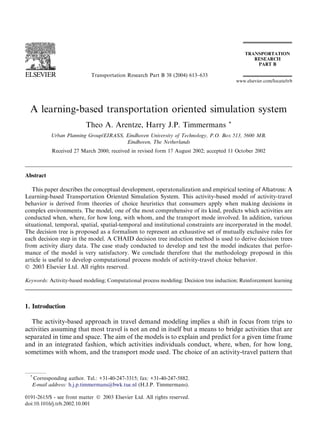
Fig. 1 schematically shows the process model. The model first decides on the transport mode
for the work activity. Mode choice for work is considered the highest-priority decision because
this choice determines which person can use the car for a substantial part of the day in cases where
there is only one car and more than one driving license available in the household.
Step 2 determines the activity composition of the schedule. For each flexible activity category, a
decision whether or not to add an episode of that activity to S is made. If an activity is added,
travel party and duration of the activity are determined before a next activity category is con-
sidered. This reflects the assumption that travel party and duration further define the nature of the
activity. For example, individuals may consider a leisure activity of long duration together with
others as qualitatively distinct from a leisure activity of short duration performed alone. Duration
is determined in a qualitative way as a choice between a long, average and short episode. Each

Schedule skeleton Skeleton+activities Schedule+Tours

Next activity Next activity Next tour

no
Select
Time of day Mode

yes
Travel party
Next activity Next activity

yes
Duration Location1
Trip link

no
Add to Program
Location2

Skeleton+activities Schedule+Tours

Schedule+Tours+Mode+Location

Fig. 1. The scheduling process model (Step 2–6).


duration class is defined by a time range depending on the activity category under concern.
Temporal constraints define the feasibility of both selection and duration decisions in this step.
Step 3 determines the time of day for each flexible activity in order of priority. This is modelled
as choosing a time period for the activity, based on a given subdvision of the day (e.g., early
morning, late morning, around noon, etc.). The time period constrains the start time of the ac-
tivity. Based on this the model determines a preliminary position in the schedule. In some cases,
the choice of time-of-day uniquely determines a position. In other cases, there remains a choice
between several feasible positions. In these cases, the model chooses the position with the shortest
time window, to maximize freedom of choice for next activities.
Step 4 determines trip links between activities by choosing for each activity in order of priority
whether it is conducted on a before stop (directly before another out-of-home activity in the
schedule), an after stop (directly after another out-of-home activity), an in-between stop or on a
single stop trip. The choices made in this stage have several implications for the schedule. First,
the activity is repositioned if needed to realize the chosen trip link. After this step, the position of
the activity is considered definite. Each activity with a definite schedule position can serve as a
basis for a trip link for activities considered next. Thus, trip links can be established between
flexible activities as well. Second, in-home activities are inserted where needed to make the
schedule consistent with chosen trip links.
In this stage, the tours included in the schedule are identifyable as sequences of one or more
out-of-home activities that start at home and end at home. Step 5 involves a choice of a transport
mode for each tour assuming that there are no mode changes between trips within tours. Tours
including a work activity take on the mode that was chosen for the work activity in the first step.
Finally, Step 6 determines the location of each flexible activity in order of priority. For each
location choice, the system defines a dynamic location choice-set, dependent on the time-window
for the activity, available facilities, opening times of facilities, travel times and minimum activity
duration. The decision is modeled as a choice among possible heuristics for selecting a location.
The heuristics define alternative ways of trading-off travel distance against attractiveness. Because
individuals may choose also inferior locations in terms of these characteristics (e.g., travel longer
for a less attractive location), the option ÔotherÕ is included. If ÔotherÕ is chosen, the model chooses
a travel-time band in which the destination location falls. If there is more than one location in the
choice set within the chosen band, the location is determined randomly.
The model constructs a schedule for each (adult) person in the household simultaneously by
alternating decisions between persons. For each person and each step, the model takes the
schedule of the partner as far as developed at the end of the previous step as input to take possible
interactions of scheduling choices between persons into account. Finally, we note that start time
and duration of flexible activities are not exactly determined by the model. With regard to start
time, the time-of-day and trip between activities are known. Hence, unless the activity is linked
with a fixed activity (with presumably known start and end time), there still remains a choice of
start time within some range. The same holds for duration.
In each step, dynamic constraints determine which choice alternatives are feasible given the
current state of the schedule. In many cases there will be a choice left and the decision tree linked
to that step is consulted to generate a choice. Socio-economic attributes of the person and
household are input to take possible interindividual differences in choice heuristics into account.
History dependence of decisions is taken into account by including outcomes of previous deci-


sions as input to each current decision. In this way, for example, the probability of adding
an activity will be strongly reduced when an activity of that category already has been added
in a previous step.

3.3. The inference system

This model component represents dynamic constraints of the types described in Section 2. For
each decision, the model evaluates dynamic constraints to determine the feasibility of choice al-
ternatives. The implementation of situational, household and temporal constraints is straight-
forward. This section focuses on space–time constraints and choice heuristics determining
location choices (Step 6).
A location l is considered feasible if the following two conditions are met:
9g 2 Gl ; g 2 GfaðsÞg ð1Þ
Tlfg max ðsÞ À Tlsgmin ðsÞ 6 vmin ðsÞ ð2Þ

where, s is an index of activities in a given schedule S, Gl is the set of known facility types at
location l, GfaðsÞg is the set of facilities compatible with activities of type aðsÞ, vmin ðsÞ is the
minimum duration and Tlsgmin and Tlfg max define the time window for the activity dependent on the
current schedule and opening hours of facilities. The latter terms are formally defined as

Tlfg max ðsÞ ¼ maxfd tlg ; T f min ðs À 1Þ þ tl ðsÞg
min t
ð3Þ
Tlsgmin ðsÞ ¼ minfd tlg ; T s max ðs þ 1Þ À tl ðs þ 1Þg
max t
ð4Þ
min max
where, d tlg and d tlg are the known opening and closing times of facilities of type g at location l
f min
on day d, T is the earliest end time and T s max the latest start time of the previous and next
t
activity respectively and tl is travel time to the activity location using the mode chosen in a
previous step. Earliest start times and latest end times of activities are calculated by shifting
previous activities as far as possible to the right on the time scale and next activities as far as
possible to the left within temporal constraints.
Having defined the location choice set, the proposed set of heuristics then define alternative
ways of trading-off required travel time against attractiveness of locations. Before formulating the
heuristics, two concepts must be clarified. First, the order of locations refers to an ordinal
judgement of the attractiveness of facilities at a location. The classification may relate to a hi-
erarchy of locations. For example, in the Dutch context, shopping centers can be classified into
three or four orders that range from neighborhood centers to city centers. The assumption here is
that individuals tend to evaluate alternative locations in such qualitative terms. Second, a location
is considered inferior if it is dominated by at least one alternative in terms of both travel time
(shorter) and order (higher). For example, l1 is dominated by l2 if l1 incurs more travel time and is
of lower or equal order compared to l2 Because different people may view order of places types
differently, the system uses a model that predict perceived order of place type as a function of
attributes of the location and person attributes for each activity category.
Let L be the choice set for the given activity defined by Eqs. (1)–(4), Lþ L be the subset of
t
non-inferior locations, tl be the travel time to location l, r1 r2 r3 Á Á Á rm be pre-defined


critical travel times of increasing lengths, Rr L be the subset of locations reachable within travel
time r. Then, the heuristics can be written as
h1 : choose location l if l 2 Lþ ^ tl ¼ minl0 2L ðtl0 Þ
t t
þ
h2 : choose location l if l 2 L ^ ol ¼ maxl0 2L ðol0 Þ
h3:1 : choose location l if l 2 Lþ ^ l 2 R1 ^ ol ¼ maxl0 2R1 ðol0 Þ
h3:2 : choose location l if l 2 Lþ ^ l 2 R2 ^ ol ¼ maxl0 2R2 ðol0 Þ
...
h3:m : choose location l if l 2 Lþ ^ l 2 Rm ^ ol ¼ maxl0 2Rm ðol0 Þ
h4 use some other heuristic
The first two heuristics represent extreme cases where individuals minimize travel time irre-
spective the order of locations (h1 ) or maximize order irrespective required travel time (h2 ). The
heuristics h3:1 –h3:m represent the choice for some optimum taking both travel time and order
into account. They define a maximum travel time and select the location that maximizes the
order within reach. As a set, the heuristics h3:1 –h3:m represent an increasing willingness to travel
further in order to reach locations of higher order. In all these heuristics non-inferiority is
included as a condition to make sure that a possible tie on one criterion (e.g., same travel time)
is resolved by a non-inferior choice on the other criterion (e.g., higher order). However, in-
dividuals do not necessarily select only non-inferior locations. The last heuristic covers the case
where individuals choose an inferior location possibly based on characteristics not represented
in the model.
It is easy to verify that heuristics h1 –h3:m may overlap in the sense that, dependent on choice-set
L, multiple heuristics may identify the same location. For example, the nearest location and the
highest order location may be the same location. To resolve such ambiguities, the proposed model
ranks heuristics based on a criterion of explanatory simplicity. The Ônearest locationÕ rule (h1 ) is
considered simpler than the maximum-travel-time rule, which in turn is considered simpler than
the Ôhighest-orderÕ rule (h2 ). If a conflict arises, the simplest heuristic is taken as the rule underlying
the observed choice.
Furthermore, it is easy to see that the set of heuristics is not exhaustive in the sense that it not
necessarily covers all locations in the choice-set. Let Lh represent the subset of locations that are
defined by at least one of the heuristics. Then, the complementary subset Lo consists of locations
that are inferior or lie beyond a maximum travel-time. Clearly, individuals may also select inferior
locations, for example, a location that performs highly on some other unknown attribute, or use
different travel time upper limits. To cover such cases, the proposed model considers a comple-
mentary set of heuristics that operates on Lo and considers travel time only. The ith heuristic
of this set considers the subset of locations of Lo that ly in the ith travel time band and selects
from this subset a random location.
Both sets of heuristics assume that individuals evaluate distances to locations in the context
of a tour that may consist of multiple activities. Alternatively, individuals may (conditionally)
use home-based travel time as a criterion for location selection even if the preceding location or
the next location differs from the home location. Therefore, the above set of heuristics (h1 –h4 )
can be complemented with an equivalent set based on home-based travel times. We assume that
home-based rules are simpler than the tour-based equivalents and, therefore, have higher pri-
ority.


4. Decision tree induction

The oval boxes in Fig. 1 indicate the places where a decision tree delivers input. This section
outlines an approach to derive the decision trees from data and develops a rule for deriving de-
cisions from induced trees. First, we discuss some relevant properties of this rule-based formalism.

4.1. The rule-based formalism

As we argued in Section 2, choice behavior that emerges from learning is driven by individual
dependent condition–action rules. In general format, a condition–action rule can be described as
if C1 2 CS1k ^ C2 2 CS2k ^ Á Á Á ^ Cm 2 CSmk then choose alternative Ak ð5Þ
where Ci represents condition variables, CSik the condition state of the ith variable in the kth rule
and Ak the choice generated by the kth rule. In this notation, a condition state is represented as a
subset of the domain of the condition variable. If the condition variable is of a nominal mea-
surement scale, then it may specify any subset of the domain. In the case of an ordinal or metric
variable, on the other hand, the condition state specifies a certain subrange of the variableÕs
domain.
To make sure that a rule set is able to respond to every situation, it must meet requirements of
completeness and consistency. A model is considered complete if at least one rule responds and
consistent if no more than one rule responds to every possible combination of values of condition
variables Ci . These properties are guaranteed by the way the learning mechanism operates in our
model. Consider an initial situation where the individual has no a-priori knowledge of the
domain. Decision-making would be purely random and handled by a single ÔruleÕ:
if C1 2 CD1 ^ C2 2 CD2 ^ Á Á Á ^ Cm 2 CDm then choose random ð6Þ
where CDi represents the domain of condition variable Ci . Since every Ôcondition stateÕ in this rule
equals the entire domain, each variable in effect is irrelevant. Therefore, every possible state in
terms of Ci will trigger the rule implying that the model meets the requirements of completeness
and consistency. Now assume that through interaction with the environment the individual has
learned to discriminate between states on some condition variable. This can be represented
by splitting the domain of that variable into two states so that the initial rule is replaced by two
new rules:
if C1 2 CD1 ^ C2 2 CD2 ^ Á Á Á Á Á Á ^ Cj 2 CSj1 ^ Á Á Á ^ Cm 2 CDm then choose A1 ð7Þ
if C1 2 CD1 ^ C2 2 CD2 ^ Á Á Á Á Á Á ^ Cj 2 CSj2 ^ Á Á Á ^ Cm 2 CDm then choose A2 ð8Þ
Because the new condition states were achieved by splitting a domain, CSj1 [ CSj2 ¼ CDj and
CSj1 CSj2 ¼ ; and, hence, the new model still meets properties of completeness and consis-
tency. 1 This process of splitting could be repeated endlessly resulting in increasingly complex
models while maintaining the required properties.

1
Our definitions of completeness and consistency do not have any implications for the action section. Although
it would not make sense in this example, the two rules could still specify the same action.


Besides properties of completeness and consistency, this simple case illustrates that the for-
malism is consistent with learning theory. Split operations that determine the selection of context
and choice attributes an individual evaluates for making a choice may differ from case to case. If
search behavior is extensive, condition states are split up to the extent required by the complexity
of condition-reward contingencies in the environment. On the other hand, tendencies of limited
exploration result in simpler rule sets.

4.2. Inducing decision trees from data

Any set of rules that can be obtained by recursively splitting condition states starting with an
initial rule of format (6) meets the formal definition of a decision tree as formulated by Sa-
favian and Landgrebe (1991) and vice versa. Methods based on principles of supervised
learning have been developed in statistics and artificial intelligence to empirically estimate
decision trees. Supervised learning is learning from examples with known outcomes (in this
case, observed behavior). Note that this class of learning is distinct from reinforcement and
social learning, where the right answers are unknown and only utilities are fed back to actions
of the individual. Hence, the supervised learning technique used here to derive decision trees
from data is not seen as a model of a learning process. Rather we use the technique to find the
tree that best describes observed choices. The outcome is considered a model of the current
state of knowledge of the individual or group of individuals from which observations were
taken. In case of a group of individuals, socioeconomic attributes are included as additional
condition variables available for splitting so that group heterogeneity in decision rules can be
represented in the model.
Examples from which a decision tree is induced describe observations on one or more condition
variables (our terminology) and a single response variable. The (minimal) tree that partitions the
sample into groups that are maximally homogeneous in terms of the response variable is con-
sidered the best hypothesis for the data. Because the number of possible trees increases expo-
nentially with the number of condition variables, work in this area has focused on heuristics to
search for the best tree. C4.5 (Quinlan, 1993), CART (Breiman et al., 1984) and CHAID (Kass,
1980) are the most widely used heuristics. 2 All three programs grow a tree from the root by
recursively splitting the sample on one condition variable at a time. They differ with respect to the
criterion that is used for evaluating possible splits. C4.5 uses an entropy measure and CART the
Gini-index to measure purity of a response distribution, whereas CHAID evaluates splits based
on a Chi-square measure of significance of differences in response distributions between groups.
CHAID further differs in that it uses a stop rule, whereas the other programs first grow a full tree
and next prune the tree by removing insignificant branches.
The choice of an induction method for developing Albatross is based on a trade-off between
specific strengths of the competing methods. A two-staged process, as employed by C4.5 and
CART, is potentially more powerful, because it circumvents to some extent the inherent weakness

2
CHAID is usually not considered as a decision tree induction method as it was introduced in statistics as a data
segmentation technique. However, because the form of input and output is the same, we consider CHAID to belong to
this class of methods (Arentze et al., 2000).


of looking only one step ahead in selecting splits. By lowering the threshold for splitting in the
tree-growing stage splits that pay-off only in combination with other splits are more likely to be
identified. On the other hand, CHAID is more sensitive for differences in complete response
distributions compared to C4.5 and CART. The entropy measure and Gini-index do take entire
response distribution into account in the growing stage. However, the effects are counterbalanced
in the pruning stage, where both methods base pruning decisions primarily on (absence of) dif-
ferences in modal responses alone.
Arguably, the latter disadvantage of C4.5 and CART outweighs the advantage of a two-staged
approach. A model of modal responses ignores residual variance in responses within the partitions
created. As will be explained in the next section, Albatross uses a probabilistic rule for assigning
responses to cases classified by a tree with the aim to reproduce non-systematic variance in model
predictions. In the context of a probabilistic rule the distribution of responses is as important as
the modal response. Moreover, in previous comparative studies (Arentze et al., 2000 and Wets
et al., 2000) we found no significant differences in performance between the methods on an
activity-data set. It is for that reason that we propose CHAID for developing decision-tree based
models such as Albatross.

4.3. Deriving decisions from decision trees

Having derived a decision tree for each choice facet, the next question becomes how to derive
decisions from trees for prediction. Consider a response variable that has Q levels and for which
CHAID produced a tree with K leaf nodes. In the prediction stage, the tree is used to classify new
cases to one of the K leaf nodes based on attributes of the case. A response-assignment rule needs
to be specified that defines a response (decision) for each classified case. In many applications, a
plurality rule is used. This rule assigns the modal response among training cases (i.e., the sample
used for developing the tree) at a leaf node. A deterministic rule like this may yield the best
predictions at an individual level, but fails to reproduce residual variance (if any) at leaf nodes
in predictions. Given our modeling purpose, we, therefore, use a probabilistic assignment rule
instead. According to this rule, the probability of selecting the qth response for each new case
assigned to the kth node is simply given by

fkq
pkq ¼ ð9Þ
Nk

where fkq is the number of training cases of category q at leaf node k and Nk the total number
of training cases at that node.
This rule is sensitive to residual variance, but fails to take scheduling constraints into account.
Scheduling constraints entail that dependent on individual attributes and the state of the current
schedule some choice alternatives for the decision at hand may be infeasible. If such constraints
are represented in the decision tree, the probabilistic rule would assign zero probability to in-
feasible categories and the response distribution should not be biased. However, even though it is
likely, it is not guaranteed that the induction method discovers constraint rules in data. Therefore,
to cover the general case we need to refine rule (9) as

(
0 if q is infeasible
pkq ¼ Pfkq otherwise ð10Þ
f 0
q0 kq

where q0 is an index of feasible alternatives for the decision at hand. Even though this rule may
work well in practice, it may produce slightly biased patterns at an aggregate level that should be
noted. That is to say, the rule tends to overpredict responses that are feasible in the majority of
cases (at that leaf node), because the probability of these responses is increased by rule (10) in
constrained cases and stays the same as (9) in unconstrained cases. Nevertheless, we use rule (10)
keeping in mind that improvements are possible.

5. Application

To develop and test the Albatross model, an activity diary survey was conducted in two mu-
nicipalities in the Rotterdam region in the Netherlands in 1997. This section discusses the format
of the diary data and results of decision tree induction.

5.1. Data

The survey invited households to fill out an activity diary for two consecutive days. Days were
designated to households such that the sample was balanced across the days of the week. The
activity diary asked respondents, for each successive activity, to provide information about the
nature of the activity, start and end time, the location where the activity took place, the transport
mode (chain) and the travel time per mode, if relevant, accompanying individuals (alone, other
member of household, other), and whether the activity was planned. Open time intervals were
used to report the start and end times of activities. A pre-coded scheme including 48 categories
was used for activity reporting. Response rates among households that had indicated to be willing
to participate ranged between 64% and 82% dependent on mode of administration. This resulted
in a total of 2198 household-days that were used for the analysis. The diaries were cleaned using
the special-purpose program Sylvia (Arentze et al., 1999).
Data of the physical environment were obtained through national databases and fieldwork. The
data were aggregated to zip-code zones and included mode-specific shortest-route travel times and
distances between zones, size of facilities by sector and opening hours of facilities by sector and
day of the week. The size of facilities was measured as total amount of floor space and number of
employees per sector. Opening hours data were collected through local inspection of centers and a
telephonic survey among outlets, chains and organizations. They were aggregated per zone by
calculating the earliest possible opening time and latest possible closing time across outlets. The
types of facilities considered included daily shopping, non-daily shopping, service (bank, post
office, travel agency, etc.) and leisure facilities (cafe, restaurants, theatre, etc.).
The 48 activity categories used in the diary were classified into 11 broader categories. Table 1
shows the classification used and subdivision into fixed and flexible activities. All flexible out-of-
home activities could be related to facilities in the physical data set, except social activities. With
respect to social activities, the model assumed that all zones and times are feasible and equally
attractive for conducting the activity.


Table 1
Classification of activities used in the Albatross model
Fixed activities Flexible activities
Work/school Daily shopping
Bring or get persons or goods Service related activities (post office, bank etc.)
Medical visits Non-daily shopping
Personal business (a rest category) Social activities (visiting friends, relatives etc.)
Sleep and eat Leisure activities (sports, concert, library, restaurant etc.)
Home-based activities (other than sleep and eat)

5.2. Results of decision tree induction

The activity diary data was used to derive a decision tree for each decision step in the process
model (see Section 3) conveniently assuming that reported activities reflected the activity sched-
ules of individuals. 3 75% of the cases was used for training (developing the decision trees) and the
remaining cases were used for validation testing. For each choice facet, the observed choice and
attributes of the schedule as far as known in that stage of the assumed decision process were
extracted from the diary data.
In general, the attributes considered as potentially relevant condition variables relate to:

1. Person, household and space–time setting;
2. Activity program/sequence at schedule level (including partner, if any);
3. Activity program/sequence at tour level;
4. Activity profile and space–time setting at activity level;
5. Feasibility of choice alternatives at choice-facet level.

Socio-economic and space–time setting attributes at person and household level allow CHAID
to identify groups of individuals with similar choice behavior. Thus, deriving decision rules and
segmenting the population in homogeneous groups in terms of these decision rules is accom-
plished simultaneously. Available information at schedule, tour, and activity level is initially
limited to the schedule skeleton and increases as scheduling proceeds. Because outcomes of
previous decisions are included as conditional variables for each next decision step, interactions
between choices can be represented explicitly in decision trees. Finally, the last category––feasi-
bility of choice alternatives––is important, because it allows the system to differentiate between
choice behavior under constrained and unconstrained conditions.
CHAID allows users to define the threshold for splitting in terms of a significance level for the
v2 measure and a minimum number of cases at leaf nodes. Alpha was set to 5% and the minimum
number of cases to 20. Because CHAID can handle categorical condition variables only, con-
tinuous attributes such as travel times, durations and start times, were discretisized using an

3
In reality, not necessarily all activities that people conduct are planned. Furthermore, during execution the schedule
can be adjusted in response to unforeseen events.


Table 2
Results of inducing decision trees from diary data by choice facet
Decision tree N alts N cases N Attr N leafs hit r(0) hit r(t) hit r(v)
1. Mode for work 4 858 32 23 0.525 0.648 0.667
2. Activity selection 2 14,190 40 116 0.669 0.724 0.716
3. Activity, with-whom 3 2970 39 57 0.335 0.509 0.484
4. Activity, duration 3 2970 41 61 0.334 0.413 0.388
5. Activity, time-of-day 6 2970 62 86 0.172 0.398 0.354
6. Trip link 4 2651 52 30 0.533 0.833 0.809
7. Mode for other 4 2602 35 65 0.388 0.528 0.495
8. Activity, location 1 7 2112 28 62 0.375 0.575 0.589
9. Activity, location 2 6 1027 28 34 0.326 0.354 0.326
N alts: number of choice alternatives; hit r (0): expected ratio of correctly predicted cases (null model); N cases: number
of training cases; hit rðtÞ: expected ratio of correctly predicted cases (training set); N attr: number of attributes; hit rðvÞ:
expected ratio of correctly predicted cases (test set); N leafs: number of leaf nodes.

equal-frequency method. This method divides a scale into n parts in such a way that each part
represents approximately the same number of cases.
Table 2 shows input and output characteristics of CHAID per decision tree. The number of leaf
nodes gives an indication of the complexity of the resulting tree and the last three columns shows
hit ratios as a measure of predictive accuracy. The hit ratio represents the expected number of
correctly predicted cases when a probabilistic response-assignment rule of type (9) is used. It is
P ðfkq Þ2
calculated as kq Nq where fkq is the frequency of the qth response at the kth leaf node and Nk is
the frequency of the qth response in the entire sample.
As it turns out, performance varies considerably across choice facets. Duration, with-whom,
location (2) and time-of-day choices are relatively difficult to predict. Partly, this reflects differ-
ences in number of choice alternatives. The base probability of correctly predicting choices in-
creases with decreasing number of alternatives. Comparison with expected hit ratios of a null
model gives an indication of relative performance. The null model uses the probability distribu-
tion at the aggregate level to predict a choice in each case and, hence, simulates a tree with a single
leaf node. Relative performance is relatively poor for activity-selection and duration facets and
relatively good for location and time-of-day choices. Finally, comparing expected hit ratios be-
tween training and test set gives an indication of generalizability of the model to unseen cases.
Since decline in performance is generally small, we conclude that overfitting is not a problem here.
Each decision tree provides valuable information for interpreting choice behavior. To illustrate
the use of trees for interpretation, Table 3 shows a branch of the time-of-day tree as an example.
The first split in this tree concerns activity type and the branch depicted relates to non-daily
shopping activities. The (sub)tree is represented in table format. The upper section of the table
shows condition variables and condition states and the bottom section displays the levels of the
response variable and response probability distributions of training cases. Note that each column
corresponds with a leaf node. The last row shows number of training cases per leaf node.
As can be concluded from the table, time-of-day choices for non-daily shopping are condi-
tioned almost exclusively by patterns of available time in the current schedule. Tmax variables
represent for each of four episodes of the day whether and to what extent there is time to conduct


Table 3
Example of a decision tree: time-of-day of non-daily shopping activities
yDshop – – – – – 0 1 – – 0 0 1
yLeis – – – – – – – – – 0 1 –
Tmax1 0 0 0 0 0 0 0 1 2–3 2–3 2–3 2–3
Tmax2 0 0 0 0 1–2 3 3 – – – – –
Tmax3 0 0 1–2 3 – – – – 0 1–3 1–3 1–3
Tmax4 0 1–3 – – – – – – – – – –
10 am 0.00 0.00 0.00 0.00 0.00 0.00 0.00 0.32 0.25 0.16 0.08 0.05
10–12 am 0.00 0.00 0.00 0.00 0.41 0.47 0.23 0.37 0.29 0.15 0.42 0.13
12–2 pm 0.00 0.00 0.90 0.40 0.35 0.13 0.23 0.21 0.00 0.34 0.14 0.42
2–4 pm 0.00 0.81 0.11 0.48 0.24 0.22 0.50 0.05 0.21 0.27 0.33 0.30
4–6 pm 0.50 0.12 0.00 0.04 0.00 0.18 0.05 0.05 0.14 0.08 0.03 0.05
6 pm 0.50 0.08 0.00 0.08 0.00 0.00 0.00 0.00 0.11 0.00 0.00 0.06
N 30 26 19 25 37 60 22 19 28 74 36 64
yDshop: there is a daily shopping activity in the schedule (0 ¼ no, 1 ¼ yes); yLeis: there is a out-of-home leisure activity
in the schedule (0 ¼ no, 1 ¼ yes); Tmax1–4: available time in the widest open time slot within episode 1–4 of the day
(0 ¼ insufficient, 1 ¼ sufficient and 2 ¼ more than sufficient).

the shopping activity (with duration given by a previous decision). As an overall rule, the model
tends to select the earliest feasible episode of the day. However, in cases where this episode starts
before 12 pm, time-of-day choices become more dispersed. Under less constrained choice situa-
tions the preferred time of day stretches from 10 am to 4 pm. The presence of an out-of-home
daily shopping activity tends to delay non-daily shopping, whereas the presence of an out-of-
home leisure activity tends to lead to earlier start times. In sum, the patterns suggest specific
preferences for time-of-day and sequencing of activities and point at a strong influence of tem-
poral constraints. Socio-demographic and space–time setting attributes do not provide additional
explanation of choice behavior in this case.

6. Performance of the Albatross model

The hit ratios shown in Table 2 give an indication of prediction accuracy of each decision tree
whereby earlier decisions are given as observed. Choices between choice facets are, however,
interrelated in the sense that earlier decisions affect conditions for later decisions. Moreover,
decisions derived from trees are part of a scheduling process model that translates decisions to
appropriate operations on the schedule. The eventual goodness-of-fit of the model can be as-
sessed only by a comparison at the level of complete activity patterns. Being a travel demand
model, the eventual output of Albatross consists of trip matrices. This section evaluates good-
ness-of-fit at this level. Before discussing the results, we consider some descriptive statistics of the
data.
Table 4 shows the means and standard deviations of number of activities of predicted and
observed patterns. Because Albatross does not differentiate between in-home activities, consec-
utive in-home activities in observed patterns were merged to make the sets comparable. After this


Table 4
Mean number of elements in patterns (standard deviation between brackets)
Training data Test data
Observed Predicted Observed Predicted
N activities (total) 5.328 (2.653) 5.357 (2.817) 5.230 (2.540) 5.441 (2.762)
N activities (flexible) 1.343 (1.213) 1.293 (1.247) 1.287 (1.174) 1.352 (1.269)

pre-processing, the mean length of patterns varies between 5.2 and 5.4 activities dependent on the
data set. Recall that Albatross considers fixed activities as given. The mean number of flexible out-
of-home activities varies between 1.3 and 1.4. The means as well as standard deviations are fairly
accurately predicted, be it that the number of activities is slightly overpredicted in the test set.
The study area counts 19 zones. The outside area is considered an additional single zone in the
trip matrix. Different matrices were generated varying a third dimension on which interactions
were broken down. The third dimensions considered include:

1. No third dimension;
2. Transport mode (slow mode, car driver, car passenger and public transport);
3. Day of the week (weekday, Saturday, Sunday);
4. Time of day (before 10 am, 10–12 am, 12–2 pm, 2–4 pm, 4–6 pm, after 6 pm);
5. Activity (nine categories);
6. Activity (only flexible activities: five categories).

Note that the number of cells and, hence, the degree of disaggregation differs between the
matrices. For example, the trip matrix by mode has 4 · 20 · 20 ¼ 1600 cells and the trip matrix by
activity has 9 · 20 · 20 ¼ 3600 cells. The fifth and last matrix is based on trips with a flexible
activity at the destination location only. This matrix is particularly relevant for assessing the
performance of the model, because it leaves out trips with locations and activities given by
the skeleton.
The correlation coefficient was used as a measure of degree of correspondence between trip
matrices. As Table 5 shows, correlations for the test set vary between 0.706 and 0.954 dependent
on the third dimension. The variation across matrices can be largely explained by the variation in
number of cells. As could be expected, goodness-of-fit decreases with increasing number of cells
(i.e., the level of disaggregation of interactions). Furthermore, as expected the matrix related to

Table 5
Contingency and correlation measures between predicted and observed OD matrices
Training data Test data
None 0.966 0.954
Mode 0.933 0.887
Day 0.969 0.962
Time of day 0.970 0.953
Activity 0.896 0.845
Activity (flex) 0.832 0.706


flexible activities shows an extra decline in fit. Overall, however, the results indicate that per-
formance is very satisfactory keeping in mind that patterns are only partly predicted by the model.
The difference in performance between training and test set can be expressed as a ratio between
test-set and training-set scores. The ratios range between 85% and 99%. We conclude, therefore,
that the extent to which overfitting has occurred is acceptable.

7. Conclusions and discussion

This paper described the conceptual development, operationalisation and validation testing of
Albatross. The system simulates individualÕs decisions related to every facet of activity schedules
generally considered relevant for activity-travel analysis. The facets include activity type, dura-
tion, travel party, start time, trip type, location and transport mode. The system is designed as
a rule-based model in which situational, household, institutional and space–time constraints as
well as choice heuristics of individuals are explicitly represented in the system.
Central to the proposed approach is the use of the decision tree for representing choice heu-
ristics of individuals and deriving these heuristics from activity travel data. As it appeared, the
decision tree achieved a considerable, but varying improvement of predictive accuracy compared
to a null model and the results could be replicated on a validation set. Correlations between
observed and predicted trip matrices indicated that the model is able to explain a large proportion
of observed variance across intensities of trip flows disaggregated on various dimensions relevant
for travel analysis.
We conclude therefore that the approach is useful for developing computational process models
for forecasting travel demands. We motivated the choice for a rule-based approach based on a
theory of how people learn in complex environments. Potentially, decision trees are better able to
represent the heuristic and context dependent nature of choice behavior compared to current
utility-maximizing models. Although decision tree induction requires relatively large data sets,
this research shows that a sample size of the order of magnitude of 2000 household-days suffices
to develop a stable model and test the validity of the model. Nevertheless several issues remain
for future research.
First, the generalizability of the present model was tested on a holdout sample. Because the
holdout sample originated from the same study area and the same survey instrument, this is more
a test of internal validity than external validity. The question remains how well the model would
perform when applied in another study area. Transferability of a model to another context than in
which it was developed has received some attention in the area of discrete choice modeling
(Koppelman and Wilmot, 1982). Such transferability studies need to be replicated in this new area
of rule-based models. The ability to predict reactions of individuals to transportation or spatial
policy scenarios is a specific form of transferability that is of particular interest. On all of these
criteria of internal and external validity it is worth while to compare the rule-based approach with
equivalent utility-based models. Such comparative studies would provide an indirect test of
validity of the specific assumptions underlying the rule-based model.
Besides testing the current model, several extensions of the model are worth considering. First,
decision tree induction techniques use principles of supervised learning and, therefore, are not
suitable for modeling individuals time paths of learning and adaptation. To model time paths as


well, models of reinforcement and social learning need to be developed and incorporated in the
system. Potentially, the resulting dynamic model would be able to predict and analyze long-term
impacts of policy measures or trends in society.
Second, we mention possible extensions at the level of the process model. Although the current
process model is already quite comprehensive compared to existing activity-based models, several
extensions could increase sensitiveness of the model for relevant travel demand measures. These
cover areas of (1) joint decision making and interactions between persons within households, (2)
long-term decision making related to choice facets of the schedule skeleton, (3) re-scheduling
behavior during schedule execution, (4) individual and context varying styles of scheduling and (5)
in-home versus out-of-home activity substitution choice behavior.

References

Anderson, J.R., 1983. The Architecture of Cognition. Harvard University Press, London.
Arentze, T., Hofman, F., van Mourik, H., Timmermans, H., Wets, G., 2000. Using decision tree induction systems
for modeling space–time behavior. Geographical Analysis 32, 330–350.
Arentze, T.A., Hofman, F., Timmermans, H.J.P., 1999. System for the logical verification and inference of activity
(SYLVIA) diaries. Transportation Research Record 1660, 156–163.
Bhat, C.R., 1999. A comprehensive and operational analysis framework for generating the daily activity travel profiles
of workers. Paper presented at the 78th Annual Meeting of the Transportation Research Board, Washington, DC,
January 10–14.
Bhat, C.R., Koppelman, F.S., 2000. Activity based travel demand analysis: History, results and future directions. Paper
presented at the 79th Annual TRB Meeting, January 2000, Washington DC, US.
Breiman, L., Friedman, J.H., Olshen, R.A., Stone, C.J., 1984. Classification and Regression Trees. Wadsworth,
Belmont (CA).
Doherty, S.T., 2000. An activity scheduling process approach to understanding travel behavior. Paper presented at the
79th Annual TRB Meeting, January 2000, Washington DC, US.
Doherty, S.T., 2001. Classifying activities by scheduling time horizon using machine learning algorithms. Paper
presented at the 80th Annual Meeting of the Transportation Research Board, January 2001, Washington DC, US.
Ettema, D.F., Borgers, A.W.J., Timmermans, H.J.P., 1993. A simulation model of activity scheduling behavior.
Transportation Research Record 1413, 1–11.
G€rling, T., 1992a. Determinants of everyday time allocation. Scandinavian Journal of Psychology 33, 160–169.
a
G€rling, T., 1992b. The importance of routines for the performance of everyday activities. Scandinavian Journal of
a
Psychology 33, 160–169.
G€rling, T., 1998. Behavioural assumptions overlooked in travel-choice modelling. In: Ortuzar, J., Jara-Diaz, S.,
a
Hensher, D. (Eds.), Transport Modeling. Pergamon, Oxford, pp. 1–18.
G€rling, T., Br€nn€s, K., Garvill, J., Golledge, R., Gopal, S., Holm, E., Lindberg, E., 1989. Household activity
a a a
scheduling, In: Transport Policy, Management and Technology Towards 2001, Vol. IX, Contemporary
Developments in Transport Modeling, WCTR, Yokohama, pp. 235–248.
G€rling, T., Gillholm, R., Montgomery, W., 1999. The role of anticipated time pressure in activity scheduling.
a
Transportation 26, 173–192.
G€rling, T., Gillholm, R., Romanus, J., Selart, M., 1997. Interdependent activity and travel choices: behavioural
a
principles of integration of choice outcomes. In: Ettema, D.F., Timmermans, H.J.P. (Eds.), Activity-based
Approaches to Activity Analysis. Pergamon Press, Oxford, pp. 135–150.
G€rling, T., Kaln, T., Romanus, J., Selart, M., 1998. Computer simulation of household activity scheduling.
a e
Environment and Planning A 30, 665–679.
G€rling, T., Kwan, M.-P., Golledge, R.G., 1994. Computational-process modeling of household travel activity
a
scheduling. Transportation Research B 25, 355–364.


Golledge, R.G., Kwan, M.-P., G€rling, T., 1994. Computational process model of household travel decisions using a
a
geographic information system. Papers in Regional Science 73, 99–118.
Kass, G.V., 1980. An exploratory technique for investigating large quantities of categorical data. Applied Statistics 29,
119–127.
Kitamura, R., Fujii, S., 1998. Two computational process models of activity-travel behavior. In: G€rling, T., Laitila, T.,
a
Westin, K. (Eds.), Theoretical Foundations of Travel Choice Modeling. Elsevier, Amsterdam, The Netherlands,
pp. 251–280.
Koppelman, S., Wilmot, C.G., 1982. Transferrability analysis of disaggregate choice models. Transportation Research
Record 895, 18–24.
Kwan, M.-P., 1997. GISICAS: an activity-based travel decision support system using a GIS-interfaced computational
process model. In: Ettema, D.F., Timmermans, H.J.P. (Eds.), Activity-based Approaches to Activity Analysis.
Pergamon Press, Oxford, pp. 263–282.
Quinlan, J.R., 1993. C4.5 Programs for Machine Learning. Morgan Kaufmann Publishers, San Mateo (CA).
Recker, W.W., McNally, M.G., Root, G.S., 1986a. A model of complex travel behavior: Part 1: Theoretical
development. Transportation Research A 20, 307–318.
Recker, W.W., McNally, M.G., Root, G.S., 1986b. A model of complex travel behavior: Part 2: An operational model.
Transportation Research A 20, 319–330.
Safavian, S.R., Landgrebe, D., 1991. A survey of decision tree classiﬁer methodology. IEEE Transactions on Systems
Man and Cybernetics 21, 660–674.
Sutton, R.S., Barton, A.G., 1998. Reinforcement Learning: An Introduction. MIT Press, London.
Vause, M., 1997. A rule-based model of activity scheduling behavior. In: Ettema, D.F., Timmermans, H.J.P. (Eds.),
Activity-based Approaches to Activity Analysis. Pergamon Press, Oxford, pp. 73–88.
Wets, G., Vanhoof, K., Arentze, T., Timmermans, H., 2000. Identifying decision structures underlying activity patterns:
an exploration of data mining algorithms. Transportation Research Record 1718, 1–9.

A learning based transportation oriented simulation system

Recomendados

Recomendados

Mais conteúdo relacionado

Mais procurados

Mais procurados (15)

Destaque

Destaque (9)

Semelhante a A learning based transportation oriented simulation system

Semelhante a A learning based transportation oriented simulation system (20)

Último

Último (20)

A learning based transportation oriented simulation system