Javier Garcia - Verdugo Sanchez - Six Sigma Training - W4 The Binary Logistic Regression

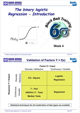
/4304 BB W4 Logistic Regression 07, D. Szemkus/H. Winkler
The binary logistic
Regression - Introduction
0
1
)(aP
a
Week 4
Page 2/4304 BB W4 Logistic Regression 07, D. Szemkus/H. Winkler
Factor X = Input
Discrete / Attributive Continuous / Variable
ResponseY=Output
Discrete
Attributive
Continuous
Variable
Chi - Square
Logistic
Regression
T - Test
ANOVA ( F - Test)
Median Tests
Regression
Statistical techniques for all combination of data types are available
Validation of Factors Y = f(x)

Lets assume we investigate parts from three different
suppliers.
What is the relation or odds of “bad” parts to “good”
parts for each supplier
An Example
Supplier x y z
Bad parts 41 48 40
Good Parts 29 32 10
Odds (Supplier X) = 41/29
29 parts good
41 parts bad
Relationship between ProbabilitiesProbabilities and OddsOdds:
P(Y=i) O(Y=i)
0,00% 0,00
5,00% 0,05
10,00% 0,11
15,00% 0,18
20,00% 0,25
25,00% 0,33
30,00% 0,43
35,00% 0,54
40,00% 0,67
45,00% 0,82
50,00% 1,00
55,00% 1,22
60,00% 1,50
65,00% 1,86
70,00% 2,33
75,00% 3,00
80,00% 4,00
85,00% 5,67
90,00% 9,00
95,00% 19,00
100,00% 999999,00
Thinking in Odds is different
and needs some time getting
used to it.
Probability to pick a bad Part
of e.g. 60% means,
the odds to pick a bad Part is
1,5 higher that to pick a good one.
00
+∞+∞
00
11
Motivation for using Odds
P(Y=i)
1 - P(Y=i)Odds(Yi) :=

Supplier Odds
X 41/29 = 1,41
Y 48/32 = 1,50
Z 40/10 = 4,00
We can calculate the odds
for all three suppliers
An Example, the Odds
Supplier x y z
Bad parts 41 48 40
Good Parts 29 32 10
Odds for a bad part of Y = 48/32 = 1,50
Odds for a bad part of X = 41/29 = 1,41
Odds ratio (Y vs. X) = 1,50/1,41 = 1,06
The odds ratio is the
ratio of the odds itself
Definition: Odds Ratio
Supplier x y z
Bad parts 41 48 40
Good Parts 29 32 10

Odds Ratio (Y relative to X) = 1.06
Odds Ratio (Z relative to X) = 2.83
Odds Ratio (Z relative to Y) = 2.67
Are the three suppliers different?
Therefore we have to calculate the confidence
intervals for the odds ratios!
We can calculate the following odds ratios:
Odds Ratio
95% confidence intervals of the Odds Ratio for Y relative to X
)03,255,0(
32
1
48
1
29
1
41
1
96.1
29/41
32/48
lnexp
32
1
48
1
29
1
41
1
29/41
32/48
lnexp
2/1
2/1
/21
−=
⎥
⎥
⎦
⎤
⎢
⎢
⎣
⎡
⎟
⎠
⎞
⎜
⎝
⎛
+++±⎟
⎠
⎞
⎜
⎝
⎛
=
⎥
⎥
⎦
⎤
⎢
⎢
⎣
⎡
⎟
⎠
⎞
⎜
⎝
⎛
+++±⎟
⎠
⎞
⎜
⎝
⎛
−αZ
Odds Ratio Confidence Intervals
Supplier x y z
Bad parts 41 48 40
Good Parts 29 32 10
Background: 95% CI for lognat(OR) = ± 1,96 * SEln(OR)
where SEln(OR) = 1010
1111
BBAA
+++

95%
confidence
interval
Odds Ratio lower upper
Y to X 0,55 2,03
Z to X 1,22 6,56
Z to Y 1,17 6,09
What is your conclusion for this example?
Rule: If the “1” is within the 95% confidence interval we can not say
that the suppliers are different in their capability.
Analog we can calculate confidence intervals for
Y relative to X and Z relative to Y
Odds Ratio Confidence Intervals
The “Log Odds Ratio” is the natural logarithm of the
Odds Ratio.
The “Log Odds Ratio” is a important metrics of the
logistic regression
Odds Ratio Log Odds Ratio
Y zu X 1,06 0,058
Z zu X 2,83 1,040
Z zu Y 2,67 0,982
Definition: Log Odds Ratio

Example in Minitab
Which factors
should be
considered in
the model?
Which of the
factors are
attributive?
Work sheet
“supplier.mtw”
Stat
>Regression
>Binary Logistic Regression…
Stat
>Regression
Logistic Regression Table
Odds 95% CI
Predictor Coef StDev Z P Ratio Lower Upper
Constant 0.3463 0.2426 1.43 0.154
Factor
Y 0.0592 0.3331 0.18 0.859 1.06 0.55 2.04
Z 1.0400 0.4288 2.43 0.015 2.83 1.22 6.56
Log-Likelihood = -126.348
Test that all slopes are zero: G = 7.499, DF = 2, P-Value = 0.024
P-values Odds
Ratios
Confidence
interval
Log Odds Ratios
Results in the Session Window
What is your conclusion for this example?

Example:
In an experiment 100 men were investigated if the suffer
from coronary heart disease (CHD).
⎩
⎨
⎧
⇒
⇒
=
diseased1
diseasednot0
responsetheisCHD
The development of a coronary heart disease depends
from many factors. One possible factor is the age.
The file CHD.mtw consists data of study in UK. 100 men has
been investigated. One possible input variable is the age and
the second one is the occurrence of the disease (1)
Binary Logistic Regression
The data of the
investigations are
stored in the Minitab
Worksheet
CHD.MTW.
ID Age CHD ID Age CHD ID Age CHD
21 20 0 22 37 1 36 52 0
76 20 0 27 37 0 2 53 1
4 25 0 42 37 1 63 53 0
14 25 0 60 37 0 95 53 1
26 25 0 64 37 0 99 53 1
66 25 0 84 37 0 40 54 1
69 25 0 52 38 0 24 55 0
19 26 0 33 39 0 85 55 1
78 26 0 47 39 1 94 55 1
5 28 0 53 39 0 12 56 1
51 28 0 97 39 0 6 57 1
55 28 0 54 40 0 45 57 1
44 29 0 86 40 1 59 57 1
80 29 1 79 41 1 72 57 1
7 30 0 83 41 0 75 57 0
8 30 0 16 42 0 87 57 0
17 30 0 74 42 0 98 57 1
23 30 0 82 42 0 31 58 1
30 30 0 92 42 1 68 58 1
35 30 0 96 42 0 77 58 1
37 30 0 13 45 0 88 58 1
65 30 1 20 45 0 91 58 0
67 30 0 93 45 1 39 59 1
90 30 0 61 46 0 49 60 1
29 32 0 3 47 0 10 62 0
1 33 0 43 47 1 25 62 1
18 33 0 46 47 0 57 62 1
56 33 0 81 47 1 62 63 1
34 35 0 28 48 1 73 63 1
70 35 0 41 48 0 38 64 0
71 35 0 50 48 0 89 64 1
100 35 0 15 49 0 48 65 1
9 37 0 32 49 1 58 65 1
11 37 0
Can we estimate
because of the
age the risk for a
heart disease?
The Investigation Data

How would you analyze the data?
Plot of the Investigation Data
706050403020
1,0
0,8
0,6
0,4
0,2
0,0
Age
CHD
Scatterplot of CHD vs Age
Probability for CHD for Each Group of Age
We get a curve with a S-shape
The data are combined in 8
groups and for each group a
group of age the risk can be
calculated
Group Mean CHD Mean Age
20-29 0.071 26
30-34 0.071 31
35-39 0.176 37
40-44 0.333 41
45-49 0.385 47
50-54 0.667 53
55-59 0.765 57
60-69 0.800 63
y
656055504540353025
0,8
0,7
0,6
0,5
0,4
0,3
0,2
0,1
0,0

0
1
The Logistic Response Function
The S-shaped curve
can be good
described with the
function (model)
a
a
e
e
aP 1
1
bb
bb
+
+
+
= 0
0
1
)(
P(a) = probability for coronary heart disease in the age a
)(aP
a
Logit - function
Logit Function
The coefficient of the logistic response function is called
“Logit Function”
( )[ ] [ ]abbabbagag 1010 1)()1( +−++=−+
abbag 10)( +=
If the age (a) changes by 1, g(a) changes by b1
abbbabb 10110 −−++=
1b=
Coefficient out of the regression equation
Variable, here the age

At the linear regression, is y(x+1) - y(x) = b1
the difference if x is increased by 1
At the logistic regression is g(x+1) - g(x) = b1
the difference if x is increased by 1
The model for the linear regression:
xbbxy 10)( +=
xbbxg 10)( +=
with y(x) = response function
with g(x) = logit function
The model for the logistic regression:
Linear Regression vs. Binary Logistic Regression
Link Function: Logit
Response Information
Variable Value Count
CHD 1 38
0 62
Total 100
Odds 95% CI
Predictor Coef StDev Z P Ratio Lower Upper
Constant -6.153 1.186 -5.19 0.000
AGE 0.12553 0.02487 5.05 0.000 1.13 1.08 1.19
Log-Likelihood = -47.437
Test that all slopes are zero: G = 37.939, DF = 1, P-Value = 0.000
Information in the session window
a
b
c
d
fe
The CHD Example
Stat
>Regression
Stat
>Regression
File: CHD.MTW

Information from the Session Window
a. Die response variable has only 2 values, 0 und 1
b. The coefficients of the model and standard deviation
The coefficients are:
c. Z – value of the normal distribution, the calculated p-value of the
coefficients (Z= Coef / StDev)
The Null hypothesis (H0): Coefficient = 0
Because of the p-value: reject H0 (at α = 0,05)
d. The confidence interval for the odds ratio is 1,08 and 1,19. The
best estimate for the odds ratio is 1,13
e. Minitab calculated the model coefficients due maximizing of the
log-likelihood function
f. The null hypothesis (H0): b0 = 0. If the null hypothesis is true, the
G-statistic uses a χ² distribution with 1 df. The H0 with a selected α
= 0.05 will be rejected
12553.0b153.6b 10 =−=
Plot of the Logistic Response Function
a
a
e
e
aP 12553.153.6
12553.153.6
1
)( 0
0
+−
+−
+
=
706050403020
0,9
0,8
0,7
0,6
0,5
0,4
0,3
0,2
0,1
0,0
Age
P(a)

Practical Meaning of the Odds Ratio
The question:
How more probable is it that a person Y with an age of 41 diseases
on CHD than a person X with an age of 40 years?
[ ]
[ ]
13.1
7562.0/2438.0
7323.0/2677.0
)40(1/)40(
)41(1/)41(
==
−
−
=
PP
PP
RatioOdds
With other words, at an increase of the age by 1 year the ratio between
sick persons and healthy persons changes by the factor of 1,13.
With other words, at an increase of the age by 1 year the ratio between
sick persons and healthy persons changes by the factor of 1,13.
Age = 40 Age = 41
Disease (CHD=1) P(40)=0.2438 P(41)=0.2677
no disease (CHD=0) 1−P(40)=0.7562 1−P(41)=0.7323
Space Shuttle “Challenger”
Could the catastrophe be avoided due to the
analysis of attributive data?

Space Shuttle “Challenger” took off on an unusually cold
day in January 1986 (-3ºC). Exact 89 seconds later it
exploded within an enormous fire ball.
The reason for this accident was a seal in the booster
rockets. This seal gets harden due to the low temperature.
This furthermore caused a large leak which result I a
explosion due to the exhausted gases.
Some of the engineers did know about the increased risk
at cold weather, but the management could not interpret
the data correctly.
What could the data tell us?
Chronic of the Catastrophe
The following historical
data before the
catastrophic flight were
available
Response Mission Temp (Celsius)
1 51-C 12
1 41-B 14
1 61-C 14
1 41-C 17
0 19
0 19
0 19
0 19
0 20
0 21
1 41-D 21
1 STS-2 21
0 21
0 21
0 22
0 23
1 61-A 24
0 24
0 24
0 24
0 26
0 26
0 27
0 27
Response
0 = no leak
1 = Leak
Shuttle.mtw
The Recorded Data

“Occurrence of a leak in relation of temperature”
NASA Management watched the “leak” data only
Which of the data were ignored?
Plot of the Data
Odds 95% CI
Predictor Coef SE Coef Z P Ratio Lower Upper
Constant 7,40116 3,71202 1,99 0,046
Temp(C) -0,410182 0,184824 -2,22 0,026 0,66 0,46 0,95
Log-Likelihood = -10,298
Test that all slopes are zero: G = 8,379, DF = 1, P-Value = 0,004
What is the Logit-function?
How does the logistic response function look like?
Temperature is a significant
factor
An increase of the temperature by 1ºC
changes the relation on starts with a failure to
starts without a failure by the of factor 0,66
Stat
>Regression
Stat
>Regression

( )
( )TEMP
TEMP
e
e *41.040.7
*41.040.7
1
LeakyProbabilit −
−
+
=
The Probability for a Leak
3020100-10
1,0
0,8
0,6
0,4
0,2
0,0
Temperature
Probability
-3
Scatter Plot of Probability vs. Temperature
Temperature
at Start
• The binary logistic regression shows that the
temperature has a significant effect on the
probability for a leak.
• Due to the fact that the temperature was very
low during the start the probability for a leak
was close to 100%
• Because the NASA management looked only
for the half of the data, the connection
between leak and temperature has been
overseen.
Space Shuttle Challenger: Conclusion

• We look for a company which produces alloy
rims
• During manufacturing, already varnished rims
have to go through a mechanical processing.
During this processing the a varnishing can be
damaged due to chips. (=> scrap)
• A significant reduction of the scrap rate is
required.
Example: Reduction of Scrap
• We have the data of 200 rims
• Every rim has been classified into OK and not-OK
(scrap)
• 2 input variables are available:
– Speed (RPM) at the mechanical processing
– Feed of the tools
File aluwheel.mtw
Example: Reduction of Scrap

Enter > RPM, FEED and RESPONSE
Tally for Discrete Variables: RPM; FEED; RESPONSE
RPM Count FEED Count RESPONSE Count
1500 93 0,25 103 not-OK 86
2500 107 1,00 97 OK 114
N= 200 N= 200 N= 200
The Questions:
• Are RPM and FEED significant process variables?
• How large are the effects of RPM and FEED?
• Does the scrap rate increases with increased RPM or increased FEED?
• What can be done to reduce the scrap rate?
Data Overview
Stat
>Tables
>Tally Individual Variables…
Our goal is, to get a regression model which gives us a
good probability to predict the scrap rate.
)(
)(
1 Xg
Xg
e
e
+
=scrapforyProbabilit
g X b b X b X b Xp p( ) ...= + ⋅ + ⋅ + + ⋅0 1 1 2 2
variablesProcess=pXXX ,...,, 21
tscoefficien=pbbb ,...,, 10
Regression Model

As a preparation the response „not-OK“ has to be
coded into 1 -> (Event) and OK in 0 -> (no Event).
(Minitab codes the responses automatically in respect to the alphabetic
order into 0 und 1. But this is not the case here!)
The analysis of the single factors without the
interaction results in:
RPM: (P-value = 0,026)
FEED: (P-value = 0,000)
The χ² test as well the logistic regression delivers
practical the same result.
Analysis: Step 1
The variables RPM and FEED and the interaction of
both form our complete model:
RPM x FEED (P-value = 0,023)
RPM and FEED are continuous values. Within the data
we have 2 levels only (RPM = 1500 or 2500, FEED =
0,25 or 1,0)
Therefore we treat the variables in Minitab as factors.
Minitab calculates now at RPM = 1500 with 0 and at
RPM = 2500 with 1; at FEED = 0,25 with 0 and at
FEED=1,0 with 1.
Analysis: Step 2

FEED and also the interaction RPM*FEED are significant!FEED and also the interaction RPM*FEED are significant!
Odds 95% CI
Constant -1,15268 0,331133 -3,48 0,000
RPM
2500 -0,0759859 0,466232 -0,16 0,871 0,93 0,37 2,31
FEED
1,00 1,01292 0,450696 2,25 0,025 2,75 1,14 6,66
RPM*FEED
2500*1,00 1,46851 0,646524 2,27 0,023 4,34 1,22 15,42
* NOTE * No goodness of fit test performed.
* NOTE * The model uses all degrees of freedom.
Analysis: Step 3
Stat
>Regression
Stat
>Regression
H0 tells, that our model has a good fit to the data.
But the “goodness of fit” test can not performed!
In order to find out how good the fit is for model without
the interaction, we perform a calculation without the
interaction for comparison.
Analysis: Step 4
* NOTE * No goodness of fit tests performed.
* The model uses all degrees of freedom.
* NOTE * No goodness of fit tests performed.
* The model uses all degrees of freedom.

Odds 95% CI
Constant -1,59281 0,306348 -5,20 0,000
RPM
2500 0,713916 0,320863 2,22 0,026 2,04 1,09 3,83
FEED
1,00 1,78414 0,320305 5,57 0,000 5,95 3,18 11,16
Goodness-of-Fit Tests
Method Chi-Square DF P
Pearson 5,26471 1 0,022
Deviance 5,21288 1 0,022
Hosmer-Lemeshow 5,26471 2 0,072
For comparison we conduct the analysis without the interaction RPM*FEED
The goodness of fit test
indicates a mismatch of the
model (p < 0,05)
The goodness of fit test
indicates a mismatch of the
model (p < 0,05)
Analysis: Step 4
The Final Model
Therefore we get the logit function of the final model
g X X X XRPM FEED RPM FEED( ) , , , , *= − − ⋅ + ⋅ + ⋅11527 0 0760 10129 14685
However, we assume that the model with the interactions is the
better one, the G-statistic increases from 39,695 to 44,908.
)(
)(
1 Xg
Xg
e
e
+
=scrapforyProbabilit

FEED RPM XFEED XRPM XINTERACTION P(Scrap)
0,25 1500 0 0 0 0,240
1,00 1500 1 0 0 0,465
0,25 2500 0 1 0 0,226
1,00 2500 1 1 1 0,778
The lowest scrap rate we receive with the
adjustment FEED=0,25 and RPM=2500
)4685,10129,10760,01527,1(
)4685,10129,10760,01527,1(
*
*
1 FEEDRPMFEEDRPM
FEEDRPMFEEDRPM
XXX
XXX
e
e
⋅+⋅+⋅−−
⋅+⋅+⋅−−
+
=P(Scrap)
The Final Model
1,000,25
0,8
0,7
0,6
0,5
0,4
0,3
0,2
FEED
Mean
1500
2500
RPM
Interaction Plot for EPRO1
Data Means
Generation Interaction Plot: At „binary logistic regression“ in the
menu „Storage“ select „Event Probability“. Minitab stores than
the results of the logistic response function for the setting (Feed
0,25 and 1, RPM 1500 and 2500) in the work sheet. Subsequently
the interaction plot can be generated under „ANOVA“ .
The Final Model, Interaction Plot

Summary
• The response is binary, the variables are continuously
or attributive.
• With the binary logistic regression we can predict how a
binary response changes in the dependency of the input
factors.
• The odds ratio is a essential results of the binary logistic
regression.
• The odds ratio quantifies how the “change” changes if
the factor changes by one unit.

Javier Garcia - Verdugo Sanchez - Six Sigma Training - W4 The Binary Logistic Regression

Recomendados

Recomendados

Mais conteúdo relacionado

Mais procurados

Mais procurados (7)

Destaque

Destaque (15)

Semelhante a Javier Garcia - Verdugo Sanchez - Six Sigma Training - W4 The Binary Logistic Regression

Semelhante a Javier Garcia - Verdugo Sanchez - Six Sigma Training - W4 The Binary Logistic Regression (20)

Mais de J. García - Verdugo

Mais de J. García - Verdugo (9)

Último

Último (20)

Javier Garcia - Verdugo Sanchez - Six Sigma Training - W4 The Binary Logistic Regression