Chapter5 modelling innovation - preview
•Transferir como DOCX, PDF•
0 gostou•289 visualizações


Recomendados
Recomendados
Mais conteúdo relacionado
Semelhante a Chapter5 modelling innovation - preview
Semelhante a Chapter5 modelling innovation - preview (20)
Mais de Hugo Mendes Domingos
Mais de Hugo Mendes Domingos (20)
Último
Último (20)
Chapter5 modelling innovation - preview
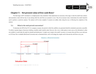
- 1. Modelling Innovation – CHAPTER 5 Free Cash Flow The Weighted Net Present (FCF) TV Estimation Average Cost of Value of Free Capital (WACC) Cash-Flows Chapter 5 - Net present value of free cash-flows1 The final stage in DCF calculation is a straight present value calculation. Some adjustments are necessary at this stage to make the model more realistic, and essentially to deal with the time of year during which the cash flows are assumed to occur. Once the net present value is determined, the model should be used to perform a sensitivity analysis. The analysis will be more complete if scenarios are added, either along the way or following the completion of the analysis. 5.1 What is the mid-period convention? To determine the NPVof the FCF of a company or project, the period in which the cashflows are generated should be simulated as precisely as possible. To achieve a greater degree of precision, building a monthly model would be ideal. However, this is not a viable option in most cases as the information is either not available or would make the model too detailed and burdensome. A simple way to improve the model’s accuracy is to assume that cash flows occur mid-year, as of 30 June.This is calledthe Mid-Period Convention and, as illustrated below, and it will change the weights used to discount the cash flows every year. Diagram 1 – Mid-period Convention 2.5 years 1.5 years 0.5 years 31 December 2012 30 June 2013 30 June 2014 30 June 2015 Valuation Date 1 © 2012, Hugo Mendes Domingos and Eduardo Vera-Cruz Pinto 1
- 2. Modelling Innovation – CHAPTER 5 In this case, the Free Cash Flow corresponding to the first year of the projections, 2013, is assumed to occur on 30 June 2013, which means that the 2013 Free Cash Flow will be reverted by 6 months. If the mid-period convention werenot adopted, the 2013 Free Cash Flow would have been discounted for a full year. Overall, adopting the mid-period convention will slightly increase the DCF value. More importantly, it will result in a more accurate model. The mid-period convention and the TV (Terminal Value). The mid-period convention affects the terminal value (TV). The TV, when calculated as a growing perpetuity, is based on the TVthat is assumed to occur as of 30 June of the final year. When calculating the value using the multiples method, the cash flow is assumed to occur onthat same date, to be consistent. In the following examples, we consider a short projection period between 2013 and 2014 only. The valuation date is as of 31 December 2012. The mid-period convention: multiples method In casethe EBITDA multiple is used to determine the TV, the multiple should be applied to the EBITDA of the last year of the projection period. The resulting TV is as of 30 June of the final year of the projection period, and therefore, the respective discount rate should be applied to calculate the present value. Diagram 2 – Mid-period Convention with multiples method Half-year FCF Valuation Date Assumed financial value for the multiple on the final day of the 31 December 2012 30 June 2013 31 December 2013 30 June 2014 final year. Bring backTV to the valuation date. 2
- 3. Modelling Innovation – CHAPTER 5 The mid-period convention: perpetuity method In this case, the assumption is that the final period’s EBIT and tax occur on 30 June (for consistency). When applying the Gordon formula, the result is that the perpetuity reverts back to the previous period. This is simply an outcome of the calculation method. As a result, the growth rate should be applied to the perpetuity value that results from the Gordon formula to make sure that the perpetuity value is taken forward to the final year of the projection period. Consequently, the discount rate used to calculate the present value of the perpetuity is the same as the one used to calculate the present value of the last year of financial projections. Diagram 3 – Mid-period Convention with perpetuity method Half year FCF Valuation Date 31 December 2012 30 June 2013 31 December 2013 30 June 2014 Bring backTV to the valuation date. 5.2 Example: detailed company valuation The following is a detailed example of a company’s valuation for the purposes of illustration. In this example, the management team of AB decided to publicly express their interest in the acquisition of a company called Innovation Models (IM). A team was mandated to advise the acquirer and assist in the 3
- 4. Modelling Innovation – CHAPTER 5 negotiations, namely, on valuation matters. IM is a stable company that sells cutting-edge industrial goods (Innovation Models rubber).The analyst’s job is to prepare a DCF valuation to determine the value of IM as of31 December 2013. Given AB’s necessity to make due diligence and negotiate the transaction, this valuation date seems appropriate. Applicable to all tables below, all periods until 2012 are historical figures, hence the “H”. From 2012 onward, all periods are estimates, hence the “E”. The current date for this example is April 2013, but we are valuing only 31 December 2013 because it is considered that there are still a few months left until the closing of the accounts and the first cash flows to be considered are from 2014. The analysts sourced key financial data from public sources, and IM’s management team provided the following information and projections: Table 1–Key financial data Net Debt (EUR M) 4,000 Perpetuity Growth Rate 2% Issued Shares 700,000,000 Tax Rate 30% Target Debt Proportion 50% Table 2 - IM management team's projections Unit 2009H 2010H 2011H 2012 2013E 2014E 2015E 2016E 2017E 2018E Operational Revenues EUR M 3,863 3,975 4,083 4,225 4,369 4,544 4,771 5,105 5,463 5,845 % change % 2.9% 2.7% 3.5% 3.4% 4.0% 5.0% 7.0% 7.0% 7.0% Gross Margin EUR M 1,468 1,630 1,756 1,732 1,704 1,818 2,004 2,297 2,677 2,864 % margin % 38.0% 41.0% 43.0% 41.0% 39.0% 40.0% 42.0% 45.0% 49.0% 49.0% EBITDA EUR M 1,082 1,232 1,307 1,310 1,267 1,409 1,574 1,787 2,130 2,280 % margin % 28.0% 31.0% 32.0% 31.0% 29.0% 31.0% 33.0% 35.0% 39.0% 39.0% EBIT EUR M 788 918 988 959 909 1,045 1,241 1,429 1,803 1,929 % margin % 20.4% 23.1% 24.2% 22.7% 20.8% 23.0% 26.0% 28.0% 33.0% 33.0% Capex EUR M (386) (477) (531) (465) (524) (545) (477) (511) (437) (468) % margin % 10.0% 12.0% 13.0% 11.0% 12.0% 12.0% 10.0% 10.0% 8.0% 8.0% Change in Net Working Capital (NWC) EUR M 4 5 5 8 8 7 9 10 11 12 % change in revenues % 4.6% 4.8% 4.6% 5.6% 5.3% 4.0% 4.0% 3.0% 3.0% 3.0% 4
- 5. Modelling Innovation – CHAPTER 5 At this stage, the analyst has all the data she needs to perform the Discounted Cash Flow analysis. The Weighted Net Present Free Cash Flow TV Estimation Average Cost of Value of Free (FCF) Capital (WACC) Cash-Flows A critical view The analyst should critically examine management’s projections. Upon analysing the figures disclosed by IM’s management team, some figures make little sense considering the financial and strategic context of the company. The following table shows the analyst’s critical analysis before she applies the DCF method. 5
- 6. Modelling Innovation – CHAPTER 5 Analyst: Growing revenues in a context in Table 3–Critical analysis which the company does Unit 2009 2010 2011 2012 2013 2014 2015 2016 2017 2018 Operational Revenues not change its strategy is (OR) EUR M 3,863 3,975 4,083 4,225 4,369 4,544 4,771 5,105 5,463 5,845 % variation % 2.9% 2.7% 3.5% 3.4% 4.0% 5.0% 7.0% 7.0% 7.0% not realistic. Gross Margin (GM) EUR M 1,468 1,630 1,756 1,732 1,704 1,818 2,004 2,297 2,677 2,864 % margin % 38.0% 41.0% 43.0% 41.0% 39.0% 40.0% 42.0% 45.0% 49.0% 49.0% Analyst: Constant EBITDA EUR M 1,082 1,232 1,307 1,310 1,267 1,409 1,574 1,787 2,130 2,280 growth in Gross % margin % 28.0% 31.0% 32.0% 31.0% 29.0% 31.0% 33.0% 35.0% 39.0% 39.0% Margins and EBIT EUR M 788 918 988 959 909 1,045 1,241 1,429 1,803 1,929 decreasing CAPEX in % margin % 20.4% 23.1% 24.2% 22.7% 20.8% 23.0% 26.0% 28.0% 33.0% 33.0% percentage of Capex EUR M (386) (477) (531) (465) (524) (545) (477) (511) (437) (468) Revenues is not % revenues % 10% 12% 13% 11% 12% 12% 10% 10% 8% 8% realistic. Change in Net Working Capital (NWC) EUR M 4 5 5 8 8 7 9 10 11 12 % Revenue Change % 4.6% 4.8% 4.6% 5.6% 5.3% 4.0% 4.0% 3.0% 3.0% 3.0% Analyst: Net Working Capital growing at a rate below revenues’ growth rate is not realistic. 6
- 7. Modelling Innovation – CHAPTER 5 Adjustments to the projections Our analyst’s views have an impact on IM’s valuation. As a result, adjustments to some figures inTable 2are needed to make the DCF valuation more realistic. Revenues and Gross Margins Table 4 - Operational revenue adjustments IM's Management Team Unit 2014E 2015E 2016E 2017E 2018E Analyst: A constant Operational Revenues EUR M 4,544 4,771 5,105 5,462 5,845 growth rate in revenues is % variation % 4.0% 5.0% 7.0% 7.0% 7.0% more realistic as there is Analyst (after revision) no change in company Operational Revenues EUR M 4,500 4,635 4,774 4,917 5,065 strategy. % variation % 3.0% 3.0% 3.0% 3.0% 3.0% Table 5 - Gross margin adjustments Analyst: Taking into account that this company’s IM's Management Team Unit 2014 2015 2016 2017 2018 market is stable, this Gross Margin EUR M 1,818 2,004 2,297 2,677 2,864 projection is more realistic. % margin % 40.0% 42.0% 45.0% 49.0% 49.0% These Gross Margins were Analyst (after revision) determined using the Gross Margin EUR M 1,818 1,872 1,928 1,986 2,046 adjusted revenues in Table 4. % margin % 40.0% 40.0% 40.0% 40.0% 40.0% 7
- 8. Modelling Innovation – CHAPTER 5 EBITDA, depreciation andamortisation, CAPEX and change in NWC Table 6 - EBITDA adjustments IM's Management Team Unit 2014 2015 2016 2017 2018 EBITDA EUR M 1,409 1,574 1,787 2,130 2,280 % margin % 31.0% 33.0% 35.0% 39.0% 39.0% Analyst: Constant Analyst (after revision) margins appear more EBITDA EUR M 1,350 1,391 1,432 1,475 1,519 realistic. % margin % 30.0% 30.0% 30.0% 30.0% 30.0% Table 7 - Depreciation and amortisation adjustments IM's Management Team Unit 2014 2015 2016 2017 2018 Dep. Amort EUR M 364 334 357 328 351 Dep. Amort. % 8.0% 7.0% 7.0% 6.0% 6.0% Analyst: Constant Analyst (after revision) D&Ais more realistic. Dep. Amort EUR M 360 371 382 393 405 Dep. Amort. % 8.0% 8.0% 8.0% 8.0% 8.0% 8
- 9. Modelling Innovation – CHAPTER 5 Table 8 - CAPEX adjustments IM's Management Team Unit 2014 2015 2016 2017 2018 Capex EUR M (545) (477) (511) (437) (468) % Revenue % 12.0% 10.0% 10.0% 8.0% 8.0% Analyst (after revision) Analyst: Constant % Capex EUR M (540) (556) (573) (590) (608) of % Revenue % 12.0% 12.0% 12.0% 12.0% 12.0% revenuesappearmore realistic. Table 9 - Net Working Capital adjustments Analyst: A constant proportion of NWC IM's Management Team Unit 2014 2015 2016 2017 2018 Net Working Capital EUR M 7.0 9.1 10.0 10.7 11.5 relative to Revenues is % Change in more realistic compared Revenue % 4.0% 4.0% 3.0% 3.0% 3.0% with the management Analyst (after revision) Net Working Capital EUR M 6.6 6.8 7.0 7.2 7.4 team´s optimistic % Change in projections. Revenue % 5.0% 5.0% 5.0% 5.0% 5.0% 9
- 10. Modelling Innovation – CHAPTER 5 This marks the end of the preview for Chapter 5. You will be able to view the rest of the contents upon publication of the full e- book. Thank you for your interest. 10