SlideShare uma empresa Scribd logo
1 de 22
Ordinary Least Squares Linear Regression: Flaws, Problems and Pitfalls
LEAST squares linear regression (also known as “least squared errors regression”, “ordinary
least squares”, “OLS”, or often just “least squares”), is one of the most basic and most
commonly used prediction techniques known to humankind, with applications in fields as
diverse as statistics, finance, medicine, economics, and psychology. Unfortunately, the technique
is frequently misused and misunderstood. Part of the difficulty lies in the fact that a great number
of people using least squares have just enough training to be able to apply it, but not enough to
training to see why it often shouldn’t be applied. What’s more, for some reason it is not very
easy to find websites that provide a critique or detailed criticism of least squares and explain
what can go wrong when you attempt to use it.
A Brief Introduction to Regression
The basic framework for regression (also known as multivariate regression, when we have
multiple independent variables involved) is the following. We have some dependent variable y
(sometimes called the output variable, label, value, or explained variable) that we would like to
predict or understand. This variable could represent, for example, people’s height in inches. We
also have some independent variables x1, x2, …, xn (sometimes called features, input variables,
predictors, or explanatory variables) that we are going to be using to make predictions for y. If
we have just two of these variables x1 and x2, they might represent, for example, people’s age
(in years), and weight (in pounds). We sometimes say that n, the number of independent
variables we are working with, is the dimension of our “feature space”, because we can think of
a particular set of values for x1, x2, …, xn as being a point in n dimensional space (with each
axis of the space formed by one independent variable). Regression is the general task of
attempting to predict values of the dependent variable y from the independent variables x1, x2,
…, xn, which in our example would be the task of predicting people’s heights using only their
ages and weights. The way that this procedure is carried out is by analyzing a set of “training”
data, which consists of samples of values of the independent variables together with
corresponding values for the dependent variables. So in our example, our training set may consist
of the weight, age, and height for a handful of people. The regression algorithm would “learn”
from this data, so that when given a “testing” set of the weight and age for people the algorithm
had never had access to before, it could predict their heights. What distinguishes regression from
other machine learning problems such as classification or ranking, is that in regression problems
the dependent variable that we are attempting to predict is a real number (as oppose to, say, an
integer or label). What’s more, in regression, when you produce a prediction that is close to the
actual true value it is considered a better answer than a prediction that is far from the true value.
Hence, if we were attempting to predict people’s heights using their weights and ages, that would
be a regression task (since height is a real number, and since in such a scenario misestimating
someone’s height by a small amount is generally better than doing so by a large amount). On the
other hand, if we were attempting to categorize each person into three groups, “short”,
“medium”, or “tall” by using only their weight and age, that would be a classification task.
Finally, if we were attempting to rank people in height order, based on their weights and ages
that would be a ranking task.
Linear Regression
Linear regression methods attempt to solve the regression problem by making the assumption
that the dependent variable is (at least to some approximation) a linear function of the
independent variables, which is the same as saying that we can estimate y using the formula:
y = c0 + c1 x1 + c2 x2 + c3 x3 + … + cn xn
where c0, c1, c2, …, cn. are some constants (i.e. fixed numbers, also known as coefficients, that
must be determined by the regression algorithm). The goal of linear regression methods is to find
the “best” choices of values for the constants c0, c1, c2, …, cn to make the formula as “accurate”
as possible (the discussion of what we mean by “best” and “accurate”, will be deferred until
later). The reason that we say this is a “linear” model is because when, for fixed constants c0 and
c1, we plot the function y(x1) (by which we mean y, thought of as a function of the independent
variable x1) which is given by
y(x1) = c0 + c1 x1
it forms a line, as in the example of the plot of y(x1) = 2 + 3 x1 below.
Likewise, if we plot the function of two variables, y(x1,x2) given by
y(x1,x2) = c0 + c1 x1 + c2 x2
it forms a plane, which is a generalization of a line. This can be seen in the plot of the example
y(x1,x2) = 2 + 3 x1 – 2 x2 below.

As we go from two independent variables to three or more, linear functions will go from forming
planes to forming hyperplanes, which are further generalizations of lines to higher dimensional
feature spaces. These hyperplanes cannot be plotted for us to see since n-dimensional planes are
displayed by embedding them in n+1 dimensional space, and our eyes and brains cannot grapple
with the four dimensional images that would be needed to draw 3 dimension hyperplanes.
However, like ordinary planes, hyperplanes can still be thought of as infinite sheets that extend
forever, and which rise (or fall) at a steady rate as we travel along them in any fixed direction.
Now, we recall that the goal of linear regression is to find choices for the constants c0, c1, c2, …,
cn that make the model y = c0 + c1 x1 + c2 x2 + c3 x3 + …. + cn xn as accurate as possible.
Values for the constants are chosen by examining past example values of the independent
variables x1, x2, x3, …, xn and the corresponding values for the dependent variable y. To return
to our height prediction example, we assume that our training data set consists of information
about a handful of people, including their weights (in pounds), ages (in years), and heights (in
inches). The idea is that perhaps we can use this training data to figure out reasonable choices for
c0, c1, c2, …, cn such that later on, when we know someone’s weight, and age but don’t know
their height, we can predict it using the (approximate) formula:
height = c0 + c1*weight + c2*age.
Least Squares Regression
As we have said, it is desirable to choose the constants c0, c1, c2, …, cn so that our linear
formula is as accurate a predictor of height as possible. But what do we mean by “accurate”? By
far the most common form of linear regression used is least squares regression (the main topic of
this essay), which provides us with a specific way of measuring “accuracy” and hence gives a
rule for how precisely to choose our “best” constants c0, c1, c2, …, cn once we are given a set of
training data (which is, in fact, the data that we will measure our accuracy on). The Least squares
method says that we are to choose these constants so that for every example point in our training
data we minimize the sum of the squared differences between the actual dependent variable and
our predicted value for the dependent variable. In other words, we want to select c0, c1, c2, …,
cn to minimize the sum of the values (actual y – predicted y)^2 for each training point, which is
the same as minimizing the sum of the values
(y – (c0 + c1 x1 + c2 x2 + c3 x3 + … + cn xn))^2
for each training point of the form (x1, x2, x3, …, y). To make this process clearer, let us return
to the example where we are predicting heights and let us apply least squares to a specific data
set. Suppose that our training data consists of (weight, age, height) data for 7 people (which, in
practice, is a very small amount of data). For example, we might have:
Person 1: (160 pounds, 19 years old, 66 inches)
Person 2: (172 pounds, 26 years old, 69 inches)
Person 3: (178 pounds, 23 years old, 72 inches)
Person 4: (170 pounds, 70 years old, 69 inches)
Person 5: (140 pounds, 15 years old, 68 inches)
Person 6: (169 pounds, 60 years old, 67 inches)
Person 7: (210 pounds, 41 years old, 73 inches)
This training data can be visualized, as in the image below, by plotting each training point in a
three dimensional space, where one axis corresponds to height, another to weight, and the third
to age:
As we have said, the least squares method attempts to minimize the sum of the squared error
between the values of the dependent variables in our training set, and our model’s predictions for
these values. Hence, in this case it is looking for the constants c0, c1 and c2 to minimize:
Sum of Squared Errors
= (66 – (c0 + c1*160 + c2*19))^2 + (69 – (c0 + c1*172 + c2*26))^2 + (72 – (c0 + c1*178 +
c2*23))^2 + (69 – (c0 + c1*170 + c2*70))^2 + (68 – (c0 + c1*140 + c2*15))^2 + (67 – (c0 +
c1*169 + c2*60))^2 + (73 – (c0 + c1*210 + c2*41))^2
The solution to this minimization problem happens to be given by
c0 = 52.8233 (inches)
c1 = 0.101546 (inches per pound)
c2 = -0.0295932 (inches per year)
Sum of Squared Errors = 14.1469
which means then that we can attempt to estimate a person’s height from their age and weight
using the following formula:
height = 52.8233 – 0.0295932 age + 0.101546 weight.
In practice however, this formula will do quite a bad job of predicting heights, and in fact
illustrates some of the problems with the way that least squares regression is often applied in
practice (as will be discussed in detail later on in this essay).
This solution for c0, c1, and c2 (which can be thought of as the plane 52.8233 – 0.0295932 x1 +
0.101546 x2) can be visualized as:
That means that for a given weight and age we can attempt to estimate a person’s height by
simply looking at the “height” of the plane for their weight and age.
Why Is Least Squares So Popular?
We’ve now seen that least squared regression provides us with a method for measuring
“accuracy” (i.e. the sum of squared errors) and that is what makes it different from other forms
of linear regression. However, least squares is such an extraordinarily popular technique that
often when people use the phrase “linear regression” they are in fact referring to “least squares
regression”. But why should people think that least squares regression is the “right” kind of
linear regression? And more generally, why do people believe that linear regression (as opposed
to non-linear regression) is the best choice of regression to begin with? Unfortunately, the
popularity of least squares regression is, in large part, driven by a series of factors that have little
to do with the question of what technique actually makes the most useful predictions in practice.
Much of the use of least squares can be attributed to the following factors:
(a) It was invented by Carl Friedrich Gauss (one of the world’s most famous mathematicians) in
about 1795, and then rediscovered by Adrien-Marie Legendre (another famous mathematician)
in 1805, making it one of the earliest general prediction methods known to humankind.
(b) It is easy to implement on a computer using commonly available algorithms from linear
algebra.
(c) Its implementation on modern computers is efficient, so it can be very quickly applied even
to problems with hundreds of features and tens of thousands of data points.
(d) It is easier to analyze mathematically than many other regression techniques.
(e) It is not too difficult for non-mathematicians to understand at a basic level.
(f) It produces solutions that are easily interpretable (i.e. we can interpret the constants that least
squares regression solves for).
(g) It is the optimal technique in a certain sense in certain special cases. In particular, if the
system being studied truly is linear with additive uncorrelated normally distributed noise (of
mean zero and constant variance) then the constants solved for by least squares are in fact the
most likely coefficients to have been used to generate the data. There is also the Gauss-Markov
theorem which states that if the underlying system we are modeling is linear with additive noise,
and the random variables representing the errors made by our ordinary least squares model are
uncorrelated from each other, and if the distributions of these random variables all have the same
variance and a mean of zero, then the least squares method is the best unbiased linear estimator
of the model coefficients (though not necessarily the best biased estimator) in that the
coefficients it leads to have the smallest variance.
While some of these justifications for using least squares are compelling under certain
circumstances, our ultimate goal should be to find the model that does the best job at making
predictions given our problem’s formulation and constraints (such as limited training points,
processing time, prediction time, and computer memory).
Problems and Pitfalls of Applying Least Squares Regression
Unfortunately, as has been mentioned above, the pitfalls of applying least squares are not
sufficiently well understood by many of the people who attempt to apply it. What follows is a list
of some of the biggest problems with using least squares regression in practice, along with some
brief comments about how these problems may be mitigated or avoided:
1. Outliers
Least squares regression can perform very badly when some points in the training data have
excessively large or small values for the dependent variable compared to the rest of the training
data. The reason for this is that since the least squares method is concerned with minimizing the
sum of the squared error, any training point that has a dependent value that differs a lot from the
rest of the data will have a disproportionately large effect on the resulting constants that are
being solved for. To further illuminate this concept, lets go back again to our example of
predicting height. Due to the squaring effect of least squares, a person in our training set whose
height is mispredicted by four inches will contribute sixteen times more error to the summed of
squared errors that is being minimized than someone whose height is mispredicted by one inch.
That means that the more abnormal a training point’s dependent value is, the more it will alter
the least squares solution. Hence a single very bad outlier can wreak havoc on prediction
accuracy by dramatically shifting the solution. If the outlier is sufficiently bad, the value of all
the points besides the outlier will be almost completely ignored merely so that the outlier’s value
can be predicted accurately. In the images below you can see the effect of adding a single outlier
(a 10 foot tall 40 year old who weights 200 pounds) to our old training set from earlier on.
Here we see a plot of our old training data set (in purple) together with our new outlier point (in
green):

Below we have a plot of the old least squares solution (in blue) prior to adding the outlier point
to our training set, and the new least squares solution (in green) which is attained after the outlier
is added:
As you can see in the image above, the outlier we added dramatically distorts the least squares
solution and hence will lead to much less accurate predictions.
The problem of outliers does not just haunt least squares regression, but also many other types of
regression (both linear and non-linear) as well. One partial solution to this problem is to measure
accuracy in a way that does not square errors. For example, the least absolute errors method
(a.k.a. least absolute deviations, which can be implemented, for example, using linear
programming or the iteratively weighted least squares technique) will emphasize outliers far less
than least squares does, and therefore can lead to much more robust predictions when extreme
outliers are present. An even more outlier robust linear regression technique is least median of
squares, which is only concerned with the median error made on the training data, not each and
every error. Unfortunately, this technique is generally less time efficient than least squares and
even than least absolute deviations.
Another solution to mitigate these problems is to preprocess the data with an outlier detection
algorithm that attempts either to remove outliers altogether or de-emphasize them by giving them
less weight than other points when constructing the linear regression model. Though sometimes
very useful, these outlier detection algorithms unfortunately have the potential to bias the
resulting model if they accidently remove or de-emphasize the wrong points. Regression
methods that attempt to model data on a local level (like local linear regression) rather than on a
global one (like ordinary least squares, where every point in the training data effects every point
in the resulting shape of the solution curve) can often be more robust to outliers in the sense that
the outliers will only distrupt the model in a small region rather than disrupting the entire model.
It should be noted that bad outliers can sometimes lead to excessively large regression constants,
and hence techniques like ridge regression and lasso regression (which dampen the size of these
constants) may perform better than least squares when outliers are present.
One thing to note about outliers is that although we have limited our discussion here to abnormal
values in the dependent variable, unusual values in the features of a point can also cause severe
problems for some regression methods, especially linear ones such as least squares. The trouble
is that if a point lies very far from the other points in feature space, then a linear model (which by
nature attributes a constant amount of change in the dependent variable for each movement of
one unit in any direction) may need to be very flat (have constant coefficients close to zero) in
order to avoid overshooting the far away point by an enormous amount. Hence, points that are
outliers in the independent variables can have a dramatic effect on the final solution, at the
expense of achieving a lot of accuracy for most of the other points.
2. Non-Linearities
All linear regression methods (including, of course, least squares regression), suffer from the
major drawback that in reality most systems are not linear. As we have discussed, linear models
attempt to fit a line through one dimensional data sets, a plane through two dimensional data sets,
and a generalization of a plane (i.e. a hyperplane) through higher dimensional data sets. In
practice though, real world relationships tend to be more complicated than simple lines or planes,
meaning that even with an infinite number of training points (and hence perfect information
about what the optimal choice of plane is) linear methods will often fail to do a good job at
making predictions. For example, trying to fit the curve y = 1-x^2 by training a linear regression
model on x and y samples taken from this function will lead to disastrous results, as is shown in
the image below. The line depicted is the least squares solution line, and the points are values of
1-x^2 for random choices of x taken from the interval [-1,1].
Notice that the least squares solution line does a terrible job of modeling the training points. In
this problem, when a very large numbers of training data points are given, a least squares
regression model (and almost any other linear model as well) will end up predicting that y is
always approximately zero. Sometimes 1-x^2 is above zero, and sometimes it is below zero, but
on average there is no tendency for 1-x^2 to increase or decrease as x increases, which is what
linear models capture. Examples like this one should remind us of the saying, “attempting to
divide the world into linear and non-linear problems is like trying to dividing organisms into
chickens and non-chickens”.
When you have a strong understanding of the system you are attempting to study, occasionally
the problem of non-linearity can be circumvented by first transforming your data in such away
that it becomes linear (for example, by applying logarithms or some other function to the
appropriate independent or dependent variables). In practice though, knowledge of what
transformations to apply in order to make a system linear is typically not available. Furthermore,
while transformations of independent variables is usually okay, transformations of the dependent
variable will cause distortions in the manner that the regression model measures errors, hence
producing what are often undesirable results.
Another possibility, if you precisely know the (non-linear) model that describes your data but
aren’t sure about the values of some parameters of this model, is to attempt to directly solve for
the optimal choice of these parameters that minimizes some notion of prediction error (or,
equivalently, maximizes some measure of accuracy). This is sometimes known as parametric
modeling, as opposed to the non-parametric modeling which will be discussed below. To give an
example, if we somehow knew that y = 2^(c0*x) + c1 x + c2 log(x) was a good model for our
system, then we could try to calculate a good choice for the constants c0, c1 and c2 using our
training data (essentially by finding the constants for which the model produces the least error on
the training data points). There are a variety of ways to do this, for example using a maximal
likelihood method or using the stochastic gradient descent method. Much of the time though, you
won’t have a good sense of what form a model describing the data might take, so this technique
will not be applicable.
Another method for avoiding the linearity problem is to apply a non-parametric regression
method such as local linear regression (a.k.a. local least squares or locally weighted scatterplot
smoothing, which can work very well when you have lots of training data and only relatively
small amounts of noise in your data) or a kernel regression technique (like the Nadaraya-Watson
method). Both of these approaches can model very complicated systems, requiring only that
some weak assumptions are met (such as that the system under consideration can be accurately
modeled by a smooth function). These non-parametric algorithms usually involve setting a
model parameter (such as a smoothing constant for local linear regression or a bandwidth
constant for kernel regression) which can be estimated using a technique like cross validation. A
troublesome aspect of these approaches is that they require being able to quickly identify all of
the training data points that are “close to” any given data point (with respect to some notion of
distance between points), which becomes very time consuming in high dimensional feature
spaces (i.e. when there are a large number of independent variables). Even worse, when we have
many independent variables in our model, the performance of these methods can rapidly erode.
Yet another possible solution to the problem of non-linearities is to apply transformations to the
independent variables of the data (prior to fitting a linear model) that map these variables into a
higher dimension space. If the transformation is chosen properly, then even if the original data is
not well modeled by a linear function, the transformed data will be. A very simple and naive use
of this procedure applied to the height prediction problem (discussed previously) would be to
take our two independent variables (weight and age) and transform them into a set of five
independent variables (weight, age, weight*age, weight^2 and age^2), which brings us from a
two dimensional feature space to a five dimensional one. Our model would then take the form:
height = c0 + c1*weight + c2*age + c3*weight*age + c4*weight^2 + c5*age^2
This new model is linear in the new (transformed) feature space (weight, age, weight*age,
weight^2 and age^2), but is non-linear in the original feature space (weight, age). The procedure
used in this example is very ad hoc however and does not represent how one should generally
select these feature transformations in practice (unless a priori knowledge tells us that this
transformed set of features would be an adequate choice). To automate such a procedure, the
Kernel Principle Component Analysis technique and other so called Nonlinear Dimensionality
Reduction techniques can automatically transform the input data (non-linearly) into a new
feature space that is chosen to capture important characteristics of the data. When a linear model
is applied to the new independent variables produced by these methods, it leads to a non-linear
model in the space of the original independent variables.
A related (and often very, very good) solution to the non-linearity problem is to directly apply a
so-called “kernel method” like support vector regression or kernelized ridge regression (a.k.a.
kernelized Tikhonov regularization) with an appropriate choice of a non-linear kernel function.
These methods automatically apply linear regression in a non-linearly transformed version of
your feature space (with the actual transformation used determined by the choice of kernel
function) which produces non-linear models in the original feature space. Certain choices of
kernel function, like the Gaussian kernel (sometimes called a radial basis function kernel or RBF
kernel), will lead to models that are consistent, meaning that they can fit virtually any system to
arbitrarily good accuracy, so long as a sufficiently large amount of training data points are
available. All regular linear regression algorithms conspicuously lack this very desirable
property.
It should be noted that when the number of input variables is very large, the restriction of using a
linear model may not be such a bad one (because the set of planes in a very large dimensional
space may actually be quite a flexible model). Furthermore, when we are dealing with very noisy
data sets and a small numbers of training points, sometimes a non-linear model is too much to
ask for in a sense because we don’t have enough data to justify a model of large complexity (and
if only very simple models are possible to use, a linear model is often a reasonable choice). That
being said (as shall be discussed below) least squares regression generally performs very badly
when there are too few training points compared to the number of independent variables, so even
scenarios with small amounts of training data often do not justify the use of least squares
regression. These scenarios may, however, justify other forms of linear regression. An important
idea to be aware of is that it is typically better to apply a method that will automatically
determine how much complexity can be afforded when fitting a set of training data than to apply
an overly simplistic linear model that always uses the same level of complexity (which may, in
some cases be too much, and overfit the data, and in other cases be too little, and underfit it).
When the support vector regression technique and ridge regression technique use linear kernel
functions (and hence are performing a type of linear regression) they generally avoid overfitting
by automatically tuning their own levels of complexity, but even so cannot generally avoid
underfitting (since linear models just aren’t complex enough to model some systems accurately
when given a fixed set of features). The kernelized (i.e. non-linear) versions of these techniques,
however, can avoid both overfitting and underfitting since they are not restricted to a simplistic
linear model.
3. Too Many Variables
While intuitively it seems as though the more information we have about a system the easier it is
to make predictions about it, with many (if not most) commonly used algorithms the opposite
can occasionally turn out to be the case. While it never hurts to have a large amount of training
data (except insofar as it will generally slow down the training process), having too many
features (i.e. independent variables) can cause serious difficulties. Least squares regression is
particularly prone to this problem, for as soon as the number of features used exceeds the number
of training data points, the least squares solution will not be unique, and hence the least squares
algorithm will fail. In practice, as we add a large number of independent variables to our least
squares model, the performance of the method will typically erode before this critical point
(where the number of features begins to exceed the number of training points) is reached. This
implies that rather than just throwing every independent variable we have access to into our
regression model, it can be beneficial to only include those features that are likely to be good
predictors of our output variable (especially when the number of training points available isn’t
much bigger than the number of possible features). What’s more, we should avoid including
redundant information in our features because they are unlikely to help, and (since they increase
the total number of features) may impair the regression algorithm’s ability to make accurate
predictions. Keep in mind that when a large number of features is used, it may take a lot of
training points to accurately distinguish between those features that are correlated with the output
variable just by chance, and those which meaningfully relate to it. Some regression methods (like
least squares) are much more prone to this problem than others.
As the number of independent variables in a regression model increases, its R^2 (which
measures what fraction of the variability (variance) in the training data that the prediction
method is able to account for) will always go up. This increase in R^2 may lead some
inexperienced practitioners to think that the model has gotten better. When applying least squares
regression, however, it is not the R^2 on the training data that is significant, but rather the R^2
that the model will achieve on the data that we are interested in making prediction for (i.e. we
care about error on the test set, not the training set). When too many variables are used with the
least squares method the model begins finding ways to fit itself to not only the underlying
structure of the training set, but to the noise in the training set as well, which is one way to
explain why too many features leads to bad prediction results.
One way to help solve the problem of too many independent variables is to scrutinize all of the
possible independent variables, and discard all but a few (keeping a subset of those that are very
useful in predicting the dependent variable, but aren’t too similar to each other). For least squares
regression, the number of independent variables chosen should be much smaller than the size of
the training set. This approach can be carried out systematically by applying a feature selection
or dimensionality reduction algorithm (such as subset selection, principal component analysis,
kernel principal component analysis, or independent component analysis) to preprocess the data
and automatically boil down a large number of input variables into a much smaller number.
Some of these methods automatically remove many of the features, whereas others combine
features together into a smaller number of new features. These algorithms can be very useful in
practice, but occasionally will eliminate or reduce the importance of features that are very
important, leading to bad predictions. It is crtitical that, before certain of these feature selection
methods are applied, the independent variables are normalized so that they have comparable
units (which is often done by setting the mean of each feature to zero, and the standard deviation
of each feature to one, by use of subtraction and then division).
Another approach to solving the problem of having a large number of possible variables is to use
lasso linear regression which does a good job of automatically eliminating the effect of some
independent variables. Other regression techniques that can perform very well when there are
very large numbers of features (including cases where the number of independent variables
exceeds the number of training points) are support vector regression, ridge regression, and partial
least squares regression.
4. Dependence Among Variables
The least squares method can sometimes lead to poor predictions when a subset of the
independent variables fed to it are significantly correlated to each other. The problem in these
circumstances is that there are a variety of different solutions to the regression problem that the
model considers to be almost equally good (as far as the training data is concerned), but
unfortunately many of these “nearly equal” solutions will lead to very bad predictions (i.e. poor
performance on the testing set). To illustrate this point, lets take the extreme example where we
use the same independent variable twice with different names (and hence have two input
variables that are perfectly correlated to each other). If these perfectly correlated independent
variables are called w1 and w2, then we note that our least squares regression algorithm doesn’t
distinguish between the two solutions
y = .5*w1 + .5*w2
and
y = 1000*w1 – 999*w2
since
.5*w1 + .5*w2 = .5*w1 + .5*w1 = w1
and
1000*w1 – 999*w2 = 1000*w1 – 999*w1 = w1.
In both cases the models tell us that y tends to go up on average about one unit when w1 goes up
one unit (since we can simply think of w2 as being replaced with w1 in these equations, as was
done above). Intuitively though, the second model is likely much worse than the first, because if
w2 ever begins to deviate even slightly from w1 the predictions of the second model will change
dramatically. For example, if for a single prediction point w2 were equal to .95 w1 rather than
the precisely one w1 that we expected, then we would find that the first model would give the
prediction
y = .5*w1 + .5*w2 = .5*w1 + .5*0.95*w1 = 0.975 w1
which is very close to the prediction of simply one w1 that we get without this change in w2. On
the other hand, in these circumstances the second model would give the prediction
y = 1000*w1 – 999*w2 = 1000*w1 – 999*0.95*w1 = 50.95 w1
which isn’t even close to our old prediction of just one w1. Hence we see that dependencies in
our independent variables can lead to very large constant coefficients in least squares regression,
which produce predictions that swing wildly and insanely if the relationships that held in the
training set (perhaps, only by chance) do not hold precisely for the points that we are attempting
to make predictions on.
A common solution to this problem is to apply ridge regression or lasso regression rather than
least squares regression. Both of these methods have the helpful advantage that they try to avoid
producing models that have large coefficients, and hence often perform much better when strong
dependencies are present. It should be noted that when the number of training points is
sufficiently large (for the given number of features in the problem and the distribution of noise)
correlations among the features may not be at all problematic for the least squares method. On
the other hand though, when the number of training points is insufficient, strong correlations can
lead to very bad results.
5. Wrong Choice of Error Function
As we have said before, least squares regression attempts to minimize the sum of the squared
differences between the values predicted by the model and the values actually observed in the
training data. More formally, least squares regression is trying to find the constant coefficients
c1, c2, c3, …, cn to minimize the quantity
(y – (c1 x1 + c2 x2+ c3 x3 + … + cn xn))^2
when it is summed over each of the different training points (i.e. different know values for y, x1,
x2, x3, …, xn).
But why is it the sum of the squared errors that we are interested in? Is mispredicting one
person’s height by two inches really as equally “bad” as mispredicting four people’s height by 1
inch each, as least squares regression implicitly assumes? Should mispredicting one person’s
height by 4 inches really be precisely sixteen times “worse” than mispredicting one person’s
height by 1 inch? This (not necessarily desirable) result is a consequence of the method for
measuring error that least squares employs. In general we would rather have a small sum of
squared errors rather than a large one (all else being equal), but that does not mean that the sum
of squared errors is the best measure of error for us to try and minimize. The simple conclusion
is that the way that least squares regression measures error is often not justified.
Lets use a simplistic and artificial example to illustrate this point. Suppose that we are in the
insurance business and have to predict when it is that people will die so that we can appropriately
value their insurance policies. Furthermore, suppose that when we incorrectly identify the year
when a person will die, our company will be exposed to losing an amount of money that is
proportional to the absolute value of the error in our prediction. In other words, if we predict that
someone will die in 1993, but they actually die in 1994, we will lose half as much money as if
they died in 1995, since in the latter case our estimate was off by twice as many years as in the
former case. What’s more, in this scenario, missing someone’s year of death by two years is
precisely as bad to us as mispredicting two people’s years of death by one year each (since the
same number of dollars will be lost by us in both cases). If we are concerned with losing as little
money as possible, then it is is clear that the right notion of error to minimize in our model is the
sum of the absolute value of the errors in our predictions (since this quantity will be proportional
to the total money lost), not the sum of the squared errors in predictions that least squares uses.
In some many cases we won’t know exactly what measure of error is best to minimize, but we
may be able to determine that some choices are better than others. The point is, if you are
interested in doing a good job to solve the problem that you have at hand, you shouldn’t just
blindly apply least squares, but rather should see if you can find a better way of measuring error
(than the sum of squared errors) that is more appropriate to your problem. Sum of squared error
minimization is very popular because the equations involved tend to work out nice
mathematically (often as matrix equations) leading to algorithms that are easy to analyze and
implement on computers. But frequently this does not provide the best way of measuring errors
for a given problem.
It should be noted that there are certain special cases when minimizing the sum of squared errors
is justified due to theoretical considerations. One such justification comes from the relationship
between the sum of squares and the arithmetic mean (usually just called “the mean”). Suppose
that we have samples from a function that we are attempting to fit, where noise has been added
to the values of the dependent variable, and the distribution of noise added at each point may
depend on the location of that point in feature space. In that case, if we have a (parametric)
model that we know encompasses the true function from which the samples were drawn, then
solving for the model coefficients by minimizing the sum of squared errors will lead to an
estimate of the true function’s mean value at each point. On the other hand, if we instead
minimize the sum of the absolute value of the errors, this will produce estimates of the median of
the true function at each point. Hence, in cases such as this one, our choice of error function will
ultimately determine the quantity we are estimating (function(x) + mean(noise(x)), function(x) +
median(noise(x)), or what have you). Since the mean has some desirable properties and, in
particular, since the noise term is sometimes known to have a mean of zero, exceptional
situations like this one can occasionally justify the minimization of the sum of squared errors
rather than of other error functions.
6. Unequal Training Point Variances (Heteroskedasticity)
Interestingly enough, even if the underlying system that we are attempting to model truly is
linear, and even if (for the task at hand) the best way of measuring error truly is the sum of
squared errors, and even if we have plenty of training data compared to the number of
independent variables in our model, and even if our training data does not have significant
outliers or dependence between independent variables, it is STILL not necessarily the case that
least squares (in its usual form) is the optimal model to use. The difficulty is that the level of
noise in our data may be dependent on what region of our feature space we are in. For example,
going back to our height prediction scenario, there may be more variation in the heights of
people who are ten years old than in those who are fifty years old, or there more be more
variation in the heights of people who weight 100 pounds than in those who weight 200 pounds.
The upshot of this is that some points in our training data are more likely to be effected by noise
than some other such points, which means that some points in our training set are more reliable
than others. We don’t want to ignore the less reliable points completely (since that would be
wasting valuable information) but they should count less in our computation of the optimal
constants c0, c1, c2, …, cn than points that come from regions of space with less noise. To do
this one can use the technique known as weighted least squares which puts more “weight” on
more reliable points. In practice though, since the amount of noise at each point in feature space
is typically not known, approximate methods (such as feasible generalized least squares) which
attempt to estimate the optimal weight for each training point are used.
7. Wrong Choice of Features
The problem of selecting the wrong independent variables (i.e. features) for a prediction problem
is one that plagues all regression methods, not just least squares regression. To illustrate this
problem in its simplest form, suppose that our goal is to predict people’s IQ scores, and the
features that we are using to make our predictions are the average number of hours that each
person sleeps at night and the number of children that each person has. Clearly, using these
features the prediction problem is essentially impossible because their is so little relationship (if
any at all) between the independent variables and the dependent variable. No model or learning
algorithm no matter how good is going to rectify this situation. What’s worse, if we have very
limited amounts of training data to build our model from, then our regression algorithm may
even discover spurious relationships between the independent variables and dependent variable
that only happen to be there due to chance (i.e. random fluctuation). Even if many of our features
are in fact good ones, the genuine relations between the independent variables the dependent
variable may well be overwhelmed by the effect of many poorly selected features that add noise
to the learning process. When carrying out any form of regression, it is extremely important to
carefully select the features that will be used by the regression algorithm, including those
features that are likely to have a strong effect on the dependent variable, and excluding those that
are unlikely to have much effect.
8. Noise in the Independent Variables
While least squares regression is designed to handle noise in the dependent variable, the same is
not the case with noise (errors) in the independent variables. Noise in the features can arise for a
variety of reasons depending on the context, including measurement error, transcription error (if
data was entered by hand or scanned into a computer), rounding error, or inherent uncertainty in
the system being studied. Models that specifically attempt to handle cases such as these are
sometimes known as errors in variables models. When a substantial amount of noise in the
independent variables is present, the total least squares technique (which measures error using
the distance between training points and the prediction plane, rather than the difference between
the training point dependent variables and the predicted values for these variables) may be more
appropriate than ordinary least squares. Another option is to employ least products regression.
Conclusion
Although least squares regression is undoubtedly a useful and important technique, it has many
defects, and is often not the best method to apply in real world situations. A great deal of subtlety
is involved in finding the best solution to a given prediction problem, and it is important to be
aware of all the things that can go wrong.

Mais conteúdo relacionado

Mais procurados

Simple linear regression (final)
Simple linear regression (final)Simple linear regression (final)
Simple linear regression (final)
Harsh Upadhyay
 

Mais procurados (20)

Linear regression
Linear regressionLinear regression
Linear regression
 
Multiple linear regression
Multiple linear regressionMultiple linear regression
Multiple linear regression
 
Ols
OlsOls
Ols
 
Heteroscedasticity
HeteroscedasticityHeteroscedasticity
Heteroscedasticity
 
Regression analysis
Regression analysisRegression analysis
Regression analysis
 
Autocorrelation
AutocorrelationAutocorrelation
Autocorrelation
 
7 classical assumptions of ordinary least squares
7 classical assumptions of ordinary least squares7 classical assumptions of ordinary least squares
7 classical assumptions of ordinary least squares
 
Multicollinearity PPT
Multicollinearity PPTMulticollinearity PPT
Multicollinearity PPT
 
Introduction to R
Introduction to RIntroduction to R
Introduction to R
 
Least Squares Regression Method | Edureka
Least Squares Regression Method | EdurekaLeast Squares Regression Method | Edureka
Least Squares Regression Method | Edureka
 
Time series Analysis
Time series AnalysisTime series Analysis
Time series Analysis
 
Logistic regression with SPSS
Logistic regression with SPSSLogistic regression with SPSS
Logistic regression with SPSS
 
Regression
RegressionRegression
Regression
 
Autocorrelation
AutocorrelationAutocorrelation
Autocorrelation
 
Heteroscedasticity
HeteroscedasticityHeteroscedasticity
Heteroscedasticity
 
Simple linear regression
Simple linear regressionSimple linear regression
Simple linear regression
 
Crosstabs
CrosstabsCrosstabs
Crosstabs
 
Multicolinearity
MulticolinearityMulticolinearity
Multicolinearity
 
time series analysis
time series analysistime series analysis
time series analysis
 
Simple linear regression (final)
Simple linear regression (final)Simple linear regression (final)
Simple linear regression (final)
 

Destaque

Least square method
Least square methodLeast square method
Least square method
Somya Bagai
 
The least square method
The least square methodThe least square method
The least square method
kevinlefol
 
Regression analysis ppt
Regression analysis pptRegression analysis ppt
Regression analysis ppt
Elkana Rorio
 
Method of least square
Method of least squareMethod of least square
Method of least square
Somya Bagai
 
STATA - Introduction
STATA - IntroductionSTATA - Introduction
STATA - Introduction
stata_org_uk
 
Regression analysis
Regression analysisRegression analysis
Regression analysis
saba khan
 
ORDINARY LEAST SQUARES REGRESSION OF ORDERED CATEGORICAL DATA- IN
ORDINARY LEAST SQUARES REGRESSION OF ORDERED CATEGORICAL DATA- INORDINARY LEAST SQUARES REGRESSION OF ORDERED CATEGORICAL DATA- IN
ORDINARY LEAST SQUARES REGRESSION OF ORDERED CATEGORICAL DATA- IN
Beth Larrabee
 
Stats powerpoint presentation
Stats powerpoint presentationStats powerpoint presentation
Stats powerpoint presentation
jpratt23
 
A&S 350 Vr
A&S 350 VrA&S 350 Vr
A&S 350 Vr
zjmo222
 
L2 flash cards quantitative methods - SS3
L2 flash cards quantitative methods - SS3L2 flash cards quantitative methods - SS3
L2 flash cards quantitative methods - SS3
analystbuddy
 

Destaque (20)

Least square method
Least square methodLeast square method
Least square method
 
The least square method
The least square methodThe least square method
The least square method
 
Regression analysis ppt
Regression analysis pptRegression analysis ppt
Regression analysis ppt
 
METHOD OF LEAST SQURE
METHOD OF LEAST SQUREMETHOD OF LEAST SQURE
METHOD OF LEAST SQURE
 
Method of least square
Method of least squareMethod of least square
Method of least square
 
Regression
RegressionRegression
Regression
 
Lecture 4
Lecture 4Lecture 4
Lecture 4
 
Data Science - Part IV - Regression Analysis & ANOVA
Data Science - Part IV - Regression Analysis & ANOVAData Science - Part IV - Regression Analysis & ANOVA
Data Science - Part IV - Regression Analysis & ANOVA
 
STATA - Introduction
STATA - IntroductionSTATA - Introduction
STATA - Introduction
 
Simple (and Simplistic) Introduction to Econometrics and Linear Regression
Simple (and Simplistic) Introduction to Econometrics and Linear RegressionSimple (and Simplistic) Introduction to Econometrics and Linear Regression
Simple (and Simplistic) Introduction to Econometrics and Linear Regression
 
Curve fitting
Curve fitting Curve fitting
Curve fitting
 
Regression analysis
Regression analysisRegression analysis
Regression analysis
 
Regression Analysis
Regression AnalysisRegression Analysis
Regression Analysis
 
ORDINARY LEAST SQUARES REGRESSION OF ORDERED CATEGORICAL DATA- IN
ORDINARY LEAST SQUARES REGRESSION OF ORDERED CATEGORICAL DATA- INORDINARY LEAST SQUARES REGRESSION OF ORDERED CATEGORICAL DATA- IN
ORDINARY LEAST SQUARES REGRESSION OF ORDERED CATEGORICAL DATA- IN
 
Stats powerpoint presentation
Stats powerpoint presentationStats powerpoint presentation
Stats powerpoint presentation
 
A&S 350 Vr
A&S 350 VrA&S 350 Vr
A&S 350 Vr
 
Least Squares
Least SquaresLeast Squares
Least Squares
 
Econ141 s1 08
Econ141 s1 08Econ141 s1 08
Econ141 s1 08
 
L2 flash cards quantitative methods - SS3
L2 flash cards quantitative methods - SS3L2 flash cards quantitative methods - SS3
L2 flash cards quantitative methods - SS3
 
Rank correlation- some features and an application
Rank correlation- some features and an applicationRank correlation- some features and an application
Rank correlation- some features and an application
 

Semelhante a Ordinary least squares linear regression

Machine learning (11)
Machine learning (11)Machine learning (11)
Machine learning (11)
NYversity
 

Semelhante a Ordinary least squares linear regression (20)

Simple linear regression
Simple linear regressionSimple linear regression
Simple linear regression
 
Line of best fit lesson
Line of best fit lessonLine of best fit lesson
Line of best fit lesson
 
Basic statistics by_david_solomon_hadi_-_split_and_reviewed
Basic statistics by_david_solomon_hadi_-_split_and_reviewedBasic statistics by_david_solomon_hadi_-_split_and_reviewed
Basic statistics by_david_solomon_hadi_-_split_and_reviewed
 
working with python
working with pythonworking with python
working with python
 
Principal component analysis
Principal component analysisPrincipal component analysis
Principal component analysis
 
Powerpoint2.reg
Powerpoint2.regPowerpoint2.reg
Powerpoint2.reg
 
Essentials of machine learning algorithms
Essentials of machine learning algorithmsEssentials of machine learning algorithms
Essentials of machine learning algorithms
 
Machine learning (11)
Machine learning (11)Machine learning (11)
Machine learning (11)
 
REGRESSION ANALYSIS THEORY EXPLAINED HERE
REGRESSION ANALYSIS THEORY EXPLAINED HEREREGRESSION ANALYSIS THEORY EXPLAINED HERE
REGRESSION ANALYSIS THEORY EXPLAINED HERE
 
MSE.pptx
MSE.pptxMSE.pptx
MSE.pptx
 
wzhu_paper
wzhu_paperwzhu_paper
wzhu_paper
 
Basics of Stats (2).pptx
Basics of Stats (2).pptxBasics of Stats (2).pptx
Basics of Stats (2).pptx
 
Simulation notes
Simulation notesSimulation notes
Simulation notes
 
DETECTION OF MOVING OBJECT
DETECTION OF MOVING OBJECTDETECTION OF MOVING OBJECT
DETECTION OF MOVING OBJECT
 
Mathematical blog #1
Mathematical blog #1Mathematical blog #1
Mathematical blog #1
 
Practical Digital Image Processing 5
Practical Digital Image Processing 5Practical Digital Image Processing 5
Practical Digital Image Processing 5
 
Understanding Blackbox Prediction via Influence Functions
Understanding Blackbox Prediction via Influence FunctionsUnderstanding Blackbox Prediction via Influence Functions
Understanding Blackbox Prediction via Influence Functions
 
ML Module 3.pdf
ML Module 3.pdfML Module 3.pdf
ML Module 3.pdf
 
Cs229 notes10
Cs229 notes10Cs229 notes10
Cs229 notes10
 
Bootcamp of new world to taken seriously
Bootcamp of new world to taken seriouslyBootcamp of new world to taken seriously
Bootcamp of new world to taken seriously
 

Último

FULL ENJOY Call Girls In Majnu Ka Tilla, Delhi Contact Us 8377877756
FULL ENJOY Call Girls In Majnu Ka Tilla, Delhi Contact Us 8377877756FULL ENJOY Call Girls In Majnu Ka Tilla, Delhi Contact Us 8377877756
FULL ENJOY Call Girls In Majnu Ka Tilla, Delhi Contact Us 8377877756
dollysharma2066
 
Call Girls Hebbal Just Call 👗 7737669865 👗 Top Class Call Girl Service Bangalore
Call Girls Hebbal Just Call 👗 7737669865 👗 Top Class Call Girl Service BangaloreCall Girls Hebbal Just Call 👗 7737669865 👗 Top Class Call Girl Service Bangalore
Call Girls Hebbal Just Call 👗 7737669865 👗 Top Class Call Girl Service Bangalore
amitlee9823
 
Mifty kit IN Salmiya (+918133066128) Abortion pills IN Salmiyah Cytotec pills
Mifty kit IN Salmiya (+918133066128) Abortion pills IN Salmiyah Cytotec pillsMifty kit IN Salmiya (+918133066128) Abortion pills IN Salmiyah Cytotec pills
Mifty kit IN Salmiya (+918133066128) Abortion pills IN Salmiyah Cytotec pills
Abortion pills in Kuwait Cytotec pills in Kuwait
 
Call Girls Electronic City Just Call 👗 7737669865 👗 Top Class Call Girl Servi...
Call Girls Electronic City Just Call 👗 7737669865 👗 Top Class Call Girl Servi...Call Girls Electronic City Just Call 👗 7737669865 👗 Top Class Call Girl Servi...
Call Girls Electronic City Just Call 👗 7737669865 👗 Top Class Call Girl Servi...
amitlee9823
 
unwanted pregnancy Kit [+918133066128] Abortion Pills IN Dubai UAE Abudhabi
unwanted pregnancy Kit [+918133066128] Abortion Pills IN Dubai UAE Abudhabiunwanted pregnancy Kit [+918133066128] Abortion Pills IN Dubai UAE Abudhabi
unwanted pregnancy Kit [+918133066128] Abortion Pills IN Dubai UAE Abudhabi
Abortion pills in Kuwait Cytotec pills in Kuwait
 

Último (20)

FULL ENJOY Call Girls In Majnu Ka Tilla, Delhi Contact Us 8377877756
FULL ENJOY Call Girls In Majnu Ka Tilla, Delhi Contact Us 8377877756FULL ENJOY Call Girls In Majnu Ka Tilla, Delhi Contact Us 8377877756
FULL ENJOY Call Girls In Majnu Ka Tilla, Delhi Contact Us 8377877756
 
Monthly Social Media Update April 2024 pptx.pptx
Monthly Social Media Update April 2024 pptx.pptxMonthly Social Media Update April 2024 pptx.pptx
Monthly Social Media Update April 2024 pptx.pptx
 
Call Girls In Panjim North Goa 9971646499 Genuine Service
Call Girls In Panjim North Goa 9971646499 Genuine ServiceCall Girls In Panjim North Goa 9971646499 Genuine Service
Call Girls In Panjim North Goa 9971646499 Genuine Service
 
Call Girls Hebbal Just Call 👗 7737669865 👗 Top Class Call Girl Service Bangalore
Call Girls Hebbal Just Call 👗 7737669865 👗 Top Class Call Girl Service BangaloreCall Girls Hebbal Just Call 👗 7737669865 👗 Top Class Call Girl Service Bangalore
Call Girls Hebbal Just Call 👗 7737669865 👗 Top Class Call Girl Service Bangalore
 
B.COM Unit – 4 ( CORPORATE SOCIAL RESPONSIBILITY ( CSR ).pptx
B.COM Unit – 4 ( CORPORATE SOCIAL RESPONSIBILITY ( CSR ).pptxB.COM Unit – 4 ( CORPORATE SOCIAL RESPONSIBILITY ( CSR ).pptx
B.COM Unit – 4 ( CORPORATE SOCIAL RESPONSIBILITY ( CSR ).pptx
 
👉Chandigarh Call Girls 👉9878799926👉Just Call👉Chandigarh Call Girl In Chandiga...
👉Chandigarh Call Girls 👉9878799926👉Just Call👉Chandigarh Call Girl In Chandiga...👉Chandigarh Call Girls 👉9878799926👉Just Call👉Chandigarh Call Girl In Chandiga...
👉Chandigarh Call Girls 👉9878799926👉Just Call👉Chandigarh Call Girl In Chandiga...
 
Enhancing and Restoring Safety & Quality Cultures - Dave Litwiller - May 2024...
Enhancing and Restoring Safety & Quality Cultures - Dave Litwiller - May 2024...Enhancing and Restoring Safety & Quality Cultures - Dave Litwiller - May 2024...
Enhancing and Restoring Safety & Quality Cultures - Dave Litwiller - May 2024...
 
Lucknow 💋 Escorts in Lucknow - 450+ Call Girl Cash Payment 8923113531 Neha Th...
Lucknow 💋 Escorts in Lucknow - 450+ Call Girl Cash Payment 8923113531 Neha Th...Lucknow 💋 Escorts in Lucknow - 450+ Call Girl Cash Payment 8923113531 Neha Th...
Lucknow 💋 Escorts in Lucknow - 450+ Call Girl Cash Payment 8923113531 Neha Th...
 
Boost the utilization of your HCL environment by reevaluating use cases and f...
Boost the utilization of your HCL environment by reevaluating use cases and f...Boost the utilization of your HCL environment by reevaluating use cases and f...
Boost the utilization of your HCL environment by reevaluating use cases and f...
 
Mifty kit IN Salmiya (+918133066128) Abortion pills IN Salmiyah Cytotec pills
Mifty kit IN Salmiya (+918133066128) Abortion pills IN Salmiyah Cytotec pillsMifty kit IN Salmiya (+918133066128) Abortion pills IN Salmiyah Cytotec pills
Mifty kit IN Salmiya (+918133066128) Abortion pills IN Salmiyah Cytotec pills
 
Best VIP Call Girls Noida Sector 40 Call Me: 8448380779
Best VIP Call Girls Noida Sector 40 Call Me: 8448380779Best VIP Call Girls Noida Sector 40 Call Me: 8448380779
Best VIP Call Girls Noida Sector 40 Call Me: 8448380779
 
Value Proposition canvas- Customer needs and pains
Value Proposition canvas- Customer needs and painsValue Proposition canvas- Customer needs and pains
Value Proposition canvas- Customer needs and pains
 
Call Girls Electronic City Just Call 👗 7737669865 👗 Top Class Call Girl Servi...
Call Girls Electronic City Just Call 👗 7737669865 👗 Top Class Call Girl Servi...Call Girls Electronic City Just Call 👗 7737669865 👗 Top Class Call Girl Servi...
Call Girls Electronic City Just Call 👗 7737669865 👗 Top Class Call Girl Servi...
 
RSA Conference Exhibitor List 2024 - Exhibitors Data
RSA Conference Exhibitor List 2024 - Exhibitors DataRSA Conference Exhibitor List 2024 - Exhibitors Data
RSA Conference Exhibitor List 2024 - Exhibitors Data
 
John Halpern sued for sexual assault.pdf
John Halpern sued for sexual assault.pdfJohn Halpern sued for sexual assault.pdf
John Halpern sued for sexual assault.pdf
 
The Coffee Bean & Tea Leaf(CBTL), Business strategy case study
The Coffee Bean & Tea Leaf(CBTL), Business strategy case studyThe Coffee Bean & Tea Leaf(CBTL), Business strategy case study
The Coffee Bean & Tea Leaf(CBTL), Business strategy case study
 
Organizational Transformation Lead with Culture
Organizational Transformation Lead with CultureOrganizational Transformation Lead with Culture
Organizational Transformation Lead with Culture
 
VIP Call Girls In Saharaganj ( Lucknow ) 🔝 8923113531 🔝 Cash Payment (COD) 👒
VIP Call Girls In Saharaganj ( Lucknow  ) 🔝 8923113531 🔝  Cash Payment (COD) 👒VIP Call Girls In Saharaganj ( Lucknow  ) 🔝 8923113531 🔝  Cash Payment (COD) 👒
VIP Call Girls In Saharaganj ( Lucknow ) 🔝 8923113531 🔝 Cash Payment (COD) 👒
 
Ensure the security of your HCL environment by applying the Zero Trust princi...
Ensure the security of your HCL environment by applying the Zero Trust princi...Ensure the security of your HCL environment by applying the Zero Trust princi...
Ensure the security of your HCL environment by applying the Zero Trust princi...
 
unwanted pregnancy Kit [+918133066128] Abortion Pills IN Dubai UAE Abudhabi
unwanted pregnancy Kit [+918133066128] Abortion Pills IN Dubai UAE Abudhabiunwanted pregnancy Kit [+918133066128] Abortion Pills IN Dubai UAE Abudhabi
unwanted pregnancy Kit [+918133066128] Abortion Pills IN Dubai UAE Abudhabi
 

Ordinary least squares linear regression

  • 1. Ordinary Least Squares Linear Regression: Flaws, Problems and Pitfalls LEAST squares linear regression (also known as “least squared errors regression”, “ordinary least squares”, “OLS”, or often just “least squares”), is one of the most basic and most commonly used prediction techniques known to humankind, with applications in fields as diverse as statistics, finance, medicine, economics, and psychology. Unfortunately, the technique is frequently misused and misunderstood. Part of the difficulty lies in the fact that a great number of people using least squares have just enough training to be able to apply it, but not enough to training to see why it often shouldn’t be applied. What’s more, for some reason it is not very easy to find websites that provide a critique or detailed criticism of least squares and explain what can go wrong when you attempt to use it. A Brief Introduction to Regression The basic framework for regression (also known as multivariate regression, when we have multiple independent variables involved) is the following. We have some dependent variable y (sometimes called the output variable, label, value, or explained variable) that we would like to predict or understand. This variable could represent, for example, people’s height in inches. We also have some independent variables x1, x2, …, xn (sometimes called features, input variables, predictors, or explanatory variables) that we are going to be using to make predictions for y. If we have just two of these variables x1 and x2, they might represent, for example, people’s age (in years), and weight (in pounds). We sometimes say that n, the number of independent variables we are working with, is the dimension of our “feature space”, because we can think of a particular set of values for x1, x2, …, xn as being a point in n dimensional space (with each axis of the space formed by one independent variable). Regression is the general task of attempting to predict values of the dependent variable y from the independent variables x1, x2, …, xn, which in our example would be the task of predicting people’s heights using only their ages and weights. The way that this procedure is carried out is by analyzing a set of “training” data, which consists of samples of values of the independent variables together with corresponding values for the dependent variables. So in our example, our training set may consist of the weight, age, and height for a handful of people. The regression algorithm would “learn” from this data, so that when given a “testing” set of the weight and age for people the algorithm
  • 2. had never had access to before, it could predict their heights. What distinguishes regression from other machine learning problems such as classification or ranking, is that in regression problems the dependent variable that we are attempting to predict is a real number (as oppose to, say, an integer or label). What’s more, in regression, when you produce a prediction that is close to the actual true value it is considered a better answer than a prediction that is far from the true value. Hence, if we were attempting to predict people’s heights using their weights and ages, that would be a regression task (since height is a real number, and since in such a scenario misestimating someone’s height by a small amount is generally better than doing so by a large amount). On the other hand, if we were attempting to categorize each person into three groups, “short”, “medium”, or “tall” by using only their weight and age, that would be a classification task. Finally, if we were attempting to rank people in height order, based on their weights and ages that would be a ranking task. Linear Regression Linear regression methods attempt to solve the regression problem by making the assumption that the dependent variable is (at least to some approximation) a linear function of the independent variables, which is the same as saying that we can estimate y using the formula: y = c0 + c1 x1 + c2 x2 + c3 x3 + … + cn xn where c0, c1, c2, …, cn. are some constants (i.e. fixed numbers, also known as coefficients, that must be determined by the regression algorithm). The goal of linear regression methods is to find the “best” choices of values for the constants c0, c1, c2, …, cn to make the formula as “accurate” as possible (the discussion of what we mean by “best” and “accurate”, will be deferred until later). The reason that we say this is a “linear” model is because when, for fixed constants c0 and c1, we plot the function y(x1) (by which we mean y, thought of as a function of the independent variable x1) which is given by y(x1) = c0 + c1 x1 it forms a line, as in the example of the plot of y(x1) = 2 + 3 x1 below.
  • 3. Likewise, if we plot the function of two variables, y(x1,x2) given by y(x1,x2) = c0 + c1 x1 + c2 x2 it forms a plane, which is a generalization of a line. This can be seen in the plot of the example y(x1,x2) = 2 + 3 x1 – 2 x2 below. As we go from two independent variables to three or more, linear functions will go from forming planes to forming hyperplanes, which are further generalizations of lines to higher dimensional
  • 4. feature spaces. These hyperplanes cannot be plotted for us to see since n-dimensional planes are displayed by embedding them in n+1 dimensional space, and our eyes and brains cannot grapple with the four dimensional images that would be needed to draw 3 dimension hyperplanes. However, like ordinary planes, hyperplanes can still be thought of as infinite sheets that extend forever, and which rise (or fall) at a steady rate as we travel along them in any fixed direction. Now, we recall that the goal of linear regression is to find choices for the constants c0, c1, c2, …, cn that make the model y = c0 + c1 x1 + c2 x2 + c3 x3 + …. + cn xn as accurate as possible. Values for the constants are chosen by examining past example values of the independent variables x1, x2, x3, …, xn and the corresponding values for the dependent variable y. To return to our height prediction example, we assume that our training data set consists of information about a handful of people, including their weights (in pounds), ages (in years), and heights (in inches). The idea is that perhaps we can use this training data to figure out reasonable choices for c0, c1, c2, …, cn such that later on, when we know someone’s weight, and age but don’t know their height, we can predict it using the (approximate) formula: height = c0 + c1*weight + c2*age. Least Squares Regression As we have said, it is desirable to choose the constants c0, c1, c2, …, cn so that our linear formula is as accurate a predictor of height as possible. But what do we mean by “accurate”? By far the most common form of linear regression used is least squares regression (the main topic of this essay), which provides us with a specific way of measuring “accuracy” and hence gives a rule for how precisely to choose our “best” constants c0, c1, c2, …, cn once we are given a set of training data (which is, in fact, the data that we will measure our accuracy on). The Least squares method says that we are to choose these constants so that for every example point in our training data we minimize the sum of the squared differences between the actual dependent variable and our predicted value for the dependent variable. In other words, we want to select c0, c1, c2, …, cn to minimize the sum of the values (actual y – predicted y)^2 for each training point, which is the same as minimizing the sum of the values (y – (c0 + c1 x1 + c2 x2 + c3 x3 + … + cn xn))^2
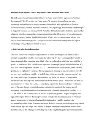
  • 5. for each training point of the form (x1, x2, x3, …, y). To make this process clearer, let us return to the example where we are predicting heights and let us apply least squares to a specific data set. Suppose that our training data consists of (weight, age, height) data for 7 people (which, in practice, is a very small amount of data). For example, we might have: Person 1: (160 pounds, 19 years old, 66 inches) Person 2: (172 pounds, 26 years old, 69 inches) Person 3: (178 pounds, 23 years old, 72 inches) Person 4: (170 pounds, 70 years old, 69 inches) Person 5: (140 pounds, 15 years old, 68 inches) Person 6: (169 pounds, 60 years old, 67 inches) Person 7: (210 pounds, 41 years old, 73 inches) This training data can be visualized, as in the image below, by plotting each training point in a three dimensional space, where one axis corresponds to height, another to weight, and the third to age:
  • 6. As we have said, the least squares method attempts to minimize the sum of the squared error between the values of the dependent variables in our training set, and our model’s predictions for these values. Hence, in this case it is looking for the constants c0, c1 and c2 to minimize: Sum of Squared Errors = (66 – (c0 + c1*160 + c2*19))^2 + (69 – (c0 + c1*172 + c2*26))^2 + (72 – (c0 + c1*178 + c2*23))^2 + (69 – (c0 + c1*170 + c2*70))^2 + (68 – (c0 + c1*140 + c2*15))^2 + (67 – (c0 + c1*169 + c2*60))^2 + (73 – (c0 + c1*210 + c2*41))^2 The solution to this minimization problem happens to be given by c0 = 52.8233 (inches) c1 = 0.101546 (inches per pound) c2 = -0.0295932 (inches per year) Sum of Squared Errors = 14.1469 which means then that we can attempt to estimate a person’s height from their age and weight using the following formula: height = 52.8233 – 0.0295932 age + 0.101546 weight. In practice however, this formula will do quite a bad job of predicting heights, and in fact illustrates some of the problems with the way that least squares regression is often applied in practice (as will be discussed in detail later on in this essay). This solution for c0, c1, and c2 (which can be thought of as the plane 52.8233 – 0.0295932 x1 + 0.101546 x2) can be visualized as:
  • 7. That means that for a given weight and age we can attempt to estimate a person’s height by simply looking at the “height” of the plane for their weight and age. Why Is Least Squares So Popular? We’ve now seen that least squared regression provides us with a method for measuring “accuracy” (i.e. the sum of squared errors) and that is what makes it different from other forms of linear regression. However, least squares is such an extraordinarily popular technique that often when people use the phrase “linear regression” they are in fact referring to “least squares regression”. But why should people think that least squares regression is the “right” kind of linear regression? And more generally, why do people believe that linear regression (as opposed to non-linear regression) is the best choice of regression to begin with? Unfortunately, the popularity of least squares regression is, in large part, driven by a series of factors that have little to do with the question of what technique actually makes the most useful predictions in practice. Much of the use of least squares can be attributed to the following factors: (a) It was invented by Carl Friedrich Gauss (one of the world’s most famous mathematicians) in about 1795, and then rediscovered by Adrien-Marie Legendre (another famous mathematician) in 1805, making it one of the earliest general prediction methods known to humankind. (b) It is easy to implement on a computer using commonly available algorithms from linear algebra.
  • 8. (c) Its implementation on modern computers is efficient, so it can be very quickly applied even to problems with hundreds of features and tens of thousands of data points. (d) It is easier to analyze mathematically than many other regression techniques. (e) It is not too difficult for non-mathematicians to understand at a basic level. (f) It produces solutions that are easily interpretable (i.e. we can interpret the constants that least squares regression solves for). (g) It is the optimal technique in a certain sense in certain special cases. In particular, if the system being studied truly is linear with additive uncorrelated normally distributed noise (of mean zero and constant variance) then the constants solved for by least squares are in fact the most likely coefficients to have been used to generate the data. There is also the Gauss-Markov theorem which states that if the underlying system we are modeling is linear with additive noise, and the random variables representing the errors made by our ordinary least squares model are uncorrelated from each other, and if the distributions of these random variables all have the same variance and a mean of zero, then the least squares method is the best unbiased linear estimator of the model coefficients (though not necessarily the best biased estimator) in that the coefficients it leads to have the smallest variance. While some of these justifications for using least squares are compelling under certain circumstances, our ultimate goal should be to find the model that does the best job at making predictions given our problem’s formulation and constraints (such as limited training points, processing time, prediction time, and computer memory). Problems and Pitfalls of Applying Least Squares Regression Unfortunately, as has been mentioned above, the pitfalls of applying least squares are not sufficiently well understood by many of the people who attempt to apply it. What follows is a list of some of the biggest problems with using least squares regression in practice, along with some brief comments about how these problems may be mitigated or avoided: 1. Outliers
  • 9. Least squares regression can perform very badly when some points in the training data have excessively large or small values for the dependent variable compared to the rest of the training data. The reason for this is that since the least squares method is concerned with minimizing the sum of the squared error, any training point that has a dependent value that differs a lot from the rest of the data will have a disproportionately large effect on the resulting constants that are being solved for. To further illuminate this concept, lets go back again to our example of predicting height. Due to the squaring effect of least squares, a person in our training set whose height is mispredicted by four inches will contribute sixteen times more error to the summed of squared errors that is being minimized than someone whose height is mispredicted by one inch. That means that the more abnormal a training point’s dependent value is, the more it will alter the least squares solution. Hence a single very bad outlier can wreak havoc on prediction accuracy by dramatically shifting the solution. If the outlier is sufficiently bad, the value of all the points besides the outlier will be almost completely ignored merely so that the outlier’s value can be predicted accurately. In the images below you can see the effect of adding a single outlier (a 10 foot tall 40 year old who weights 200 pounds) to our old training set from earlier on. Here we see a plot of our old training data set (in purple) together with our new outlier point (in green): Below we have a plot of the old least squares solution (in blue) prior to adding the outlier point to our training set, and the new least squares solution (in green) which is attained after the outlier is added:
  • 10. As you can see in the image above, the outlier we added dramatically distorts the least squares solution and hence will lead to much less accurate predictions. The problem of outliers does not just haunt least squares regression, but also many other types of regression (both linear and non-linear) as well. One partial solution to this problem is to measure accuracy in a way that does not square errors. For example, the least absolute errors method (a.k.a. least absolute deviations, which can be implemented, for example, using linear programming or the iteratively weighted least squares technique) will emphasize outliers far less than least squares does, and therefore can lead to much more robust predictions when extreme outliers are present. An even more outlier robust linear regression technique is least median of squares, which is only concerned with the median error made on the training data, not each and every error. Unfortunately, this technique is generally less time efficient than least squares and even than least absolute deviations. Another solution to mitigate these problems is to preprocess the data with an outlier detection algorithm that attempts either to remove outliers altogether or de-emphasize them by giving them less weight than other points when constructing the linear regression model. Though sometimes very useful, these outlier detection algorithms unfortunately have the potential to bias the resulting model if they accidently remove or de-emphasize the wrong points. Regression
  • 11. methods that attempt to model data on a local level (like local linear regression) rather than on a global one (like ordinary least squares, where every point in the training data effects every point in the resulting shape of the solution curve) can often be more robust to outliers in the sense that the outliers will only distrupt the model in a small region rather than disrupting the entire model. It should be noted that bad outliers can sometimes lead to excessively large regression constants, and hence techniques like ridge regression and lasso regression (which dampen the size of these constants) may perform better than least squares when outliers are present. One thing to note about outliers is that although we have limited our discussion here to abnormal values in the dependent variable, unusual values in the features of a point can also cause severe problems for some regression methods, especially linear ones such as least squares. The trouble is that if a point lies very far from the other points in feature space, then a linear model (which by nature attributes a constant amount of change in the dependent variable for each movement of one unit in any direction) may need to be very flat (have constant coefficients close to zero) in order to avoid overshooting the far away point by an enormous amount. Hence, points that are outliers in the independent variables can have a dramatic effect on the final solution, at the expense of achieving a lot of accuracy for most of the other points. 2. Non-Linearities All linear regression methods (including, of course, least squares regression), suffer from the major drawback that in reality most systems are not linear. As we have discussed, linear models attempt to fit a line through one dimensional data sets, a plane through two dimensional data sets, and a generalization of a plane (i.e. a hyperplane) through higher dimensional data sets. In practice though, real world relationships tend to be more complicated than simple lines or planes, meaning that even with an infinite number of training points (and hence perfect information about what the optimal choice of plane is) linear methods will often fail to do a good job at making predictions. For example, trying to fit the curve y = 1-x^2 by training a linear regression model on x and y samples taken from this function will lead to disastrous results, as is shown in the image below. The line depicted is the least squares solution line, and the points are values of 1-x^2 for random choices of x taken from the interval [-1,1].
  • 12. Notice that the least squares solution line does a terrible job of modeling the training points. In this problem, when a very large numbers of training data points are given, a least squares regression model (and almost any other linear model as well) will end up predicting that y is always approximately zero. Sometimes 1-x^2 is above zero, and sometimes it is below zero, but on average there is no tendency for 1-x^2 to increase or decrease as x increases, which is what linear models capture. Examples like this one should remind us of the saying, “attempting to divide the world into linear and non-linear problems is like trying to dividing organisms into chickens and non-chickens”. When you have a strong understanding of the system you are attempting to study, occasionally the problem of non-linearity can be circumvented by first transforming your data in such away that it becomes linear (for example, by applying logarithms or some other function to the appropriate independent or dependent variables). In practice though, knowledge of what transformations to apply in order to make a system linear is typically not available. Furthermore, while transformations of independent variables is usually okay, transformations of the dependent variable will cause distortions in the manner that the regression model measures errors, hence producing what are often undesirable results. Another possibility, if you precisely know the (non-linear) model that describes your data but aren’t sure about the values of some parameters of this model, is to attempt to directly solve for the optimal choice of these parameters that minimizes some notion of prediction error (or,
  • 13. equivalently, maximizes some measure of accuracy). This is sometimes known as parametric modeling, as opposed to the non-parametric modeling which will be discussed below. To give an example, if we somehow knew that y = 2^(c0*x) + c1 x + c2 log(x) was a good model for our system, then we could try to calculate a good choice for the constants c0, c1 and c2 using our training data (essentially by finding the constants for which the model produces the least error on the training data points). There are a variety of ways to do this, for example using a maximal likelihood method or using the stochastic gradient descent method. Much of the time though, you won’t have a good sense of what form a model describing the data might take, so this technique will not be applicable. Another method for avoiding the linearity problem is to apply a non-parametric regression method such as local linear regression (a.k.a. local least squares or locally weighted scatterplot smoothing, which can work very well when you have lots of training data and only relatively small amounts of noise in your data) or a kernel regression technique (like the Nadaraya-Watson method). Both of these approaches can model very complicated systems, requiring only that some weak assumptions are met (such as that the system under consideration can be accurately modeled by a smooth function). These non-parametric algorithms usually involve setting a model parameter (such as a smoothing constant for local linear regression or a bandwidth constant for kernel regression) which can be estimated using a technique like cross validation. A troublesome aspect of these approaches is that they require being able to quickly identify all of the training data points that are “close to” any given data point (with respect to some notion of distance between points), which becomes very time consuming in high dimensional feature spaces (i.e. when there are a large number of independent variables). Even worse, when we have many independent variables in our model, the performance of these methods can rapidly erode. Yet another possible solution to the problem of non-linearities is to apply transformations to the independent variables of the data (prior to fitting a linear model) that map these variables into a higher dimension space. If the transformation is chosen properly, then even if the original data is not well modeled by a linear function, the transformed data will be. A very simple and naive use of this procedure applied to the height prediction problem (discussed previously) would be to take our two independent variables (weight and age) and transform them into a set of five
  • 14. independent variables (weight, age, weight*age, weight^2 and age^2), which brings us from a two dimensional feature space to a five dimensional one. Our model would then take the form: height = c0 + c1*weight + c2*age + c3*weight*age + c4*weight^2 + c5*age^2 This new model is linear in the new (transformed) feature space (weight, age, weight*age, weight^2 and age^2), but is non-linear in the original feature space (weight, age). The procedure used in this example is very ad hoc however and does not represent how one should generally select these feature transformations in practice (unless a priori knowledge tells us that this transformed set of features would be an adequate choice). To automate such a procedure, the Kernel Principle Component Analysis technique and other so called Nonlinear Dimensionality Reduction techniques can automatically transform the input data (non-linearly) into a new feature space that is chosen to capture important characteristics of the data. When a linear model is applied to the new independent variables produced by these methods, it leads to a non-linear model in the space of the original independent variables. A related (and often very, very good) solution to the non-linearity problem is to directly apply a so-called “kernel method” like support vector regression or kernelized ridge regression (a.k.a. kernelized Tikhonov regularization) with an appropriate choice of a non-linear kernel function. These methods automatically apply linear regression in a non-linearly transformed version of your feature space (with the actual transformation used determined by the choice of kernel function) which produces non-linear models in the original feature space. Certain choices of kernel function, like the Gaussian kernel (sometimes called a radial basis function kernel or RBF kernel), will lead to models that are consistent, meaning that they can fit virtually any system to arbitrarily good accuracy, so long as a sufficiently large amount of training data points are available. All regular linear regression algorithms conspicuously lack this very desirable property. It should be noted that when the number of input variables is very large, the restriction of using a linear model may not be such a bad one (because the set of planes in a very large dimensional space may actually be quite a flexible model). Furthermore, when we are dealing with very noisy data sets and a small numbers of training points, sometimes a non-linear model is too much to
  • 15. ask for in a sense because we don’t have enough data to justify a model of large complexity (and if only very simple models are possible to use, a linear model is often a reasonable choice). That being said (as shall be discussed below) least squares regression generally performs very badly when there are too few training points compared to the number of independent variables, so even scenarios with small amounts of training data often do not justify the use of least squares regression. These scenarios may, however, justify other forms of linear regression. An important idea to be aware of is that it is typically better to apply a method that will automatically determine how much complexity can be afforded when fitting a set of training data than to apply an overly simplistic linear model that always uses the same level of complexity (which may, in some cases be too much, and overfit the data, and in other cases be too little, and underfit it). When the support vector regression technique and ridge regression technique use linear kernel functions (and hence are performing a type of linear regression) they generally avoid overfitting by automatically tuning their own levels of complexity, but even so cannot generally avoid underfitting (since linear models just aren’t complex enough to model some systems accurately when given a fixed set of features). The kernelized (i.e. non-linear) versions of these techniques, however, can avoid both overfitting and underfitting since they are not restricted to a simplistic linear model. 3. Too Many Variables While intuitively it seems as though the more information we have about a system the easier it is to make predictions about it, with many (if not most) commonly used algorithms the opposite can occasionally turn out to be the case. While it never hurts to have a large amount of training data (except insofar as it will generally slow down the training process), having too many features (i.e. independent variables) can cause serious difficulties. Least squares regression is particularly prone to this problem, for as soon as the number of features used exceeds the number of training data points, the least squares solution will not be unique, and hence the least squares algorithm will fail. In practice, as we add a large number of independent variables to our least squares model, the performance of the method will typically erode before this critical point (where the number of features begins to exceed the number of training points) is reached. This implies that rather than just throwing every independent variable we have access to into our regression model, it can be beneficial to only include those features that are likely to be good
  • 16. predictors of our output variable (especially when the number of training points available isn’t much bigger than the number of possible features). What’s more, we should avoid including redundant information in our features because they are unlikely to help, and (since they increase the total number of features) may impair the regression algorithm’s ability to make accurate predictions. Keep in mind that when a large number of features is used, it may take a lot of training points to accurately distinguish between those features that are correlated with the output variable just by chance, and those which meaningfully relate to it. Some regression methods (like least squares) are much more prone to this problem than others. As the number of independent variables in a regression model increases, its R^2 (which measures what fraction of the variability (variance) in the training data that the prediction method is able to account for) will always go up. This increase in R^2 may lead some inexperienced practitioners to think that the model has gotten better. When applying least squares regression, however, it is not the R^2 on the training data that is significant, but rather the R^2 that the model will achieve on the data that we are interested in making prediction for (i.e. we care about error on the test set, not the training set). When too many variables are used with the least squares method the model begins finding ways to fit itself to not only the underlying structure of the training set, but to the noise in the training set as well, which is one way to explain why too many features leads to bad prediction results. One way to help solve the problem of too many independent variables is to scrutinize all of the possible independent variables, and discard all but a few (keeping a subset of those that are very useful in predicting the dependent variable, but aren’t too similar to each other). For least squares regression, the number of independent variables chosen should be much smaller than the size of the training set. This approach can be carried out systematically by applying a feature selection or dimensionality reduction algorithm (such as subset selection, principal component analysis, kernel principal component analysis, or independent component analysis) to preprocess the data and automatically boil down a large number of input variables into a much smaller number. Some of these methods automatically remove many of the features, whereas others combine features together into a smaller number of new features. These algorithms can be very useful in practice, but occasionally will eliminate or reduce the importance of features that are very important, leading to bad predictions. It is crtitical that, before certain of these feature selection
  • 17. methods are applied, the independent variables are normalized so that they have comparable units (which is often done by setting the mean of each feature to zero, and the standard deviation of each feature to one, by use of subtraction and then division). Another approach to solving the problem of having a large number of possible variables is to use lasso linear regression which does a good job of automatically eliminating the effect of some independent variables. Other regression techniques that can perform very well when there are very large numbers of features (including cases where the number of independent variables exceeds the number of training points) are support vector regression, ridge regression, and partial least squares regression. 4. Dependence Among Variables The least squares method can sometimes lead to poor predictions when a subset of the independent variables fed to it are significantly correlated to each other. The problem in these circumstances is that there are a variety of different solutions to the regression problem that the model considers to be almost equally good (as far as the training data is concerned), but unfortunately many of these “nearly equal” solutions will lead to very bad predictions (i.e. poor performance on the testing set). To illustrate this point, lets take the extreme example where we use the same independent variable twice with different names (and hence have two input variables that are perfectly correlated to each other). If these perfectly correlated independent variables are called w1 and w2, then we note that our least squares regression algorithm doesn’t distinguish between the two solutions y = .5*w1 + .5*w2 and y = 1000*w1 – 999*w2 since .5*w1 + .5*w2 = .5*w1 + .5*w1 = w1
  • 18. and 1000*w1 – 999*w2 = 1000*w1 – 999*w1 = w1. In both cases the models tell us that y tends to go up on average about one unit when w1 goes up one unit (since we can simply think of w2 as being replaced with w1 in these equations, as was done above). Intuitively though, the second model is likely much worse than the first, because if w2 ever begins to deviate even slightly from w1 the predictions of the second model will change dramatically. For example, if for a single prediction point w2 were equal to .95 w1 rather than the precisely one w1 that we expected, then we would find that the first model would give the prediction y = .5*w1 + .5*w2 = .5*w1 + .5*0.95*w1 = 0.975 w1 which is very close to the prediction of simply one w1 that we get without this change in w2. On the other hand, in these circumstances the second model would give the prediction y = 1000*w1 – 999*w2 = 1000*w1 – 999*0.95*w1 = 50.95 w1 which isn’t even close to our old prediction of just one w1. Hence we see that dependencies in our independent variables can lead to very large constant coefficients in least squares regression, which produce predictions that swing wildly and insanely if the relationships that held in the training set (perhaps, only by chance) do not hold precisely for the points that we are attempting to make predictions on. A common solution to this problem is to apply ridge regression or lasso regression rather than least squares regression. Both of these methods have the helpful advantage that they try to avoid producing models that have large coefficients, and hence often perform much better when strong dependencies are present. It should be noted that when the number of training points is sufficiently large (for the given number of features in the problem and the distribution of noise) correlations among the features may not be at all problematic for the least squares method. On the other hand though, when the number of training points is insufficient, strong correlations can lead to very bad results.
  • 19. 5. Wrong Choice of Error Function As we have said before, least squares regression attempts to minimize the sum of the squared differences between the values predicted by the model and the values actually observed in the training data. More formally, least squares regression is trying to find the constant coefficients c1, c2, c3, …, cn to minimize the quantity (y – (c1 x1 + c2 x2+ c3 x3 + … + cn xn))^2 when it is summed over each of the different training points (i.e. different know values for y, x1, x2, x3, …, xn). But why is it the sum of the squared errors that we are interested in? Is mispredicting one person’s height by two inches really as equally “bad” as mispredicting four people’s height by 1 inch each, as least squares regression implicitly assumes? Should mispredicting one person’s height by 4 inches really be precisely sixteen times “worse” than mispredicting one person’s height by 1 inch? This (not necessarily desirable) result is a consequence of the method for measuring error that least squares employs. In general we would rather have a small sum of squared errors rather than a large one (all else being equal), but that does not mean that the sum of squared errors is the best measure of error for us to try and minimize. The simple conclusion is that the way that least squares regression measures error is often not justified. Lets use a simplistic and artificial example to illustrate this point. Suppose that we are in the insurance business and have to predict when it is that people will die so that we can appropriately value their insurance policies. Furthermore, suppose that when we incorrectly identify the year when a person will die, our company will be exposed to losing an amount of money that is proportional to the absolute value of the error in our prediction. In other words, if we predict that someone will die in 1993, but they actually die in 1994, we will lose half as much money as if they died in 1995, since in the latter case our estimate was off by twice as many years as in the former case. What’s more, in this scenario, missing someone’s year of death by two years is precisely as bad to us as mispredicting two people’s years of death by one year each (since the same number of dollars will be lost by us in both cases). If we are concerned with losing as little money as possible, then it is is clear that the right notion of error to minimize in our model is the
  • 20. sum of the absolute value of the errors in our predictions (since this quantity will be proportional to the total money lost), not the sum of the squared errors in predictions that least squares uses. In some many cases we won’t know exactly what measure of error is best to minimize, but we may be able to determine that some choices are better than others. The point is, if you are interested in doing a good job to solve the problem that you have at hand, you shouldn’t just blindly apply least squares, but rather should see if you can find a better way of measuring error (than the sum of squared errors) that is more appropriate to your problem. Sum of squared error minimization is very popular because the equations involved tend to work out nice mathematically (often as matrix equations) leading to algorithms that are easy to analyze and implement on computers. But frequently this does not provide the best way of measuring errors for a given problem. It should be noted that there are certain special cases when minimizing the sum of squared errors is justified due to theoretical considerations. One such justification comes from the relationship between the sum of squares and the arithmetic mean (usually just called “the mean”). Suppose that we have samples from a function that we are attempting to fit, where noise has been added to the values of the dependent variable, and the distribution of noise added at each point may depend on the location of that point in feature space. In that case, if we have a (parametric) model that we know encompasses the true function from which the samples were drawn, then solving for the model coefficients by minimizing the sum of squared errors will lead to an estimate of the true function’s mean value at each point. On the other hand, if we instead minimize the sum of the absolute value of the errors, this will produce estimates of the median of the true function at each point. Hence, in cases such as this one, our choice of error function will ultimately determine the quantity we are estimating (function(x) + mean(noise(x)), function(x) + median(noise(x)), or what have you). Since the mean has some desirable properties and, in particular, since the noise term is sometimes known to have a mean of zero, exceptional situations like this one can occasionally justify the minimization of the sum of squared errors rather than of other error functions. 6. Unequal Training Point Variances (Heteroskedasticity)
  • 21. Interestingly enough, even if the underlying system that we are attempting to model truly is linear, and even if (for the task at hand) the best way of measuring error truly is the sum of squared errors, and even if we have plenty of training data compared to the number of independent variables in our model, and even if our training data does not have significant outliers or dependence between independent variables, it is STILL not necessarily the case that least squares (in its usual form) is the optimal model to use. The difficulty is that the level of noise in our data may be dependent on what region of our feature space we are in. For example, going back to our height prediction scenario, there may be more variation in the heights of people who are ten years old than in those who are fifty years old, or there more be more variation in the heights of people who weight 100 pounds than in those who weight 200 pounds. The upshot of this is that some points in our training data are more likely to be effected by noise than some other such points, which means that some points in our training set are more reliable than others. We don’t want to ignore the less reliable points completely (since that would be wasting valuable information) but they should count less in our computation of the optimal constants c0, c1, c2, …, cn than points that come from regions of space with less noise. To do this one can use the technique known as weighted least squares which puts more “weight” on more reliable points. In practice though, since the amount of noise at each point in feature space is typically not known, approximate methods (such as feasible generalized least squares) which attempt to estimate the optimal weight for each training point are used. 7. Wrong Choice of Features The problem of selecting the wrong independent variables (i.e. features) for a prediction problem is one that plagues all regression methods, not just least squares regression. To illustrate this problem in its simplest form, suppose that our goal is to predict people’s IQ scores, and the features that we are using to make our predictions are the average number of hours that each person sleeps at night and the number of children that each person has. Clearly, using these features the prediction problem is essentially impossible because their is so little relationship (if any at all) between the independent variables and the dependent variable. No model or learning algorithm no matter how good is going to rectify this situation. What’s worse, if we have very limited amounts of training data to build our model from, then our regression algorithm may even discover spurious relationships between the independent variables and dependent variable
  • 22. that only happen to be there due to chance (i.e. random fluctuation). Even if many of our features are in fact good ones, the genuine relations between the independent variables the dependent variable may well be overwhelmed by the effect of many poorly selected features that add noise to the learning process. When carrying out any form of regression, it is extremely important to carefully select the features that will be used by the regression algorithm, including those features that are likely to have a strong effect on the dependent variable, and excluding those that are unlikely to have much effect. 8. Noise in the Independent Variables While least squares regression is designed to handle noise in the dependent variable, the same is not the case with noise (errors) in the independent variables. Noise in the features can arise for a variety of reasons depending on the context, including measurement error, transcription error (if data was entered by hand or scanned into a computer), rounding error, or inherent uncertainty in the system being studied. Models that specifically attempt to handle cases such as these are sometimes known as errors in variables models. When a substantial amount of noise in the independent variables is present, the total least squares technique (which measures error using the distance between training points and the prediction plane, rather than the difference between the training point dependent variables and the predicted values for these variables) may be more appropriate than ordinary least squares. Another option is to employ least products regression. Conclusion Although least squares regression is undoubtedly a useful and important technique, it has many defects, and is often not the best method to apply in real world situations. A great deal of subtlety is involved in finding the best solution to a given prediction problem, and it is important to be aware of all the things that can go wrong.