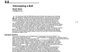
SlideShare uma empresa Scribd logo
1 de 8
9.8
Intercepting a Ball
Noah Stein
noah@acm.org
J ohn Stockton holds the NBA all-time record for the most steals by an individual
throughout his career-more than 2,800 (as of2001). He has more than luck. He
has skill. However, his skill is not merely confined to the mechanical act of stealing
the ball. As imponant as the motion itself, he has skill in determining when he can
steal the ball. Without the when, he would never have the chance to use the how.
In sports games, many situations arise that require determining whether a pl ay er
can intercept the ball: a second baseman wants to catch a line drive, a hockey wing
tries to steal a pass, a soccer goalie needs to block a shot, or a basketball center wishes
to rebound the ball. In these cases, the AI needs to decide if the action can be success
fully executed, or whether an alternative course of action should be taken.
The algorithm described herein is also applicable outside the genre of sports
games: the Shao-Lin master might need to decide whether to grab an arrow flying at
him or just move his leg out of the way. Can the Patriot missile intercept and destroy
the Scud? A secret service agent needs to know if he can dive in front of the President
and take the bullet in time.
The Basic Problem
The previous examples can be distilled down to essentially the same problem: one
object is at a certain position (P b ) and traveling in a straight line at a constant velocity
(Vb); another object at a different position (P p ) wants to intercept the first, but it
might not move faster than a specific speed (s). From this information, the model
solves for the second object's velocity to intercept (i,;,). Some might object to the sim
plicity of the model; however, every model must make simplifications, and those
made for this problem render a functional solution. Please note that in the discussion
that follows, the ball is the object that is traveling along a path that is to be inter
cepted, and the player is the object that wants to intercept the ball.
The first simplification is that the ball's velocity is constant and its trajectory is
therefore a straight line. A basketball coming off the rim follows a parabolic trajec
tory-not even remotely close to a straight line. How can a straight line model the
motion effectively? This model can be broken down into two independent submod
els: the altitude of the ball, and the motion in the ground plane. Because the two axes
496 Section 9 Racing and Sports Al
in the ground plane are orthogonal to the altitude axis, their motions can be consid
ered in isolation [Resnick91]. The bulk of this article explains the computation of the
ground plane interception. The end of the article addresses adding altitude consider
ations to the model.
The second simplification is that the intercepting object has no turning radius,
infinite acceleration, and can travel indefinitely at its maximum velocity. This is defi
nitely the more difficult of the two aspects to explain, because it will introduce the
most error. First, error isn't necessarily a bad thing: a real person will have difficulty
judging certain situations. Second, there are other methods that can be used to com
pensate for heading changes, some of which appear later. In addition, the interplay
between changes of direction and acceleration is so complex that a simplification to
some degree must occur.
Given this information, the model has four independent variables: the position of
the ball, the velocity of the ball, the position of the interceptor, and the maximum
speed the interceptor can travel. A graphical representation of the problem is shown
in Figure 9 .8.1. Please note that in all figures, dots represent the objects, solid lines
represent velocities, and dashed lines represent changes in position.
O ······
➔
? A ?
't: : -:1
••
t=0
0------ ➔
? A ?
�. : ..�
·-
....•....
··
t = 1
FIGURE 9.8.1 The intercept ball problem.
O ······➔
�
? ?
�--. • .,. -:1
·--.........
·····
Deriving the Solution
Examining Figure 9.8.1, the problem might appear to be the point on line closest to
point algorithm from Graphics Gems [Glassner90]. The check determines the closest
point on the trajectory line. It appears to be a good choice. In some cases, the optimal
choice is close to this point; however, Figure 9.8.2 clearly illustrates a case in which
the point-line test clearly and convincingly fails to deliver the correct result.
What is the proper mathematical model? For an interception to occur, the posi
tion of both the ball and the player must be the same at some time t. Thus, if V P was
known a priori, the intercept statement would appear as such:
P b + V b t == P p + vl (9.8.1)
9,8 Intercepting a Ball 497
O· ·····➔ O ······
➔
FIGURE 9.8.2 Failure to intercept the ball given the simple solution of choosing the closest
point on the ball's trajectory.
Unfortunately, V P is the variable to be solved. The solution requires that the
problem be viewed from a different vantage. If the positions of the player and ball are
the same, the distance must be 0. The distance between the player's initial position
and the ball at time r.
(9.8.2)
In Equation 9.8.2, the vector can be considered to be composed of two elements:
the initial position of the ball relative to the player (the part in the parentheses), and
the motion of the ball due to its velocity vector. If the player can move a distance
equivalent to how distant the ball is, the player can intercept the ball at time t:
(9.8.3)
Since the initial positions never change, to simplify further discussion, the substi
tution P =P b - P; will be made from this point forth. In addition, subscripts will be
dropped since there will be no ambiguity in the text. Solving for t results in the
time(s) at which the player can successfully intercept the ball:
IP+ Vt != st
.J(P +Vt}• (P + Vt} = st
(P +Vt}• (P +Vt)= (st)
2
P • P + 2P • Vt+ V • Vt 2
= s2
t 2
(V • V - s
2
)t 2 + ( 2P • V )t + ( P • P) = 0 (9.8.4)
Now the equation is a second-order polynomial oft. Plug the polynomial scalars
into the quadratic equation.
498 Section 9 Racing and Sports Al
-----
Analysis of the Quadratic
- b ± ✓
b 2 - 4ac
2a
(9.8 .5)
The quadratic equation has three different categories of solutions: no real roots,
one real root, and two real roots. The category of solution is determined by the
expression in the radical: b2 -4ac. If it is negative, the solution has no real roots. If it
is zero, the radical after the "±" is zero and results in a single real root. If greater than
zero, the solution has two real roots. But what does this mean? First, let's transform
the expression in the radical into a more informative form for subsequent analysis:
b 2 - 4 ac = (2P • v) 2
- 4 (v • v - s2
)(r • r)
= 4(P • V
r -4(V • V - s2
)( P • P)
= (P • vr -(v • V - s2
)(r • P )
= (r • v) 2
+ (s2 - v • v )(r • r )
No Real Roots
(9. 8 .6 )
If the radicand (the quantity within the radical ) is negative, then there are no real
roots, and the ball cannot be intercepted. In this case, the quantity (s 2 - V • V) must
be negative, so s</V/. Only when the ball travels at a speed greater than the maximum
speed of the player will chis case occur. This agrees with our intuition that the player
has co be able to move faster than the ball if he ever hopes co intercept its path.
One Real Root
This case represents a border case between whether or not the player can intercept
the ball. The interception is so difficult that there is only one point in time chat the
ball can be intercepted. For the quadratic equation to result in a single root, the radi
cand must be zero. Examining Equation 9.8.6, if the initial positions coincide, the
radical is zero, because both addends have multiplicands that have doc products
involving P, resulting in zeros. Equation 9.8.5 reduces to:
- b - (P • v )
2 a 2(v • v - s2
)
To fully understand the single real root case, Equation 9.8.7 must be considered
in light of the face that the radicand is zero. From Equation 9.8.6:
9.8 Intercepting a Ball 499
(P • v)
2
+ (s2
- V • v )(P • P) = 0
( P • V )
2
= - ( s2
- V • V )(P • P) (9.8.8)
Since the left side must be positive (due to the square), the right side must be neg
ative; therefore, the interceptor is faster than the ball. Examining Equation 9.8.7 with
that knowledge, the divisor must be negative in this case. Our analysis of the single
real root has two subcases:
• (P•V)<O: The ball's velocity is roughly toward the interceptor, thus it can be inter
cepted at some point in the future. The numerator becomes negative (because of
the negative sign), so the equation has a positive result. Since the ball moves faster
than the interceptor, it can only be intercepted at one point in time. After that time,
it will be traveling too quickly to be reached again. This is akin to the second base
man grabbing a line drive: if it shoots by in arm's reach, he can grab it in his imme
diate vicinity, but he'll never have a chance to catch it in the outfield.
• (P•V)>O: The ball's velocity is not toward the interceptor in any conceivable way.
So, how is it that there is a root? With the dividend negative, the result is nega
tive. Thus, the interception occurred in the past. Since time only moves forward,
this result indicates that the result should be discarded.
Two Real Roots
The final case is the mo st interesting. This case does not require the speed of the
pl ay er to be greater. Although the ball can move significantly faster than the player, if
the player is sufficiently far away from the ball's initial position, but near the line in
positive t, the ball can be intercepted.
The two real roots represent the boundaries of a window of opportunity; how
ever, their interpretation falls into three categories, depending on the sign of the roots:
two positive roots, two negative roots, and one positive and one negative root.
• Two p ositive roots: The roots define a window of opportunity in which the ball
can be successfully intercepted. Any time between the two roots is a valid time at
which the ball can be intercepted. In this scenario, the ball is moving faster than
the pl ay er, but the player is, relative to the ratio of speed and distance, close to the
line of motion and thus can make it there in time.
• Two negative roots: The roots also define a window of opportunity between the
two values in which the ball can be intercepted. It also has the property of the ball
moving faster than the pl ay er; however, the ball is moving entirely away from the
player. Thus, the window is entirely in negative time, so this result is to be dis
carded as an impossible interception.
• One p ositive and one negative root: The solution has two open-ended windows
of opportunity: time less than or equal to the negative root, and time greater than
500 Section 9 Racing and Sports Al
is to be discarded. In this scenario, the player is moving faster than the ball, and
thus can reach at any time after a certain minimum needed to catch it.
Choosing the Time to Meet
Once the root or roots are known, a valid time can be plugged back into the first
equation in Equation 9.8.4, resulting in the point at which the target can be inter
cepted. Of the three root categories, only the two real roots case affords the AI discre
tion in choosing at which time the player would like to intercept the ball. In the no
real roots case, the ball cannot be intercepted, and with a single real root, there is a
unique time at which the interception could occur.
The two real roots case, in contrast, defines an interval of time in which the ball
can be intercepted. What is the best time to choose? The obvious answer is a root
itsel£ Although the only answer for the single real root case, it is probably not the best
choice in the two-root case. To illustrate, imagine one person passing the ball to
another. T he passer throws the ball just beyond the receiver's reach. The receiver
could take two leisurely steps perpendicular to the path of the ball and grab it. If a
root is chosen, he will run as fast as he can to catch the ball, running mostly in a direc
tion parallel to the motion of the ball.
Thus, for a more realistic decision, a time somewhere in the middle of interval
should be chosen. T ry to find the "lazy" point-the solution requiring the least
amount of effort to still create an interception outcome. How can the lazy point be
determined? We know two aspects of the solution: 1) the speed of interception should
be as small as possible, yet still allow an interception to occur, and 2) at the minimum
allowed interception speed, there is only one possible point in time to intercept, so
there must be only one real root. For one real root, the expression under the radical
must be zero. Solve for s:
(P • V
r+ ( s
2
- V • V ) (P • P) = O
(P • v f + s
2
(P • P)- (v • v) (P • P) = 0
2 _ ( V • V )( P • P) - ( P • V
r
s
s =
(P • P)
(v • v)( P • P )- ( P • v f
(P • P)
(9.8.9)
9.8 Intercepting a Ball 501
The solution for s in Equation 9.8.9 must then be plugged back into the qua
dratic equation to give the resulting time of interception that can then be used to
compute the location of intersection.
Related Problems
Now that the essential model has been fully constructed and anal yz ed, let's briefly
summarize two variants:
1. The pl ay er has long arms that the model should consider. T he arms can be
modeled effectively as a nonzero initial position. If the player's arms are l
long, Equation 9.8.3 becomes:
l(Pb - P;) + V b t l = l + s;t (9.8.10)
The new solutions can be derived as above from this new equation.
2. Another consideration that might require modeling could be a del ay ed reac
tion by the player. Some developers' preference is to wait until such time as
the player can move on the ball to make the decision; however, your needs
might require a predetermination. As such, if the player has a delay of d
duration, Equation 9.8.3 becomes:
(9.8.11)
These two variants can be used together in a single statement by merely
replacing the t factor in Equation 9.8.10 with the (t-d} factor seen in Equa
tion 9.8.11.
Rebounding the Ball
In rebounding, the ball's altitude affects a player's ability to intercept a ball. As indi
cated at the beginning of the article, the model thus far only handles the relationship
between the ball and player in the ground plane. In rebounding and similar situa
tions, a second time window is computed. In general, the intersection of two parabo
las has four solutions; however, the alignment of the parabolas results in a single
i ntersection, with the exception of the case where the ball and player coincide. The
formulation of the equation is reminiscent of the planar check-if the altitude of
the player is greater than the ball, he can intercept it.
P + s t - 1/ gt 2
> p + s t - ½'gt 2
p p / 2 h b
2
(9.8.12)
502 Section 9 Racing and Sports Al
At time t greater than the right-hand side, the ball can be caught. In many situa
tions, P p must factor in the player's height and reach for acceptable results.
Once the altitude window has been determined, use the time value to trim down
the range returned by the plane check. Another modeling note: the interaction of ball
and backboard results in many motion discontinuities. The proper method of han
dling this is to perform one check for each region of continuous time.
Conclusion
This article presents a simple and concise method to determine if one object can be
intercepted by another. The check consists of little more than three dot products to
determine the coefficients of a quadratic equation. The value of the expression under
the radical in the quadratic equation discriminates between the three major cases:
interception is impossible, a single point in time to intercept, and a window of oppor
tunity for interception. If a window of opportunity is found, further analysis deter
mines the best choice in the window.
The algorithm operates on a much-simplified view of the game model. The sim
plified model increases the error of the check; however, the error can be reduced effec
tively by dividing up the problem space and running each parameterization through
the algorithm. The method's efficiency confers the advantage that it can be run
frequently.
References
[Anton00] Anton, Howard, Elementary Linear Algebra, 8 th
Ed., John Wiley & Sons,
2000.
[Glassner90] Glassner, Andrew, "Useful 2D Geometry," Graphics Gems, Academic
Press, 1990.
[Resnick91] Resnick, Robert, and Halliday, David, Physics, 4 th
Ed., Vol 1, John Wiley
& Sons, 1991.
[Spiegel97] Spiegel, Murray R., and Rabin, Schaum's Outline of College Algebra, 2 nd
Ed., McGraw-Hill Professional Publishing, 1997.

Mais conteúdo relacionado

Semelhante a Intercepting a Ball Algorithm

Ch 3 Two Dimensional Kinematics
Ch 3 Two Dimensional KinematicsCh 3 Two Dimensional Kinematics
Ch 3 Two Dimensional KinematicsScott Thomas
 
COORDINATE GEOMETRY (7.4 Equations of Loci).pptx
COORDINATE GEOMETRY (7.4 Equations of Loci).pptxCOORDINATE GEOMETRY (7.4 Equations of Loci).pptx
COORDINATE GEOMETRY (7.4 Equations of Loci).pptxMuslimah1983
 
College Physics 1st Edition Etkina Solutions Manual
College Physics 1st Edition Etkina Solutions ManualCollege Physics 1st Edition Etkina Solutions Manual
College Physics 1st Edition Etkina Solutions ManualHowardRichsa
 
Point Placement Algorithms: An Experimental Study
Point Placement Algorithms: An Experimental StudyPoint Placement Algorithms: An Experimental Study
Point Placement Algorithms: An Experimental StudyCSCJournals
 
Jee advanced-2020-paper-1-solution
Jee advanced-2020-paper-1-solutionJee advanced-2020-paper-1-solution
Jee advanced-2020-paper-1-solutionAnkitBiswas17
 
Report Proj Hrishi Anirudh
Report Proj Hrishi AnirudhReport Proj Hrishi Anirudh
Report Proj Hrishi Anirudhanirudh.s
 
Calculating the Angle between Projections of Vectors via Geometric (Clifford)...
Calculating the Angle between Projections of Vectors via Geometric (Clifford)...Calculating the Angle between Projections of Vectors via Geometric (Clifford)...
Calculating the Angle between Projections of Vectors via Geometric (Clifford)...James Smith
 

Semelhante a Intercepting a Ball Algorithm (14)

Signals and Systems Assignment Help
Signals and Systems Assignment HelpSignals and Systems Assignment Help
Signals and Systems Assignment Help
 
Ch 3 Two Dimensional Kinematics
Ch 3 Two Dimensional KinematicsCh 3 Two Dimensional Kinematics
Ch 3 Two Dimensional Kinematics
 
Ch02 ssm
Ch02 ssmCh02 ssm
Ch02 ssm
 
Ch09 ssm
Ch09 ssmCh09 ssm
Ch09 ssm
 
Unit 6.4
Unit 6.4Unit 6.4
Unit 6.4
 
COORDINATE GEOMETRY (7.4 Equations of Loci).pptx
COORDINATE GEOMETRY (7.4 Equations of Loci).pptxCOORDINATE GEOMETRY (7.4 Equations of Loci).pptx
COORDINATE GEOMETRY (7.4 Equations of Loci).pptx
 
College Physics 1st Edition Etkina Solutions Manual
College Physics 1st Edition Etkina Solutions ManualCollege Physics 1st Edition Etkina Solutions Manual
College Physics 1st Edition Etkina Solutions Manual
 
Point Placement Algorithms: An Experimental Study
Point Placement Algorithms: An Experimental StudyPoint Placement Algorithms: An Experimental Study
Point Placement Algorithms: An Experimental Study
 
Control chap7
Control chap7Control chap7
Control chap7
 
AP Physics
AP PhysicsAP Physics
AP Physics
 
Jee advanced-2020-paper-1-solution
Jee advanced-2020-paper-1-solutionJee advanced-2020-paper-1-solution
Jee advanced-2020-paper-1-solution
 
Unit 6.3
Unit 6.3Unit 6.3
Unit 6.3
 
Report Proj Hrishi Anirudh
Report Proj Hrishi AnirudhReport Proj Hrishi Anirudh
Report Proj Hrishi Anirudh
 
Calculating the Angle between Projections of Vectors via Geometric (Clifford)...
Calculating the Angle between Projections of Vectors via Geometric (Clifford)...Calculating the Angle between Projections of Vectors via Geometric (Clifford)...
Calculating the Angle between Projections of Vectors via Geometric (Clifford)...
 

Último

GenAI talk for Young at Wageningen University & Research (WUR) March 2024
GenAI talk for Young at Wageningen University & Research (WUR) March 2024GenAI talk for Young at Wageningen University & Research (WUR) March 2024
GenAI talk for Young at Wageningen University & Research (WUR) March 2024Jene van der Heide
 
CHROMATOGRAPHY PALLAVI RAWAT.pptx
CHROMATOGRAPHY  PALLAVI RAWAT.pptxCHROMATOGRAPHY  PALLAVI RAWAT.pptx
CHROMATOGRAPHY PALLAVI RAWAT.pptxpallavirawat456
 
Citronella presentation SlideShare mani upadhyay
Citronella presentation SlideShare mani upadhyayCitronella presentation SlideShare mani upadhyay
Citronella presentation SlideShare mani upadhyayupadhyaymani499
 
User Guide: Orion™ Weather Station (Columbia Weather Systems)
User Guide: Orion™ Weather Station (Columbia Weather Systems)User Guide: Orion™ Weather Station (Columbia Weather Systems)
User Guide: Orion™ Weather Station (Columbia Weather Systems)Columbia Weather Systems
 
Pests of soyabean_Binomics_IdentificationDr.UPR.pdf
Pests of soyabean_Binomics_IdentificationDr.UPR.pdfPests of soyabean_Binomics_IdentificationDr.UPR.pdf
Pests of soyabean_Binomics_IdentificationDr.UPR.pdfPirithiRaju
 
Servosystem Theory / Cybernetic Theory by Petrovic
Servosystem Theory / Cybernetic Theory by PetrovicServosystem Theory / Cybernetic Theory by Petrovic
Servosystem Theory / Cybernetic Theory by PetrovicAditi Jain
 
Radiation physics in Dental Radiology...
Radiation physics in Dental Radiology...Radiation physics in Dental Radiology...
Radiation physics in Dental Radiology...navyadasi1992
 
《Queensland毕业文凭-昆士兰大学毕业证成绩单》
《Queensland毕业文凭-昆士兰大学毕业证成绩单》《Queensland毕业文凭-昆士兰大学毕业证成绩单》
《Queensland毕业文凭-昆士兰大学毕业证成绩单》rnrncn29
 
The dark energy paradox leads to a new structure of spacetime.pptx
The dark energy paradox leads to a new structure of spacetime.pptxThe dark energy paradox leads to a new structure of spacetime.pptx
The dark energy paradox leads to a new structure of spacetime.pptxEran Akiva Sinbar
 
FREE NURSING BUNDLE FOR NURSES.PDF by na
FREE NURSING BUNDLE FOR NURSES.PDF by naFREE NURSING BUNDLE FOR NURSES.PDF by na
FREE NURSING BUNDLE FOR NURSES.PDF by naJASISJULIANOELYNV
 
Pests of jatropha_Bionomics_identification_Dr.UPR.pdf
Pests of jatropha_Bionomics_identification_Dr.UPR.pdfPests of jatropha_Bionomics_identification_Dr.UPR.pdf
Pests of jatropha_Bionomics_identification_Dr.UPR.pdfPirithiRaju
 
Base editing, prime editing, Cas13 & RNA editing and organelle base editing
Base editing, prime editing, Cas13 & RNA editing and organelle base editingBase editing, prime editing, Cas13 & RNA editing and organelle base editing
Base editing, prime editing, Cas13 & RNA editing and organelle base editingNetHelix
 
Call Girls in Majnu Ka Tilla Delhi 🔝9711014705🔝 Genuine
Call Girls in Majnu Ka Tilla Delhi 🔝9711014705🔝 GenuineCall Girls in Majnu Ka Tilla Delhi 🔝9711014705🔝 Genuine
Call Girls in Majnu Ka Tilla Delhi 🔝9711014705🔝 Genuinethapagita
 
Thermodynamics ,types of system,formulae ,gibbs free energy .pptx
Thermodynamics ,types of system,formulae ,gibbs free energy .pptxThermodynamics ,types of system,formulae ,gibbs free energy .pptx
Thermodynamics ,types of system,formulae ,gibbs free energy .pptxuniversity
 
Davis plaque method.pptx recombinant DNA technology
Davis plaque method.pptx recombinant DNA technologyDavis plaque method.pptx recombinant DNA technology
Davis plaque method.pptx recombinant DNA technologycaarthichand2003
 
GENERAL PHYSICS 2 REFRACTION OF LIGHT SENIOR HIGH SCHOOL GENPHYS2.pptx
GENERAL PHYSICS 2 REFRACTION OF LIGHT SENIOR HIGH SCHOOL GENPHYS2.pptxGENERAL PHYSICS 2 REFRACTION OF LIGHT SENIOR HIGH SCHOOL GENPHYS2.pptx
GENERAL PHYSICS 2 REFRACTION OF LIGHT SENIOR HIGH SCHOOL GENPHYS2.pptxRitchAndruAgustin
 
Topic 9- General Principles of International Law.pptx
Topic 9- General Principles of International Law.pptxTopic 9- General Principles of International Law.pptx
Topic 9- General Principles of International Law.pptxJorenAcuavera1
 
LIGHT-PHENOMENA-BY-CABUALDIONALDOPANOGANCADIENTE-CONDEZA (1).pptx
LIGHT-PHENOMENA-BY-CABUALDIONALDOPANOGANCADIENTE-CONDEZA (1).pptxLIGHT-PHENOMENA-BY-CABUALDIONALDOPANOGANCADIENTE-CONDEZA (1).pptx
LIGHT-PHENOMENA-BY-CABUALDIONALDOPANOGANCADIENTE-CONDEZA (1).pptxmalonesandreagweneth
 
Pests of Bengal gram_Identification_Dr.UPR.pdf
Pests of Bengal gram_Identification_Dr.UPR.pdfPests of Bengal gram_Identification_Dr.UPR.pdf
Pests of Bengal gram_Identification_Dr.UPR.pdfPirithiRaju
 

Último (20)

GenAI talk for Young at Wageningen University & Research (WUR) March 2024
GenAI talk for Young at Wageningen University & Research (WUR) March 2024GenAI talk for Young at Wageningen University & Research (WUR) March 2024
GenAI talk for Young at Wageningen University & Research (WUR) March 2024
 
CHROMATOGRAPHY PALLAVI RAWAT.pptx
CHROMATOGRAPHY  PALLAVI RAWAT.pptxCHROMATOGRAPHY  PALLAVI RAWAT.pptx
CHROMATOGRAPHY PALLAVI RAWAT.pptx
 
Citronella presentation SlideShare mani upadhyay
Citronella presentation SlideShare mani upadhyayCitronella presentation SlideShare mani upadhyay
Citronella presentation SlideShare mani upadhyay
 
User Guide: Orion™ Weather Station (Columbia Weather Systems)
User Guide: Orion™ Weather Station (Columbia Weather Systems)User Guide: Orion™ Weather Station (Columbia Weather Systems)
User Guide: Orion™ Weather Station (Columbia Weather Systems)
 
Pests of soyabean_Binomics_IdentificationDr.UPR.pdf
Pests of soyabean_Binomics_IdentificationDr.UPR.pdfPests of soyabean_Binomics_IdentificationDr.UPR.pdf
Pests of soyabean_Binomics_IdentificationDr.UPR.pdf
 
Servosystem Theory / Cybernetic Theory by Petrovic
Servosystem Theory / Cybernetic Theory by PetrovicServosystem Theory / Cybernetic Theory by Petrovic
Servosystem Theory / Cybernetic Theory by Petrovic
 
Radiation physics in Dental Radiology...
Radiation physics in Dental Radiology...Radiation physics in Dental Radiology...
Radiation physics in Dental Radiology...
 
《Queensland毕业文凭-昆士兰大学毕业证成绩单》
《Queensland毕业文凭-昆士兰大学毕业证成绩单》《Queensland毕业文凭-昆士兰大学毕业证成绩单》
《Queensland毕业文凭-昆士兰大学毕业证成绩单》
 
The dark energy paradox leads to a new structure of spacetime.pptx
The dark energy paradox leads to a new structure of spacetime.pptxThe dark energy paradox leads to a new structure of spacetime.pptx
The dark energy paradox leads to a new structure of spacetime.pptx
 
FREE NURSING BUNDLE FOR NURSES.PDF by na
FREE NURSING BUNDLE FOR NURSES.PDF by naFREE NURSING BUNDLE FOR NURSES.PDF by na
FREE NURSING BUNDLE FOR NURSES.PDF by na
 
Pests of jatropha_Bionomics_identification_Dr.UPR.pdf
Pests of jatropha_Bionomics_identification_Dr.UPR.pdfPests of jatropha_Bionomics_identification_Dr.UPR.pdf
Pests of jatropha_Bionomics_identification_Dr.UPR.pdf
 
Base editing, prime editing, Cas13 & RNA editing and organelle base editing
Base editing, prime editing, Cas13 & RNA editing and organelle base editingBase editing, prime editing, Cas13 & RNA editing and organelle base editing
Base editing, prime editing, Cas13 & RNA editing and organelle base editing
 
Call Girls in Majnu Ka Tilla Delhi 🔝9711014705🔝 Genuine
Call Girls in Majnu Ka Tilla Delhi 🔝9711014705🔝 GenuineCall Girls in Majnu Ka Tilla Delhi 🔝9711014705🔝 Genuine
Call Girls in Majnu Ka Tilla Delhi 🔝9711014705🔝 Genuine
 
Thermodynamics ,types of system,formulae ,gibbs free energy .pptx
Thermodynamics ,types of system,formulae ,gibbs free energy .pptxThermodynamics ,types of system,formulae ,gibbs free energy .pptx
Thermodynamics ,types of system,formulae ,gibbs free energy .pptx
 
Davis plaque method.pptx recombinant DNA technology
Davis plaque method.pptx recombinant DNA technologyDavis plaque method.pptx recombinant DNA technology
Davis plaque method.pptx recombinant DNA technology
 
Let’s Say Someone Did Drop the Bomb. Then What?
Let’s Say Someone Did Drop the Bomb. Then What?Let’s Say Someone Did Drop the Bomb. Then What?
Let’s Say Someone Did Drop the Bomb. Then What?
 
GENERAL PHYSICS 2 REFRACTION OF LIGHT SENIOR HIGH SCHOOL GENPHYS2.pptx
GENERAL PHYSICS 2 REFRACTION OF LIGHT SENIOR HIGH SCHOOL GENPHYS2.pptxGENERAL PHYSICS 2 REFRACTION OF LIGHT SENIOR HIGH SCHOOL GENPHYS2.pptx
GENERAL PHYSICS 2 REFRACTION OF LIGHT SENIOR HIGH SCHOOL GENPHYS2.pptx
 
Topic 9- General Principles of International Law.pptx
Topic 9- General Principles of International Law.pptxTopic 9- General Principles of International Law.pptx
Topic 9- General Principles of International Law.pptx
 
LIGHT-PHENOMENA-BY-CABUALDIONALDOPANOGANCADIENTE-CONDEZA (1).pptx
LIGHT-PHENOMENA-BY-CABUALDIONALDOPANOGANCADIENTE-CONDEZA (1).pptxLIGHT-PHENOMENA-BY-CABUALDIONALDOPANOGANCADIENTE-CONDEZA (1).pptx
LIGHT-PHENOMENA-BY-CABUALDIONALDOPANOGANCADIENTE-CONDEZA (1).pptx
 
Pests of Bengal gram_Identification_Dr.UPR.pdf
Pests of Bengal gram_Identification_Dr.UPR.pdfPests of Bengal gram_Identification_Dr.UPR.pdf
Pests of Bengal gram_Identification_Dr.UPR.pdf
 

Intercepting a Ball Algorithm

  • 1. 9.8 Intercepting a Ball Noah Stein noah@acm.org J ohn Stockton holds the NBA all-time record for the most steals by an individual throughout his career-more than 2,800 (as of2001). He has more than luck. He has skill. However, his skill is not merely confined to the mechanical act of stealing the ball. As imponant as the motion itself, he has skill in determining when he can steal the ball. Without the when, he would never have the chance to use the how. In sports games, many situations arise that require determining whether a pl ay er can intercept the ball: a second baseman wants to catch a line drive, a hockey wing tries to steal a pass, a soccer goalie needs to block a shot, or a basketball center wishes to rebound the ball. In these cases, the AI needs to decide if the action can be success fully executed, or whether an alternative course of action should be taken. The algorithm described herein is also applicable outside the genre of sports games: the Shao-Lin master might need to decide whether to grab an arrow flying at him or just move his leg out of the way. Can the Patriot missile intercept and destroy the Scud? A secret service agent needs to know if he can dive in front of the President and take the bullet in time. The Basic Problem The previous examples can be distilled down to essentially the same problem: one object is at a certain position (P b ) and traveling in a straight line at a constant velocity (Vb); another object at a different position (P p ) wants to intercept the first, but it might not move faster than a specific speed (s). From this information, the model solves for the second object's velocity to intercept (i,;,). Some might object to the sim plicity of the model; however, every model must make simplifications, and those made for this problem render a functional solution. Please note that in the discussion that follows, the ball is the object that is traveling along a path that is to be inter cepted, and the player is the object that wants to intercept the ball. The first simplification is that the ball's velocity is constant and its trajectory is therefore a straight line. A basketball coming off the rim follows a parabolic trajec tory-not even remotely close to a straight line. How can a straight line model the motion effectively? This model can be broken down into two independent submod els: the altitude of the ball, and the motion in the ground plane. Because the two axes
  • 2. 496 Section 9 Racing and Sports Al in the ground plane are orthogonal to the altitude axis, their motions can be consid ered in isolation [Resnick91]. The bulk of this article explains the computation of the ground plane interception. The end of the article addresses adding altitude consider ations to the model. The second simplification is that the intercepting object has no turning radius, infinite acceleration, and can travel indefinitely at its maximum velocity. This is defi nitely the more difficult of the two aspects to explain, because it will introduce the most error. First, error isn't necessarily a bad thing: a real person will have difficulty judging certain situations. Second, there are other methods that can be used to com pensate for heading changes, some of which appear later. In addition, the interplay between changes of direction and acceleration is so complex that a simplification to some degree must occur. Given this information, the model has four independent variables: the position of the ball, the velocity of the ball, the position of the interceptor, and the maximum speed the interceptor can travel. A graphical representation of the problem is shown in Figure 9 .8.1. Please note that in all figures, dots represent the objects, solid lines represent velocities, and dashed lines represent changes in position. O ······ ➔ ? A ? 't: : -:1 •• t=0 0------ ➔ ? A ? �. : ..� ·- ....•.... ·· t = 1 FIGURE 9.8.1 The intercept ball problem. O ······➔ � ? ? �--. • .,. -:1 ·--......... ····· Deriving the Solution Examining Figure 9.8.1, the problem might appear to be the point on line closest to point algorithm from Graphics Gems [Glassner90]. The check determines the closest point on the trajectory line. It appears to be a good choice. In some cases, the optimal choice is close to this point; however, Figure 9.8.2 clearly illustrates a case in which the point-line test clearly and convincingly fails to deliver the correct result. What is the proper mathematical model? For an interception to occur, the posi tion of both the ball and the player must be the same at some time t. Thus, if V P was known a priori, the intercept statement would appear as such: P b + V b t == P p + vl (9.8.1)
  • 3. 9,8 Intercepting a Ball 497 O· ·····➔ O ······ ➔ FIGURE 9.8.2 Failure to intercept the ball given the simple solution of choosing the closest point on the ball's trajectory. Unfortunately, V P is the variable to be solved. The solution requires that the problem be viewed from a different vantage. If the positions of the player and ball are the same, the distance must be 0. The distance between the player's initial position and the ball at time r. (9.8.2) In Equation 9.8.2, the vector can be considered to be composed of two elements: the initial position of the ball relative to the player (the part in the parentheses), and the motion of the ball due to its velocity vector. If the player can move a distance equivalent to how distant the ball is, the player can intercept the ball at time t: (9.8.3) Since the initial positions never change, to simplify further discussion, the substi tution P =P b - P; will be made from this point forth. In addition, subscripts will be dropped since there will be no ambiguity in the text. Solving for t results in the time(s) at which the player can successfully intercept the ball: IP+ Vt != st .J(P +Vt}• (P + Vt} = st (P +Vt}• (P +Vt)= (st) 2 P • P + 2P • Vt+ V • Vt 2 = s2 t 2 (V • V - s 2 )t 2 + ( 2P • V )t + ( P • P) = 0 (9.8.4) Now the equation is a second-order polynomial oft. Plug the polynomial scalars into the quadratic equation.
  • 4. 498 Section 9 Racing and Sports Al ----- Analysis of the Quadratic - b ± ✓ b 2 - 4ac 2a (9.8 .5) The quadratic equation has three different categories of solutions: no real roots, one real root, and two real roots. The category of solution is determined by the expression in the radical: b2 -4ac. If it is negative, the solution has no real roots. If it is zero, the radical after the "±" is zero and results in a single real root. If greater than zero, the solution has two real roots. But what does this mean? First, let's transform the expression in the radical into a more informative form for subsequent analysis: b 2 - 4 ac = (2P • v) 2 - 4 (v • v - s2 )(r • r) = 4(P • V r -4(V • V - s2 )( P • P) = (P • vr -(v • V - s2 )(r • P ) = (r • v) 2 + (s2 - v • v )(r • r ) No Real Roots (9. 8 .6 ) If the radicand (the quantity within the radical ) is negative, then there are no real roots, and the ball cannot be intercepted. In this case, the quantity (s 2 - V • V) must be negative, so s</V/. Only when the ball travels at a speed greater than the maximum speed of the player will chis case occur. This agrees with our intuition that the player has co be able to move faster than the ball if he ever hopes co intercept its path. One Real Root This case represents a border case between whether or not the player can intercept the ball. The interception is so difficult that there is only one point in time chat the ball can be intercepted. For the quadratic equation to result in a single root, the radi cand must be zero. Examining Equation 9.8.6, if the initial positions coincide, the radical is zero, because both addends have multiplicands that have doc products involving P, resulting in zeros. Equation 9.8.5 reduces to: - b - (P • v ) 2 a 2(v • v - s2 ) To fully understand the single real root case, Equation 9.8.7 must be considered in light of the face that the radicand is zero. From Equation 9.8.6:
  • 5. 9.8 Intercepting a Ball 499 (P • v) 2 + (s2 - V • v )(P • P) = 0 ( P • V ) 2 = - ( s2 - V • V )(P • P) (9.8.8) Since the left side must be positive (due to the square), the right side must be neg ative; therefore, the interceptor is faster than the ball. Examining Equation 9.8.7 with that knowledge, the divisor must be negative in this case. Our analysis of the single real root has two subcases: • (P•V)<O: The ball's velocity is roughly toward the interceptor, thus it can be inter cepted at some point in the future. The numerator becomes negative (because of the negative sign), so the equation has a positive result. Since the ball moves faster than the interceptor, it can only be intercepted at one point in time. After that time, it will be traveling too quickly to be reached again. This is akin to the second base man grabbing a line drive: if it shoots by in arm's reach, he can grab it in his imme diate vicinity, but he'll never have a chance to catch it in the outfield. • (P•V)>O: The ball's velocity is not toward the interceptor in any conceivable way. So, how is it that there is a root? With the dividend negative, the result is nega tive. Thus, the interception occurred in the past. Since time only moves forward, this result indicates that the result should be discarded. Two Real Roots The final case is the mo st interesting. This case does not require the speed of the pl ay er to be greater. Although the ball can move significantly faster than the player, if the player is sufficiently far away from the ball's initial position, but near the line in positive t, the ball can be intercepted. The two real roots represent the boundaries of a window of opportunity; how ever, their interpretation falls into three categories, depending on the sign of the roots: two positive roots, two negative roots, and one positive and one negative root. • Two p ositive roots: The roots define a window of opportunity in which the ball can be successfully intercepted. Any time between the two roots is a valid time at which the ball can be intercepted. In this scenario, the ball is moving faster than the pl ay er, but the player is, relative to the ratio of speed and distance, close to the line of motion and thus can make it there in time. • Two negative roots: The roots also define a window of opportunity between the two values in which the ball can be intercepted. It also has the property of the ball moving faster than the pl ay er; however, the ball is moving entirely away from the player. Thus, the window is entirely in negative time, so this result is to be dis carded as an impossible interception. • One p ositive and one negative root: The solution has two open-ended windows of opportunity: time less than or equal to the negative root, and time greater than
  • 6. 500 Section 9 Racing and Sports Al is to be discarded. In this scenario, the player is moving faster than the ball, and thus can reach at any time after a certain minimum needed to catch it. Choosing the Time to Meet Once the root or roots are known, a valid time can be plugged back into the first equation in Equation 9.8.4, resulting in the point at which the target can be inter cepted. Of the three root categories, only the two real roots case affords the AI discre tion in choosing at which time the player would like to intercept the ball. In the no real roots case, the ball cannot be intercepted, and with a single real root, there is a unique time at which the interception could occur. The two real roots case, in contrast, defines an interval of time in which the ball can be intercepted. What is the best time to choose? The obvious answer is a root itsel£ Although the only answer for the single real root case, it is probably not the best choice in the two-root case. To illustrate, imagine one person passing the ball to another. T he passer throws the ball just beyond the receiver's reach. The receiver could take two leisurely steps perpendicular to the path of the ball and grab it. If a root is chosen, he will run as fast as he can to catch the ball, running mostly in a direc tion parallel to the motion of the ball. Thus, for a more realistic decision, a time somewhere in the middle of interval should be chosen. T ry to find the "lazy" point-the solution requiring the least amount of effort to still create an interception outcome. How can the lazy point be determined? We know two aspects of the solution: 1) the speed of interception should be as small as possible, yet still allow an interception to occur, and 2) at the minimum allowed interception speed, there is only one possible point in time to intercept, so there must be only one real root. For one real root, the expression under the radical must be zero. Solve for s: (P • V r+ ( s 2 - V • V ) (P • P) = O (P • v f + s 2 (P • P)- (v • v) (P • P) = 0 2 _ ( V • V )( P • P) - ( P • V r s s = (P • P) (v • v)( P • P )- ( P • v f (P • P) (9.8.9)
  • 7. 9.8 Intercepting a Ball 501 The solution for s in Equation 9.8.9 must then be plugged back into the qua dratic equation to give the resulting time of interception that can then be used to compute the location of intersection. Related Problems Now that the essential model has been fully constructed and anal yz ed, let's briefly summarize two variants: 1. The pl ay er has long arms that the model should consider. T he arms can be modeled effectively as a nonzero initial position. If the player's arms are l long, Equation 9.8.3 becomes: l(Pb - P;) + V b t l = l + s;t (9.8.10) The new solutions can be derived as above from this new equation. 2. Another consideration that might require modeling could be a del ay ed reac tion by the player. Some developers' preference is to wait until such time as the player can move on the ball to make the decision; however, your needs might require a predetermination. As such, if the player has a delay of d duration, Equation 9.8.3 becomes: (9.8.11) These two variants can be used together in a single statement by merely replacing the t factor in Equation 9.8.10 with the (t-d} factor seen in Equa tion 9.8.11. Rebounding the Ball In rebounding, the ball's altitude affects a player's ability to intercept a ball. As indi cated at the beginning of the article, the model thus far only handles the relationship between the ball and player in the ground plane. In rebounding and similar situa tions, a second time window is computed. In general, the intersection of two parabo las has four solutions; however, the alignment of the parabolas results in a single i ntersection, with the exception of the case where the ball and player coincide. The formulation of the equation is reminiscent of the planar check-if the altitude of the player is greater than the ball, he can intercept it. P + s t - 1/ gt 2 > p + s t - ½'gt 2 p p / 2 h b 2 (9.8.12)
  • 8. 502 Section 9 Racing and Sports Al At time t greater than the right-hand side, the ball can be caught. In many situa tions, P p must factor in the player's height and reach for acceptable results. Once the altitude window has been determined, use the time value to trim down the range returned by the plane check. Another modeling note: the interaction of ball and backboard results in many motion discontinuities. The proper method of han dling this is to perform one check for each region of continuous time. Conclusion This article presents a simple and concise method to determine if one object can be intercepted by another. The check consists of little more than three dot products to determine the coefficients of a quadratic equation. The value of the expression under the radical in the quadratic equation discriminates between the three major cases: interception is impossible, a single point in time to intercept, and a window of oppor tunity for interception. If a window of opportunity is found, further analysis deter mines the best choice in the window. The algorithm operates on a much-simplified view of the game model. The sim plified model increases the error of the check; however, the error can be reduced effec tively by dividing up the problem space and running each parameterization through the algorithm. The method's efficiency confers the advantage that it can be run frequently. References [Anton00] Anton, Howard, Elementary Linear Algebra, 8 th Ed., John Wiley & Sons, 2000. [Glassner90] Glassner, Andrew, "Useful 2D Geometry," Graphics Gems, Academic Press, 1990. [Resnick91] Resnick, Robert, and Halliday, David, Physics, 4 th Ed., Vol 1, John Wiley & Sons, 1991. [Spiegel97] Spiegel, Murray R., and Rabin, Schaum's Outline of College Algebra, 2 nd Ed., McGraw-Hill Professional Publishing, 1997.