Geography - Mapwork Revision - Grades 10-12 - Ismail M.pptx

Mapwork Guide
Understanding Maps
Grade 10 - 12
Presented by: Mr. Ismail
Topics Covered:
 Compass Directions and Cardinal Points
 Contour Lines: Patterns, Index/Regular Contours, and Slope
Profiles
 Landform Identification (Ridges, Spurs, Valleys, Cliffs)
 Topographic vs. Orthophoto Maps (Scale, Detail, and Uses)
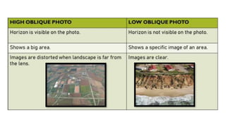
 Oblique Aerial Photographs (High vs. Low)
 Map Symbols, Keys, and Conventional Signs
 Relief Indicators: Trig Beacons, Spot Heights, and
Benchmarks
 Scale Types and Distance Measurement (Straight and
Curved)
 Area Calculation (Regular and Irregular Grid Method)
 Gradient Calculation
 Coordinate Systems: Latitude and Longitude (Degrees,
Minutes, Seconds)
 True Bearing Measurement
 Magnetic Declination and Magnetic Bearing
 Vertical Exaggeration
 General Map Reading and Interpretation
NAVIGATION CARTOGRAPHY STUDY GUIDE

Lesson Objectives:
By the end of this lesson, you should be able to:
 Calculating Exact Location (Degrees, Minutes,
Seconds)
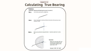
 Calculating True Bearing
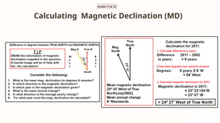
 Calculating Magnetic Declination (MD)
Analyse the spacing and pattern of contour lines
And identity various types of Landforms
To distinguish between concave/convex slopes and identify
specific landforms (e.g. ridge, spur, valley) with 100% accuracy
as demonstrated on a labelled sketch or a graded exit ticket
by the end of the lesson.
Evaluate a specific geographic scenario
Given a real‑world spatial problem (e.g., siting a new school
using multiple criteria such as slope, aspect, and proximity to
wetlands), learners will be able to evaluate the suitability of
raster and vector data for the analysis and create a simple GIS
workflow flowchart that correctly sequences at least three
data layers
Calculate real-world distances in kilometers
for various different aspects
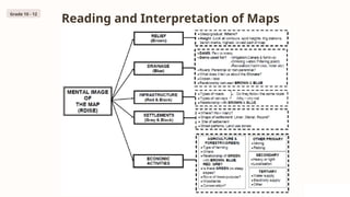
Interpret and analyse any given Map
Identifying Relief, Drainage, Infrastructure, Settlements, Map
Symbols and Economic Activities on/of both Topographic and
Orthophoto Maps. This also requires a lot of general/common
knowledge!
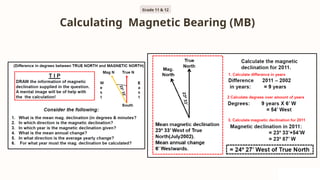
 Calculating Magnetic Bearing (MB)
 Calculating Vertical Exaggeration (VE)
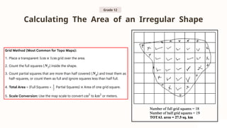
 Calculating the Area of an Irregular Shape
(Grid Method)
 Calculating Distance (Ratio, Line, Word Scale; Straight vs. Curved Features)
 Calculating Area (Regular Shapes)
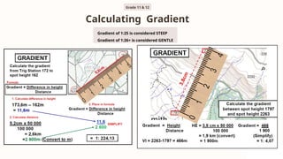
 Calculating Gradient

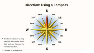
Direction: Using a Compass
 Direction is expressed by using
the points of a compass (North,
East, South and West) and the
points between them.
 There are 16 cardinal points

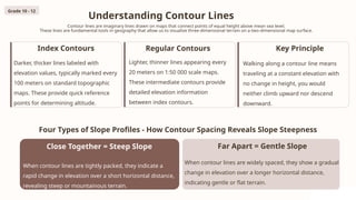
Understanding Contour Lines
Contour lines are imaginary lines drawn on maps that connect points of equal height above mean sea level.
These lines are fundamental tools in geography that allow us to visualize three-dimensional terrain on a two-dimensional map surface.
Index Contours
Darker, thicker lines labeled with
elevation values, typically marked every
100 meters on standard topographic
maps. These provide quick reference
points for determining altitude.
Regular Contours
Lighter, thinner lines appearing every
20 meters on 1:50 000 scale maps.
These intermediate contours provide
detailed elevation information
between index contours.
Key Principle
Walking along a contour line means
traveling at a constant elevation with
no change in height, you would
neither climb upward nor descend
downward.
Grade 10 - 12
Four Types of Slope Profiles - How Contour Spacing Reveals Slope Steepness
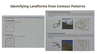
Close Together = Steep Slope
When contour lines are tightly packed, they indicate a
rapid change in elevation over a short horizontal distance,
revealing steep or mountainous terrain.
Far Apart = Gentle Slope
When contour lines are widely spaced, they show a gradual
change in elevation over a longer horizontal distance,
indicating gentle or flat terrain.

Understanding Contour Lines
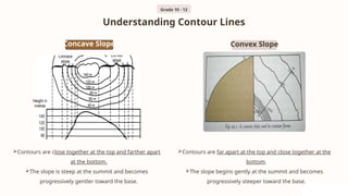
Concave Slope
Contours are close together at the top and farther apart
at the bottom.
The slope is steep at the summit and becomes
progressively gentler toward the base.
Convex Slope
Contours are far apart at the top and close together at the
bottom.
The slope begins gently at the summit and becomes
progressively steeper toward the base.
Grade 10 - 12

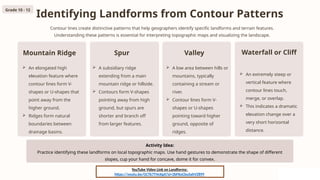
Identifying Landforms from Contour Patterns
Contour lines create distinctive patterns that help geographers identify specific landforms and terrain features.
Understanding these patterns is essential for interpreting topographic maps and visualizing the landscape.
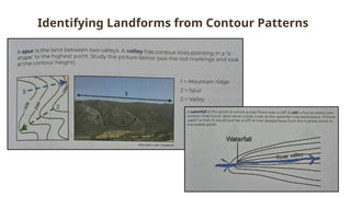
Mountain Ridge
 An elongated high
elevation feature where
contour lines form V-
shapes or U-shapes that
point away from the
higher ground.
 Ridges form natural
boundaries between
drainage basins.
Spur
 A subsidiary ridge
extending from a main
mountain ridge or hillside.
 Contours form V-shapes
pointing away from high
ground, but spurs are
shorter and branch off
from larger features.
Valley
 A low area between hills or
mountains, typically
containing a stream or
river.
 Contour lines form V-
shapes or U-shapes
pointing toward higher
ground, opposite of
ridges.
Waterfall or Cliff
 An extremely steep or
vertical feature where
contour lines touch,
merge, or overlap.
 This indicates a dramatic
elevation change over a
very short horizontal
distance.
Activity Idea:
Practice identifying these landforms on local topographic maps. Use hand gestures to demonstrate the shape of different
slopes, cup your hand for concave, dome it for convex.
YouTube Video Link on Landforms:
https://youtu.be/GCTk7T4nXgA?si=2bFKoCbuSahVZ89Y
Grade 10 - 12

Identifying Landforms from Contour Patterns

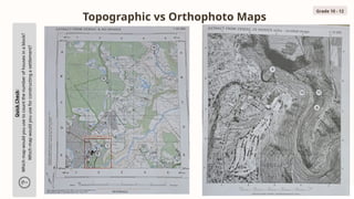
Topographic vs Orthophoto Maps
Grade 10 - 12
Quick
Check:
Which
map
would
you
use
to
count
the
number
of
houses
in
a
block?
Which
map
would
you
use
for
constructing
a
settlement?

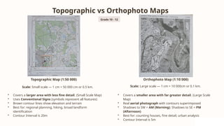
Topographic vs Orthophoto Maps
Topographic Map (1:50 000)
Scale: Small scale — 1 cm = 50 000 cm or 0.5 km.
• Covers a larger area with less fine detail. (Small Scale Map)
• Uses Conventional Signs (symbols represent all features)
• Brown contour lines show elevation and terrain
• Best for: regional planning, hiking, broad landform
identification
• Contour Interval is 20m
Orthophoto Map (1:10 000)
Scale: Large scale — 1 cm = 10 000cm or 0.1 km.
• Covers a smaller area with far greater detail. (Large Scale
Map)
• Real aerial photograph with contours superimposed
• Shadows to SW = AM (Morning); Shadows to SE = PM
(Afternoon)
• Best for: counting houses, fine detail, urban analysis
• Contour Interval is 5m
Grade 10 - 12

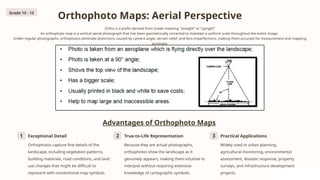
Orthophoto Maps: Aerial Perspective
Ortho is a prefix derived from Greek meaning "straight“ or "upright"
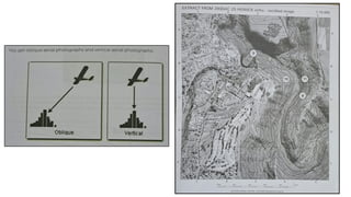
An orthophoto map is a vertical aerial photograph that has been geometrically corrected to maintain a uniform scale throughout the entire image.
Unlike regular photographs, orthophotos eliminate distortions caused by camera angle, terrain relief, and lens imperfections, making them accurate for measurement and mapping
purposes.
Advantages of Orthophoto Maps
1 Exceptional Detail
Orthophotos capture fine details of the
landscape, including vegetation patterns,
building materials, road conditions, and land
use changes that might be difficult to
represent with conventional map symbols.
2 True-to-Life Representation
Because they are actual photographs,
orthophotos show the landscape as it
genuinely appears, making them intuitive to
interpret without requiring extensive
knowledge of cartographic symbols.
3 Practical Applications
Widely used in urban planning,
agricultural monitoring, environmental
assessment, disaster response, property
surveys, and infrastructure development
projects.
Grade 10 - 12

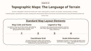
Topographic Maps: The Language of Terrain
The term "topographic" derives from Greek roots: "topo" meaning place or location, and "graphy" meaning writing or drawing.
A detailed graphic representation of a place, showing both natural physical features and human-constructed elements using standardized symbols and
contour lines.
Standard Map Layout Elements
1
Map Code and Name
Located at the top of the sheet, identifying
the specific map sheet number and
geographical area covered
2
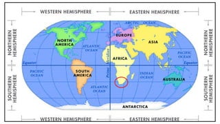
Coordinate Grid
Printed along the sides and margins,
showing latitude and longitude or grid
references for precise location
3
Legend or Key
Contains all conventional symbols used on
the map, typically located in the margin for
easy reference
4
Scale Information
Displayed as both a line scale (graphic bar)
and ratio scale (e.g., 1:50 000) for distance
calculation
Grade 10 - 12

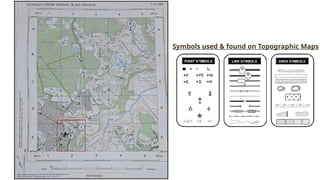
Symbols used & found on Topographic Maps

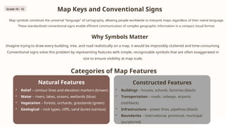
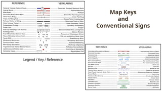
Map Keys and Conventional Signs
Map symbols constitute the universal "language" of cartography, allowing people worldwide to interpret maps regardless of their native language.
These standardized conventional signs enable efficient communication of complex geographic information in a compact visual format.
Why Symbols Matter
Imagine trying to draw every building, tree, and road realistically on a map, it would be impossibly cluttered and time-consuming.
Conventional signs solve this problem by representing features with simple, recognizable symbols that are often exaggerated in
size to ensure visibility at map scale.
Categories of Map Features
Natural Features
• Relief – contour lines and elevation markers (brown)
• Water – rivers, lakes, oceans, wetlands (blue)
• Vegetation – forests, orchards, grasslands (green)
• Geological – rock types, cliffs, sand dunes (various)
Constructed Features
• Buildings – houses, schools, factories (black)
• Transportation – roads, railways, airports
(red/black)
• Infrastructure – power lines, pipelines (black)
• Boundaries – international, provincial, municipal
(purple/red)
Grade 10 - 12

Legend / Key / Reference
Map Keys
and
Conventional Signs

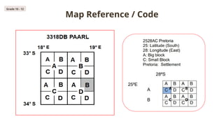
Map Reference / Code
Grade 10 - 12

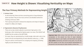
How Height is Shown: Visualizing Verticality on Maps
The Four Primary Methods for Representing Height:
• 1. Contour Lines:
◦ As we've learned, these are lines connecting points of equal elevation
above sea level. They are the most common and detailed method for
showing continuous relief.
◦ Their spacing and pattern indicate the steepness and shape of slopes (V-
shapes for valleys and ridges).
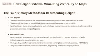
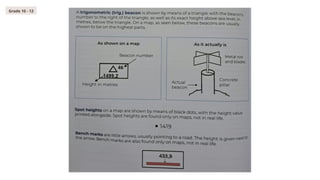
• 2. Trigonometric Beacons (Trig Beacons):
◦ These are survey markers placed on prominent high points in the
landscape, often indicating the highest peak in an area. (The HEIGHT will
ALWAYS be the number at the BOTTOM!)
◦ On maps, they are represented by a small triangle, often with a dot in the
center, and are accompanied by an exact elevation value (e.g., 1789).
△
◦ They are used as control points for surveying and mapping, providing
highly accurate elevation data.
Important Note: While contour lines exist both on the map and
conceptually on the ground (as lines of equal elevation),
trigonometric beacons, spot heights, and benchmarks are specific
map symbols representing real-world survey points. You will only
see their symbols on the map, not the physical representation on
the ground in the same way you might visualize a contour line.
Grade 10 - 12

How Height is Shown: Visualizing Verticality on Maps
The Four Primary Methods for Representing Height:
• 3. Spot Heights:
◦ These are individual points on the map where the exact elevation has been measured and recorded.
◦ They are typically shown as a small black dot with a numerical value next to it (e.g., • 850).
◦ Spot heights are found at various locations, such as hilltops, road junctions, or the bottoms of valleys, providing
precise elevation data for specific points.
• 4. Benchmarks (BM):
◦ Benchmarks are permanent survey markers, typically inscribed on rocks, concrete structures, or walls,
indicating a precise elevation above sea level.
◦ On maps, they are often represented by an arrow symbol pointing to a numerical value (e.g., BM 625.4).
↑
◦ They are used as reference points for construction, engineering, and other surveying activities.
Grade 10 - 12

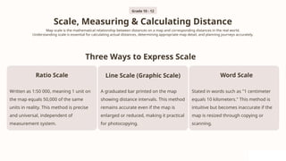
Scale, Measuring & Calculating Distance
Map scale is the mathematical relationship between distances on a map and corresponding distances in the real world.
Understanding scale is essential for calculating actual distances, determining appropriate map detail, and planning journeys accurately.
Three Ways to Express Scale
Ratio Scale
Written as 1:50 000, meaning 1 unit on
the map equals 50,000 of the same
units in reality. This method is precise
and universal, independent of
measurement system.
Line Scale (Graphic Scale)
A graduated bar printed on the map
showing distance intervals. This method
remains accurate even if the map is
enlarged or reduced, making it practical
for photocopying.
Word Scale
Stated in words such as "1 centimeter
equals 10 kilometers." This method is
intuitive but becomes inaccurate if the
map is resized through copying or
scanning.
Grade 10 - 12

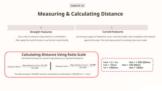
Measuring & Calculating Distance
Straight Features
Use a ruler to measure map distance in centimeters,
then apply the scale formula or use the line scale directly.
Curved Features
Use string or paper to follow the curve, mark the length, then straighten and measure
against the scale. This technique works for winding rivers and roads.
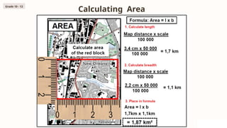
The denominator 100,000 converts centimeters to kilometers (100,000 cm = 1 km).
Use these formulas to convert map distance to real-world distance:
Calculating Distance Using Ratio Scale
Grade 10 - 12

Calculating Area
Grade 10 - 12

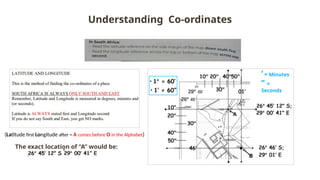
Understanding Co-ordinates
The exact location of “A” would be:
‘ = Minutes
‘’ =
Seconds
(Latitude first Longitude after = A comes before O in the Alphabet)

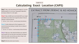
Calculating Exact Location (CAPS)
Grade 10 - 12
Step 1: Take a ruler and measure the length (3.7 cm) and
Width/breadth (3.3 cm) of your Topographic Map Block
(As shown in Block A1 on the right).
Step 2: Take a SHARP pencil and divide BOTH your length
and width of your block into 6 segments (draw 5 lines) to
indicate 10 second intervals.
 (3.7cm ÷ 6 cm = 0.6 cm - one line every 0.6cm/6mm)
Step 3: Further divide each of the 6 segments of 10
second intervals by drawing 5 smaller lines to indicate 2
second intervals.
 (3.3 cm ÷ 6 = 0.55 cm - one line every 0.55cm/5.5mm)
Step 4: Align your ruler along the feature you need the
exact location for from the top to the bottom and align it
within the smaller second lines you drew in Step 3 and
repeat the process from left to right.
Step 5: Write the entire exact location.

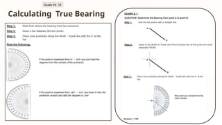
Calculating True Bearing
Grade 10 - 12

Calculating Gradient
Grade 11 & 12
Gradient of 1:25 is considered STEEP
Gradient of 1:26+ is considered GENTLE

Calculating Magnetic Declination (MD)
Grade 11 & 12

Calculating Magnetic Bearing (MB)
Grade 11 & 12

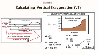
Calculating Vertical Exaggeration (VE)
50 000
2000
Grade 11 & 12

Calculating The Area of an Irregular Shape
Grade 12

Reading and Interpretation of Maps
Grade 10 - 12

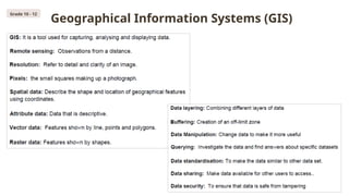
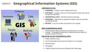
Geographical Information Systems (GIS)
Grade 10 - 12

Grade 10 - 12 Geographical Information Systems (GIS)

Geography - Mapwork Revision - Grades 10-12 - Ismail M.pptx

Mais conteúdo relacionado

Semelhante a Geography - Mapwork Revision - Grades 10-12 - Ismail M.pptx

Mais de Muzzammil Ismail

Último