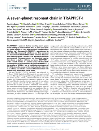
The TRAPPIST-1 system is the first transiting planet system found orbiting an ultracool dwarf star1. At least seven planets similar in radius to Earth were previously found to transit this host star2. Subsequently, TRAPPIST-1 was observed as part of the K2 mission and, with these new data, we report the measurement of an 18.77 day orbital period for the outermost transiting planet, TRAPPIST-1 h, which was previously unconstrained. This value matches our theoretical expectations based on Laplace relations3 and places TRAPPIST-1 h as the seventh member of a complex chain, with three-body resonances linking every member. We find that TRAPPIST-1 h has a radius of 0.752 R⊕ and an equilibrium temperature of 173 K. We have also measured the rotational period of the star to be 3.3 days and detected a number of flares consistent with a low-activity, middle-aged, late M dwarf.

1. 1
LETTERS
PUBLISHED: 22 MAY 2017 | VOLUME: 1 | ARTICLE NUMBER: 0129
© 2017 Macmillan Publishers Limited, part of Springer Nature. All rights reserved.
NATURE ASTRONOMY 1, 0129 (2017) | DOI: 10.1038/s41550-017-0129 | www.nature.com/nastronomy
A seven-planet resonant chain in TRAPPIST-1
Rodrigo Luger1,
​2
* , Marko Sestovic3
, Ethan Kruse1
, Simon L. Grimm3
, Brice-Olivier Demory3
,
Eric Agol1,
​2
, Emeline Bolmont4
, Daniel Fabrycky5
, Catarina S. Fernandes6
, Valérie Van Grootel6
,
Adam Burgasser7
, Michaël Gillon6
, James G. Ingalls8
, Emmanuël Jehin6
, Sean N. Raymond9
,
Franck Selsis9
, Amaury H. M. J. Triaud10
, Thomas Barclay11–
​13
, Geert Barentsen11,
​12
, Steve B. Howell11
,
Laetitia Delrez6,
​14
, Julien de Wit15
, Daniel Foreman-Mackey1
, Daniel L. Holdsworth16
,
Jérémy Leconte9
, Susan Lederer17
, Martin Turbet18
, Yaseen Almleaky19,
​20
, Zouhair Benkhaldoun21
,
Pierre Magain6
, Brett M. Morris1
, Kevin Heng3
and Didier Queloz14,
​22
The TRAPPIST-1 system is the first transiting planet system
found orbiting an ultracool dwarf star1
. At least seven plan-
ets similar in radius to Earth were previously found to transit
this host star2
. Subsequently, TRAPPIST-1 was observed as
part of the K2 mission and, with these new data, we report
the measurement of an 18.77 day orbital period for the outer-
most transiting planet, TRAPPIST-1 h, which was previously
unconstrained. This value matches our theoretical expecta-
tions based on Laplace relations3
and places TRAPPIST-1 h
as the seventh member of a complex chain, with three-body
resonances linking every member. We find that TRAPPIST-1 h
has a radius of 0.752 R⊕ and an equilibrium temperature of
173 K. We have also measured the rotational period of the star
to be 3.3 days and detected a number of flares consistent with
a low-activity, middle-aged, late M dwarf.
The star TRAPPIST-1 (EPIC 246199087) was observed for
79 days by NASA’s Kepler Space Telescope in its two-reaction wheel
mission4
(K2) as part of Campaign 12, starting on 2016 December 15
and ending on 2017 March 4. The spacecraft was in safe mode
between 2017 February 1 and 2017 February 6, resulting in a five-
day loss of data. On downlink from the spacecraft, the raw cadence
data are typically calibrated with the Kepler pipeline5
, a lengthy
procedure that includes background subtraction, smear removal,
and undershoot and non-linearity corrections. However, given the
unique science drivers in this dataset, the raw, uncalibrated data for
Campaign 12 were made publicly available on 2017 March 8, shortly
after downlink. We download and calibrate the long cadence (expo-
sure time texp =​ 30 min) and short cadence (texp =​ 1 min) light curves
using a simple column-by-column background subtraction, which
also removes smear and dark noise (see Methods). Because of its
two failed reaction wheels, the rolling motion of the Kepler space-
craft due to torque imbalances introduces strong instrumental sig-
nals, leading to an increase in photometric noise by a factor of about
three to five compared with the original mission. As TRAPPIST-1 is
a faint M8 dwarf with Kepler magnitude Kp ≈​ 16–17 (see Methods),
these instrumental signals must be carefully removed to reach the
~0.1% relative photometric precision required to detect Earth-size
transits6
. To this end, we detrend the long cadence light curve for
TRAPPIST-1 using both EVEREST7,8
and a Gaussian process-
based pipeline, achieving an average 6 h photometric precision of
281.3 ppm, a factor of three improvement over the raw light curve.
After analysis of the long cadence light curve, we detrend the short
cadence light curve in the vicinity of the features of interest, achiev-
ing a comparable or higher 6 h precision (see Methods).
We conduct three separate transit searches on the long cadence
light curve, aiming to constrain the period of TRAPPIST-1 h,
which had only been observed to transit once2
, and to detect addi-
tional planets in the system. A dynamical analysis made by our
team before the release of the K2 data suggested certain values of
the period of TRAPPIST-1 h based on the presence of three-body
resonances among the planets. Three-body resonances satisfy
− + + ≈− − −
pP p q P qP( ) 01
1
2
1
3
1
and pλ1−​(p +​ q)λ2 +​ qλ3 =​ ϕ for inte-
gers p and q where Pi and λi are the period and mean longitude of
the ith planet9,10
and ϕ is the three-body angle, which librates about
a fixed value. Such resonances occur both in our Solar System—
the archetypical case being the Laplace resonance among Jupiter’s
1
Astronomy Department, University of Washington, Seattle, Washington 98195, USA. 2
NASA Astrobiology Institute’s Virtual Planetary Laboratory,
Seattle, Washington 98195, USA. 3
University of Bern, Center for Space and Habitability, Sidlerstrasse 5, CH-3012 Bern, Switzerland. 4
Laboratoire AIM
Paris-Saclay, CEA/DRF–CNRS–Université Paris Diderot, IRFU/SAp Centre de Saclay, 91191 Gif-sur-Yvette, France. 5
Department of Astronomy and
Astrophysics, University of Chicago, 5640 South Ellis Avenue, Chicago, Illinois 60637, USA. 6
Space Sciences, Technologies and Astrophysics Research
Institute, Université de Liège, Allée du 6 Août 19C, B-4000 Liège, Belgium. 7
Center for Astrophysics and Space Science, University of California
San Diego, La Jolla, California 92093, USA. 8
IPAC, Mail Code 314-6, California Institute of Technology, 1200 East California Boulevard, Pasadena,
California 91125, USA. 9
Laboratoire d’Astrophysique de Bordeaux, Université Bordeaux, CNRS, B18N, allée Geoffroy Saint-Hilaire, 33615 Pessac, France.
10
Institute of Astronomy, Madingley Road, Cambridge CB3 0HA, UK. 11
NASA Ames Research Center, Moffett Field, California 94043, USA. 12
Bay Area
Environmental Research Institute, 25 2nd Street Ste 209 Petaluma, California 94952, USA. 13
NASA Goddard Space Flight Center, Greenbelt, Maryland
20771, USA. 14
Cavendish Laboratory, J.J. Thomson Avenue, Cambridge CB3 0HE, UK. 15
Department of Earth, Atmospheric and Planetary Sciences,
Massachusetts Institute of Technology, 77 Massachusetts Avenue, Cambridge, Massachusetts 02139, USA. 16
Jeremiah Horrocks Institute, University of
Central Lancashire, Preston PR1 2HE, UK. 17
NASA Johnson Space Center, 2101 NASA Parkway, Houston, Texas 77058, USA. 18
Laboratoire de Météorologie
Dynamique, Sorbonne Universités, UPMC Université Paris 06, CNRS, 4 place Jussieu, 75005 Paris, France. 19
Space and Astronomy Department, Faculty of
Science, King Abdulaziz University, 21589 Jeddah, Saudi Arabia. 20
King Abdullah Centre for Crescent Observations and Astronomy, Makkah Clock, Mecca
24231, Saudia Arabia. 21
LPHEA Laboratory, Oukaïmeden Observatory, Cadi Ayyad University FSSM, BP 2390 Marrakesh, Morocco. 22
Observatoire de
Genève, Université de Genève, 51 chemin des Maillettes, CH-1290 Sauverny, Switzerland. *e-mail: rodluger@uw.edu

2. 2
© 2017 Macmillan Publishers Limited, part of Springer Nature. All rights reserved.
NATURE ASTRONOMY 1, 0129 (2017) | DOI: 10.1038/s41550-017-0129 | www.nature.com/nastronomy
LETTERS NATURE ASTRONOMY
satellites, satisfying (p, q) =​ (1, 2)—and in exoplanet systems, two
of which were recently observed to have resonant chains among
four planets: Kepler-22311
with (p, q) =​ (1, 1) and Kepler-8012
with
(p, q) =​ (2, 3). Among the inner six planets in TRAPPIST-1, there
are four adjacent sets of three planets that satisfy this relation for
1 ≤​ p ≤​ 2 and 1 ≤​ q ≤​ 3 (Table 1). This suggested that the period of
planet TRAPPIST-1 h may also satisfy a three-body resonance with
TRAPPIST-1 f and g. The six potential periods of TRAPPIST-1 h
that satisfy three-body relations with 1 ≤​ p, q ≤​ 3 are 18.766 days
(p =​ q =​ 1), 14.899 days (p =​ 1, q =​ 2), 39.026 days (p =​ 2, q =​ 1),
15.998 days (p =​ 2, q =​ 3), 13.941 days (p =​ 1, q =​ 3) and 25.345
days (p =​ 3, q =​ 2). We examined ~1,000 h of ground-based data
taken before the Spitzer dataset2
and found a lack of obvious addi-
tional transits at the expected times for all these periods apart from
18.766 days. The period of 18.766 days corresponds to prior transit
times in windows that were missed by the previous ground-based
campaigns, hence this was the only period that could not be ruled
out. As this value is consistent with the period estimate of −
+
20 6
15
day
based on the duration of the Spitzer transit, we had reason to believe
that it was the correct period for TRAPPIST-1 h. To test this hypoth-
esis, in our first transit search we simply fold the long cadence light
curve at the four expected times of transit given this period and the
single Spitzer transit time, finding evidence for a transiting planet
with that period. Follow-up with detrended short cadence data con-
firms the transit-like shape of each of the four events and a depth
consistent with that of TRAPPIST-1 h (see Methods).
To prove the uniqueness of this detection, in a second analysis
we search the detrended K2 light curve after subtracting a transit
model including all known transits of planets TRAPPIST-1 b–g,
based on published ephemerides and planet parameters2
. We use the
photometric residuals as input to a box-fitting least-squares (BLS)
algorithm (see Methods) to search for additional transit signals. In
this search, we do not impose prior information on TRAPPIST-1 h.
We find a periodic signal at ~18.77 days with a transit centre at
Barycentric Julian date (BJD) =​ 2,457,756.39, which matches the
single transit observed by Spitzer2
.
Independently, we perform a joint instrumental–transit model
fit to the data after subtracting a model for planets TRAPPIST-1 b–g
based on the Spitzer parameters (see Methods). We compute the rela-
tive likelihood (Δ​χ​2
) of a transit model with the best-fit Spitzer param-
eters of TRAPPIST-1 h centred at every long cadence and sum the
Δ​χ​2
values at the transit times corresponding to different periods in
the range 1–50 days. Strong peaks emerge at 18.766 days and its aliases,
corresponding to four transit-like events consistent with the param-
eters of TRAPPIST-1 h at the times recovered in the previous searches.
We use the orbital period of TRAPPIST-1 h determined in the
previous step along with the parameters2
of planets TRAPPIST-1 b–g
to determine whether a model including TRAPPIST-1 h is favoured.
This is achieved through Markov Chain Monte Carlo (MCMC)
model fits with and without TRAPPIST-1 h. We find a Bayes
factor of 90 in favour of a model that includes TRAPPIST-1 h (see
Methods), supporting the photometric detection of this seventh
planet in the K2 dataset. The detection of TRAPPIST-1 h is thus
supported by: (1) the three transit search analyses that recovered
both the orbital phase from the Spitzer ephemeris2
and the period
of 18.766 days; (2) the Bayes factor in favour of the seven-planet
model; and (3) the orbital period that is the exact value predicted
by Laplace relations. Figure 1 shows the full light curve, the newly
found transits of TRAPPIST-1 h and an update to the geometry of
the orbits given the new orbital period. Table 2 reports the proper-
ties of the planet derived in this study.
To characterize the three-body resonance, we use the transit tim-
ing data to identify ϕ (see Methods) for each set of three planets.
A full transit timing cycle has not elapsed within the data, so we
cannot estimate the libration centre for each value of ϕ. However,
we report in Table 1 the values of ϕ represented in the dataset.
InthecaseofJupiter’ssatellites,ϕ =​ 180°,butduetothecomplexityof
this multi-planet system, we make no prediction for TRAPPIST-1 at
this time. Migration and damping simulations applied to Kepler-80
(ref. 12
) naturally predicted the values of the libration centres in that
system; the measured values for TRAPPIST-1 b–h call for future
theoretical work to interpret.
The resonant structure of the system suggests that orbital migra-
tion may have played a part in its formation. Embedded in gaseous
planet-forming disks, planets growing above ~0.1 M⊕ (approxi-
mately the mass of Mars) create density perturbations that torque
the planets’ orbits and trigger radial migration13
. One model for the
origin of low-mass planets found very close to their stars proposes
that Mars- to Earth-sized planetary embryos form far from their
stars and then migrate inwards14
. The inner edge of the disk pro-
vides a migration barrier15
such that the planets pile up into chains
of mean motion resonances16–18
. This model matches the observed
period ratio distribution of adjacent low-mass (≲10 M⊕) planets19
if the majority (~90%) of resonant chains become unstable and
undergo a phase of giant impacts20
. Some resonant chains do sur-
vive and a handful of systems with multiple resonances among low-
mass planets have been characterized11,21
. The TRAPPIST-1 system
may thus represent a pristine surviving chain of mean motion res-
onances. Given that the planet-forming disk of TRAPPIST-1 was
probably low in mass22
and the planets themselves are low mass,
their migration was probably relatively slow. This may explain why
the resonant chain of TRAPPIST-1 is modestly less compact than
chains in systems with more massive planets11,20,21
; this may have
protected the chain from instability23
.
Tidal interactions are likely to be important in the planets’ orbital
evolution, given how close the planets orbit TRAPPIST-124
. Tidal sim-
ulations of the system (see Methods) show that the eccentricity of each
planet is damped to <​0.01 within a few million years. Nonetheless,
tidal heating is significant: all planets except TRAPPIST-1 f, g and h
have a tidal heat flux higher than Earth’s total heat flux.
The incident stellar flux on planet TRAPPIST-1 h, 200 W m−2
, is
less than the 300 W m−2
required to sustain surface liquid water under
an N2/CO2/H2O atmosphere (see Methods). To obtain the missing
100 W m−2
from tidal heating would require a high eccentricity, which
is strictly incompatible with the orbits of the other planets. Our simula-
tions show that the stellar input is also too low to sustain a thick CO2
atmosphere due to CO2 condensation. In particular, CO2 levels cannot
exceed 100 ppm within a 1 bar N2 atmosphere. Alternatively, a liquid
water ocean is possible under a layer of ice. The minimum thickness h
of this layer of ice depends on the internal heat flux ϕint:






ϕ
≈ −
−
h 250
1 W m
mint
2
1
Assuming the Earth’s current geothermal flux of 0.090 W m−2
, a
layer of ice 2.8 km thick (the mean depth of Earth’s oceans) would
be necessary.
Table 1 | Three-body resonances of TRAPPIST-1.
Planets 1, 2, 3 p q − +
+ −
(day )
p
P
p q
P
q
P
( ) 1
1 2 3
ϕ λ λ λ= − + +p p q q( )1 2 3
b, c, d 2 3 (−​4.6, −​0.3) ×​ 10−5
(176°, 178°)
c, d, e 1 2 (−​5.2, +​ 4.5) ×​ 10−5
(47°, 50°)
d, e, f 2 3 (−​1.9, +​ 1.9) ×​ 10−4
(−​154°, −​142°)
e, f, g 1 2 (−​1.4, +​ 1.1) ×​ 10−4
(−​79°, −​72°)
f, g, h 1 1 (−​6.0, +​ 0.2) ×​ 10−5
(176.5°, 177.5°)
The transit times are used to track the ϕ angles of each set of three adjacent planets over
the dataset, assuming low eccentricities such that transits occur at a phase angle λ =​ 90°11
.
The ranges of three-body frequency and angle given encompass the changes—most likely
librations—seen during the observations.

3. 3
© 2017 Macmillan Publishers Limited, part of Springer Nature. All rights reserved.
NATURE ASTRONOMY 1, 0129 (2017) | DOI: 10.1038/s41550-017-0129 | www.nature.com/nastronomy
LETTERSNATURE ASTRONOMY
(0.26 day−1
for peak fluxes >​1% of the continuum, 40 times less
frequent than active M6–M9 dwarfs29
) are consistent with a low-
activity M8 star, also arguing in favour of a relatively old system. An
energetic flare erupted near the end of the K2 Campaign and was
observed by Kepler. Full modelling of flares will be presented in a
forthcoming paper.
The K2 observations of the TRAPPIST-1 star have enabled the
detection of the orbital period of TRAPPIST-1 h, continuing the
pattern of Laplace resonances among adjacent triplets of planets.
We search for, but do not detect, additional planets in the system.
Compared with previous ground-based and Spitzer observations,
the continuous coverage, high precision and shorter wavelength
of the K2 observations enable a robust estimate of the rotational
Although the long spin-down times of ultracool dwarfs prevent
the derivation of a robust gyrochronology relation25
, the rotational
period of TRAPPIST-1 can be used to derive a provisional age
estimate for the system. Fourier analysis of the detrended K2 data
(Fig. 2), which is visibly modulated by star spots, leads to the deter-
mination of a rotational period of ~3.3 days for the host star (see
Methods). This rotation corresponds to an angular momentum of
~1% of that of the Sun. It is roughly in the middle of the period dis-
tribution of nearby late M dwarfs26
, suggesting an age in the range
3–8 Gyr based on a star formation rate that decreases slightly over
time27
. Such an age is consistent with the star’s solar metallicity1
and
borderline thin disk–thick disk kinematics28
. The amplitude of the
modulation due to star spots and infrequent weak optical flares
70605040
0.985
0.990
0.995
1.000
1.005
a
b
c d
1101009080
0.985
0.990
0.995
1.000
1.005
–0.05 0.00 0.05
0.90
0.92
0.94
0.96
0.98
1.00
–0.06 –0.04 –0.02 0.00 0.02 0.04 0.06
–0.06
–0.04
–0.02
0.00
0.02
0.04
0.06
K2 long cadence data
Barycentric Julian date – 2,457,700 (day)
RelativebrightnessRelativebrightness
K2 in safe mode
1b 1c 1d 1e 1f 1g 1h
1b 1c 1d 1e 1f 1g 1h
Time from mid–transit (day)
Relativebrightness
Transit 1
Transit 2
Transit 3
Transit 4
Folded lightcurve
Orbital separation (au)
Figure 1 | Long cadence K2 light curve of TRAPPIST-1 detrended with EVEREST. a, The first half of the detrended K2 light curve with stellar variability
removed via LOESS regression (order =​ 1; width =​ 0.15 day). Data points are in black and our highest likelihood transit model for all seven planets is plotted
in thin grey. Coloured diamonds indicate which transit belongs to which planet. Two transits of TRAPPIST-1 h are observed (light blue diamonds). b, The
second half of the detrended K2 light curve. Two additional transits of TRAPPIST-1 h are visible. c, The top four curves show the detrended and whitened
short cadence in light blue, with a transit model based on the Spitzer parameters in dark blue. Binned data is over-plotted in white for clarity. The folded
light curve is displayed at the bottom. d, View from above (observer to the right) of the TRAPPIST-1 system at the date when the first transit was obtained
for this system. The grey region is the surface liquid water habitable zone.

4. 4
© 2017 Macmillan Publishers Limited, part of Springer Nature. All rights reserved.
NATURE ASTRONOMY 1, 0129 (2017) | DOI: 10.1038/s41550-017-0129 | www.nature.com/nastronomy
LETTERS NATURE ASTRONOMY
period and flare activity of the star, motivating further study of the
atmospheres and dynamical evolution of the planetary system.
Methods
Light curve preparation. We use the package kadenza to generate a target pixel
file from the Campaign 12 raw data for TRAPPIST-1 (see Code availability).
In addition to EPIC ID 246199087, which corresponds to a standard-size postage
stamp centred on TRAPPIST-1, the Kepler GO Office also made available a larger,
11 ×​ 11 pixel custom mask with a different ID (200164267), which we use for the
purposes of this study. We manually select a rectangular 6 ×​ 6 pixel (24′​′​ ×​ 24′​′​)
aperture centred on TRAPPIST-1 and use the median values of the remaining
pixels to perform a column-by-column background subtraction. This process
removes dark current and background sky signals while mitigating smear due to
bright stars in the same CCD column as the target. Based on simple error function
fits to the stellar image, we find that our aperture encloses >​0.9996 of the flux of
TRAPPIST-1 h throughout the entire time series. We then detrend and perform
photometry on the pixel level data using two independent pipelines: EVEREST and
a Gaussian process based detrender. For computational expediency, we perform
preliminary analyses on the long cadence data, following up on features of interest
in the short cadence data.
Light curve detrending using EVEREST. The EVEREST K2 pipeline7
uses
a variant of pixel level decorrelation30
(PLD) to remove instrumental systematics
from stellar light curves. Given a stellar image spread out over a set of
pixels p{ }i , EVEREST regresses on polynomial functions of the fractional pixel
fluxes, Σp p/i j j
, identifying the linear combination of these that best fits the
instrumental signals present in the light curve. Because astrophysical signals
(such as transits) are equally present in each of the pixels, whereas instrumental
signals are spatially variable, PLD excels at removing instrumental noise while
preserving astrophysical information. EVEREST uses a Gaussian process to
model correlated astrophysical noise and uses an L2-regularized regression
scheme to minimize overfitting.
As PLD may overfit in the presence of bright contaminant sources in the target
aperture7
, we manually inspect the TRAPPIST-1 K2 postage stamp and high-
resolution images of TRAPPIST-1 taken with the Apache Point Observatory ARC
3.5 m telescope in the Slone Digital Sky Survey z band to verify that there is no
other target brighter than the background level in our adopted aperture, consistent
with results obtained from Gemini-South speckle imaging of the target31
. Given
the faint magnitude of TRAPPIST-1 in the Kepler band, we use the PLD vectors of
14 nearby bright stars (EPIC IDs 246177238, 246165150, 246211745, 246171759,
246127507, 246228828, 206392586, 246121678, 246229336, 246196866, 24621755,
246239441 and 246144695), generated using the same method, to improve the
signal-to-noise ratio of the instrumental model8
. We further mask the data
in the vicinity of all transits of planets TRAPPIST-1 b–g and the potential transits
of TRAPPIST-1 h when computing the model to prevent transit overfitting.
We then divide the light curve into three roughly equal segments and detrend each
separately to improve the predictive power of the model. Following these steps, we
obtain a detrended light curve for TRAPPIST-1 with a 6 h photometric precision7,32
of 281.3 ppm, a factor of three improvement on that of the raw light curve
(884.4 ppm); see Fig. 1. Before the K2 observation, we estimated the Kp magnitude
of TRAPPIST-1 to be 17.2 ±​ 0.3 based on a fit to a corrected blackbody spectrum.
However, the photometric precision we achieve with EVEREST is inconsistent
with a target dimmer than Kp ≈​ 17. Our detrending therefore suggests that the
magnitude of TRAPPIST-1 in the Kepler band is 16 <​ Kp <​ 17.
Light curve detrending using Gaussian process model. Independently, we also
detrend the data with a Gaussian process-based pipeline. To perform aperture
photometry, we locate the star using a centroid fit and apply a circular top-hat
aperture following the star’s centroid coordinates. We then use a Gaussian process
model to remove the pointing drift systematics using an additive kernel with
separate spatial, time and white noise components33,34
:










= −
−
−
−
k x y x y A
x x
L
y y
L
( , , , ) exp
( ) ( )
(1)xy i i j j xy
i j
x
i j
y
2
2
2
2










= −
−
k t t A
t t
L
( , ) exp
( )
(2)xy i j t
i j
t
2
2
σ δ= + +K k x y x y k t t( , , , ) ( , ) (3)ij xy i i j j t i j ij
2
where x and y are the pixel coordinates of the centroid, t is the time of the
observation, δij is the Kronecker delta and the other variables (amplitudes
Axy and At, length scales Lx and Ly, timescale Lt and standard deviation σ) are
hyperparameters of the Gaussian process model. We use the GEORGE package35
in PYTHON to implement the Gaussian process model. To find the maximum
likelihood hyperparameters, we use a differential evolution algorithm36
followed by
a local optimization. This method was tested on magnitude 16–18 stars
observed in Campaign 10 of K2 and we use the results of those tests, and of
previous Gaussian process applications to K2 data34
, to inform our priors
on the hyperparameters.
For the TRAPPIST-1 data, we use an iterative σ-clipping method to
remove outliers and prevent the time component from overfitting. This method
has been previously used in the k2sc (ref. 34
) pipeline. First, using fiducial
hyperparameter values based on the analysis of a Campaign 10 target, we remove
all measurements with residuals >​3σ from the mean Gaussian process prediction.
With the remaining measurements, we update the hyperparameters by
maximizing the Gaussian process likelihood. Using these parameters, we once
again clip all 3σ outliers and maximize the Gaussian process likelihood using
only the remaining measurements. The final detrending is calculated for all
points, including outliers.
Photometric analysis I. We fold the long cadence data on the dynamically
predicted orbital period of 18.765 days for TRAPPIST-1 h with a time of first
transit constrained by the Spitzer observation, revealing a feature consistent
with a transit in both the EVEREST- and Gaussian process-based light curves.
To confirm the planetary nature of this signal, we analyse the short cadence
data. To this end, we use kadenza to generate a short cadence target pixel file of
TRAPPIST-1 and detrend it in windows of 1.5–2.0 days centred on each of the
four features using EVEREST. We use the PLD vectors of five bright stars observed
in short cadence mode (EPIC IDs 245919787, 246011640, 246329409, 246331757
and 246375295) to aid in the detrending. When generating these light curves,
we explicitly mask large flares so that these do not inform the fit. Following this
procedure, we obtain binned 6 h photometric precisions of 266.6, 176.1, 243.4 and
219.3 ppm in each of the four windows. The short and long cadence data in these
windows is shown in Supplementary Fig. 1. Additional correction of the light
curve is necessary for transits 3 and 4 because the transit of TRAPPIST-1 h
coincides with a transit of TRAPPIST-1 b (panel 3a of Supplementary Fig. 1) and a
small flare (panel 4b). The transit of TRAPPIST-1 b is subtracted out using a transit
model37
with the Spitzer parameters and a mid-transit time determined from the
data, yielding the light curve in panel 3b. The flare is fitted using a three-parameter
flare model38
for stars observed with Kepler, yielding the light curve in panel 4b
(see also Supplementary Fig. 2). In both cases, the transit of TRAPPIST-1 h is
visible in the residuals. In Supplementary Fig. 3 we show the folded short cadence
data after accounting for transit timing variations (TTVs), with a transit model
based solely on the Spitzer parameters.
Photometric analysis II. We use the long cadence detrended light curve to perform
a transit search with a BLS39
. We set the BLS to orbital periods ranging from
Table 2 | Properties of TRAPPIST-1 h, limb-darkening parameters
and transit timings derived using a joint Spitzer and K2 dataset.
Parameter Value
Transit depth, (Rp/R
*
)2
(%) 0.346 ±​ 0.018
Transit duration (day) 0.0525 ±​ 0.0008
Impact parameter, b (R
*
) −
+
0.45 0.08
0.06
Mid-transit time, T0 (BJDTDB) 2,457,662.55284 ±​ 0.00037
Period, P (day) −
+
18.767 0.003
0.004
Radius ratio, Rp/R
*
0.0588 ±​ 0.0016
Radius, Rp (R⊕) −
+
0.752 0.031
0.032
Inclination, i (°) −
+
89.76 0.04
0.05
Scale parameter, a/R
*
109 ±​ 4
Equilibrium temperature (K) 173 ±​ 4
Irradiation, Sp (S⊕) 0.165 ±​ 0.025
Limb-darkening parameters (Kepler bandpass)
u1 1.00 ±​ 0.02
u2 −0.04 ±​ 0.04
Individual transit timings from K2 (BJDTDB)
Transit 1 −
+
2,457,756.3874 0.0013
0.0013
Transit 2 −
+
2,457,775.1539 0.0016
0.0016
Transit 3 −
+
2,457,793.9230 0.0025
0.0024
Transit 4 −
+
2,457,812.6987 0.0042
0.0045
Parameter values are the medians of the posterior distributions from the MCMC and the
associated errors are the 1σ credible intervals. Rp is the planet radius and a is the semimajor axis.

5. 5
© 2017 Macmillan Publishers Limited, part of Springer Nature. All rights reserved.
NATURE ASTRONOMY 1, 0129 (2017) | DOI: 10.1038/s41550-017-0129 | www.nature.com/nastronomy
LETTERSNATURE ASTRONOMY
10 to 50 days. The ratio of the transit duration over the planet orbital period is set
between 0.0007 and 0.06 to include a wide range of orbital periods, eccentricities
and impact parameters for additional planets in the system. As a result of Kepler’s
30 minute cadence, transits of planets orbiting TRAPPIST-1 appear significantly
smeared out, which we take into account in our analysis. The highest peak in the
periodogram corresponds to a signal with a 15.44 day period. Its origin stems
from residuals in blended transits with TRAPPIST-1 c and d and from one outlier
in the data. No signal is seen at the two other epochs where a transit should
have appeared, which confirms the signal is spurious. The next highest peak
in the periodogram corresponds to a ~18.77 day period and a transit centre at
BJD =​ 2,457,756.39, which is consistent with the single transit seen with Spitzer.
We then use an MCMC algorithm40
to derive the transit parameters of
TRAPPIST-1 h from the detrended light curve. Each photometric data point is
attached to a conservative error bar that accounts for the uncertainties in the
detrending process presented in the previous section. We impose normal priors in
the MCMC fit on the orbital period, transit mid-time centre and impact parameter
for planets TRAPPIST-1 b–g to the values recently published2
. We further assume
circular orbits for all planets1,2
. We also include normal priors for the stellar
properties, which are 𝒩(0.080, 0.0072
) M⊙ for the mass, 𝒩(0.117, 0.0042
) R⊙ for
the radius, 𝒩(2,555, 852
) K for the effective temperature and 𝒩(0.04, 0.082
) dex
for the metallicity2
. We use these stellar parameters to compute the quadratic limb-
darkening coefficients u1 and u2 in the Kepler bandpass from theoretical tables41
. In a
first MCMC fit, we use a seven-planet model that includes all seven planets, with no
prior information on the orbital period or t0 (the time of transit) of TRAPPIST-1 h.
In the second fit we use a six-planet model that excludes TRAPPIST-1 h.
We use the results from both MCMC fits to compute the Bayesian and Akaike
information criteria to determine which model is favoured. We find Bayesian
information criteria values of 2,888 and 2,897 for the seven- and six-planet models,
respectively. This corresponds to a Bayes factor =−e 90BIC BIC( )/21 2 in favour of the
seven-planet model. Similarly, we find Akaike information criterion values of 2,691
and 2,725 for the seven- and six-planet models, respectively. We perform a third
MCMC fit to refine the transit parameters of TRAPPIST-1 h. For this fit,
we use as input data the K2 short cadence data centred on the four transits
of TRAPPIST-1 h (Fig. 1) and the single transit light curve previously obtained
with Spitzer. This fit includes a model for TRAPPIST-1 b and a flare that both
affect the transit shape of TRAPPIST-1 h in the K2 short cadence data. This fit
also allows for TTVs for the individual transit timings. We find photometric
precisions of 365 and ~1,100 ppm per 10 minutes for the Spitzer and K2 data,
respectively. We report the median and 1σ credible intervals of the posterior
distribution functions for the transit parameters of TRAPPIST-1 h in Table 2,
along with the individual transit times.
Photometric analysis III. To prevent the overfitting of transit features, we
mask all transits of planets TRAPPIST-1 b–h when detrending with EVEREST.
However, this inevitably results in a lower detrending power during transits.
A powerful alternative to this detrend-then-search method is to simultaneously fit
the instrumental and transit signals without masking these features42
. We therefore
conduct a second separate blind search on the EVEREST light curve specifically for
TRAPPIST-1 h. Given a raw light curve y, a data covariance matrix Σ​and a single
transit model mt0 centred at t =​ t0, the log likelihood of the transit fit is
L Σ= − − − +⊺ −
Cy m y mlog
1
2
( ) ( ) (4)t t
1
0 0
where C is a constant. The data covariance matrix, Σ​, is the sum of the astrophysical
covariance and the L2-regularized PLD covariance and is given by
Σ Λ Κ= +⊺X X (5)
where Κ​is the astrophysical covariance given by the EVEREST Gaussian process
model, X is the matrix of PLD regressors (the design matrix), and Λ​is the prior
covariance of the PLD weights (the regularization matrix), which we obtain by
cross-validation8
. As the transit shape and the duration of TRAPPIST-1 h are
known2
, the only free parameter in the search is t0, the time of transit. We therefore
evaluate mt0 multiple times, centering the transit model at each long cadence and
computing the likelihood of the transit model fit as a function of cadence number.
We then subtract these values from the log likelihood of the data with no transit
model ( =m 0t0 ) and multiply by 2 to obtain the Δ​χ​2
metric, which measures the
decrease in the χ​2
value of the fitted light curve for a transit of TRAPPIST-1 h
centred at each cadence. We also compute Δ​χ​2
conditioned on the known ‘true’
transit depth of TRAPPIST-1 h, d0 =​ 0.00352 ±​ 0.000326:





Δχ Δχ
σ
= −
−d d
(6)
d
cond
2 2 0
2
where
σ Σ= ⊺ −d m y (7)d t
12
0
is the maximum likelihood depth of the transit model and
σ Σ= ⊺ − −
( )m m (8)d t t
12 1
0 0
is the variance of the depth estimate. Positive peaks in Δ​χ​2
indicate features that are
well described by the transit model, whereas positive peaks in Δχcond
2
reveal features
that are well described by the transit model with depth d =​ d0. In Supplementary
40 80 100
1
2
a
b
60Relativeflux
40 60 80 100
Barycentric Julian date – 2457700.00 (day)
0.98
0.99
1.00
1.01
1.02
Relativeflux
b b b b b b b b b b b b b b b b b b b b b b b b b b b b b b b b b b b b b b b b b b b b b b b b b b b b b
c c c c c c c c c c c c c c c c c c c c c c c c c c c c c c c c c
d d d d d d d d d d d d d d d d d d d d
e e e e e e e e e e e e e
f f f f f f f f
g g g g g g g
hhhh
Figure 2 | Entire systematics-corrected K2 dataset with low-frequency trends removed. The stellar rotation is apparent in the peaks and troughs of the
variability, as are the flares, which, in some cases, appear as single spikes. The planet transits are marked. a, Full dynamic range of the curve, including an
extreme event at approximately day 113. b, Zoomed view of the region outlined in grey in a.

6. 6
© 2017 Macmillan Publishers Limited, part of Springer Nature. All rights reserved.
NATURE ASTRONOMY 1, 0129 (2017) | DOI: 10.1038/s41550-017-0129 | www.nature.com/nastronomy
LETTERS NATURE ASTRONOMY
Fig. 4, we show the two Δ​χ​2
metrics across the full TRAPPIST-1 light curve after
subtracting a transit model for planets TRAPPIST-1 b–g based on their Spitzer
parameters. The strongest features in the Δ​χ​2
plot are flares because these can be
fitted out with an inverted transit model. When conditioning on the true depth of
TRAPPIST-1 h, the significance of most of the flare features decreases, revealing
the four peaks of TRAPPIST-1 h.
To assess the robustness of our detection, we compute the total Δχcond
2
as a
function of orbital period. Starting from the time of transit of TRAPPIST-1 h in the
Spitzer dataset, we compute the times of transit in the K2 light curve for 500,000
values of the orbital period evenly spaced between 1 and 50 days and sum the
values of Δχcond
2
at each transit time to produce the total ΔχP
2
. We sum these in
two different ways. First, we linearly interpolate the grid of Δχcond
2
to each transit
time to obtain ΔχP
2
for perfectly periodic transits. Next, to allow for TTVs of up to
1 h, we take the largest value of Δχcond
2
in the vicinity of each transit time and sum
them for each period. We adopted a tolerance of two cadences, corresponding to
maximum TTVs of 1 h. Our results are shown in Supplementary Fig. 5, where we
plot the periodic ΔχP
2
and the ΔχP
2
allowing for TTVs. In both cases, the period of
TRAPPIST-1 h (18.766 days) and its one-half and one-third period aliases emerge
as the three strongest peaks. The peak at 18.766 days is the strongest signal
in the period range constrained by the Spitzer transit2
and confirms our detection
of TRAPPIST-1 h.
Three-body angles. The mean longitude of a planet with orbital period P is an
angular variable that progresses at a constant rate with respect to time t, which is
measured from the time the planet passes a given reference direction:
λ =
∘
P
t
360
(9)
with λ measured in degrees. For transiting planets, the reference direction is
taken as the plane perpendicular to the observer’s line of sight as the planet is
progressing towards the transiting configuration. We assume orbits with negligible
eccentricities11
, for which λ​ =​ 90° at transit mid-time, so that we may write:






λ = ° +
−t T
P
360
1
4
(10)n
for each planet, where Tn is the time of transit of the nth planet. For a three-body
resonance (p, q), we may therefore express the three-body angle as:








ϕ= ° − + + − + − + +p
T
P
p q
T
P
q
T
P
p
t
P
p q
t
P
q
t
P
360 ( ) ( ) (11)1
1
2
2
3
3 1 2 3
The state of a ϕ value is assessed when the individual transit times of
three planets are taken near each other. For instance, for the transit times2
Tf =​ 7,662.18747, Tg =​ 7,665.35151, Th =​ 7,662.55463 and (p, q) =​ (1, 1), we
compute ϕ =​ 177.4° at t =​ 7,664 (BJD −​2,450,000).
Tidal simulations. Tidal interactions with the star are important for all seven
planets. We perform N-body simulations of the system, including an equilibrium
tidal dissipation formalism43,44
using the Mercury-T code45
. We use orbital
parameters from the discovery paper2
and a period of TRAPPIST-1 h of 18.765
days (a near 2:3 resonance configuration with planet TRAPPIST-1 g). We
consider the planets’ spins to be tidally synchronized with small obliquities. This
is justified because even if the age of the system is 400 Myr (a lower estimate for
the age of TRAPPIST-1), planetary tides would have had time to synchronize the
spins46
(even when atmospheric tides are accounted for). We test different initial
eccentricities and different values for the planets’ dissipation factors (from 0.01 to
10 times the value for the Earth47
).
Our simulations show that the planets’ orbital eccentricities are likely to be
low. In just a few million years, all eccentricities decrease to <​0.01 for dissipation
factors ≥​0.1 times the Earth’s value. As a result of planet–planet interactions,
the eccentricities do not decrease to zero, but instead reach an equilibrium
value determined by the competition between tidal damping and planet–planet
eccentricity excitation48
. All planets stay in resonance during the evolution
towards tidal equilibrium. The small equilibrium eccentricities are sufficient to
generate significant tidal heating. Assuming that the TRAPPIST-1 planets have
a tidal dissipation equal to that of the Earth, we find that TRAPPIST-1 b might
have a tidal heat flux similar to that of Io49
(~3 W m−2
), with peaks at >​10 W m−2
(corresponding to ~104
TW) when the eccentricity oscillation is at its maximum.
Planets c–e have tidal heat fluxes higher than the internal (primarily
radioactive) heat flux of the Earth50
(~0.08 W m−2
), but lower than Io’s
heat flux. TRAPPIST-1 f, g and h have a tidal heat flux lower than that of the
Earth. Supplementary Fig. 6 shows a possible snapshot of the system’s evolution
over the course of 40 years. This very high flux could plausibly generate intense
volcanism on the surfaces of the inner planets, with potential consequences for
their internal structures.
Planet habitability. We calculate the minimum stellar flux required for liquid
water with the LMD 1D/3D Global Climate Model51
using a synthetic spectrum of
TRAPPIST-1 based on its reported effective temperature (Teff), surface
gravity ( glog ), metallicity and bolometric luminosity2
, obtaining a value of
300 W m−2
, which is 100 W m−2
higher than the planet’s present day instellation.
Our results are in agreement with habitable zone boundaries computed for a
3,000 K star52
. Assuming a zero albedo, we find that the equilibrium temperature
of TRAPPIST-1 h is 173 ±​ 4 K.
Whether or not TRAPPIST-1 h presently hosts an atmosphere is unclear.
Given its radius measurement and a range of possible compositions (from
pure water ice to pure iron), the mass of TRAPPIST-1 h is likely in the range
0.067–0.863 M⊕; if TRAPPIST-1 h has an Earth-like composition, this value is
0.33 M⊕
53
. Assuming that TRAPPIST-1 h migrated to its current location quickly,
the planet’s low surface gravity could have led to the vigorous hydrodynamic escape
of a primordial atmosphere in the first few 100 Myr after its formation, because at
that time TRAPPIST-1 was considerably brighter and TRAPPIST-1 h would have
been interior to the habitable zone54,55
. The presence of a subsequently outgassed
atmosphere cannot be ruled out, however.
The surface of TRAPPIST-1 h could in theory harbour liquid water under
such an outgassed atmosphere if it is rich in H2. Atmospheres composed of H2
56,57
,
N2–H2
58
or CO2–H2
59,60
have been shown to provide a sufficient greenhouse effect
and internal heat blanketing for even lower instellation levels. Unless prevented by
high-altitude clouds, transit spectroscopy with the Hubble Space Telescope may be
able to reveal or rule out such an H2-rich atmosphere.
Stellar variability. To establish the rotation period of TRAPPIST-1, we clean the
long cadence EVEREST light curve (Fig. 2) of remaining outliers, transits and
flares. We iteratively fit and remove the low frequencies that remain in the light
curve from the detrending process. To extract the rotation period, we calculate the
discrete Fourier transform following a previously established method61
and proceed
to fit the detected frequency with a non-linear least-squares method. The rotation
period is determined to be 3.30 ±​ 0.14 days.
To determine the occurrence rate of stellar flares, we again take the
EVEREST detrended long cadence light curve and remove transits and
outliers. We require flares to have a peak emission 1% above the normalized
continuum flux and two consecutive signals above the continuum. We detect a
total of 19 flare events, corresponding to an average rate of 0.26 flares per day.
A more refined determination of the flaring rate and energies requires an analysis
of the short cadence data, which will be presented in a forthcoming paper.
Code availability. The kadenza code we use to generate pseudo-target pixel files
for all K2 targets was downloaded from https://doi.org/10.5281/zenodo.344973.
The code we use to generate and analyse the EVEREST light curves for
TRAPPIST-1 is openly available at https://github.com/rodluger/trappist1.
A static version of the repository has been archived at https://doi.org/10.5281/
zenodo.437548.
Data availability. The K2 raw cadence data used in this study is available for
download at https://archive.stsci.edu/missions/k2/c12_raw_cadence_data/. The
pseudo-target pixel files for TRAPPIST-1 and its neighbouring stars generated with
kadenza are archived at https://doi.org/10.5281/zenodo.437876. The detrended
TRAPPIST-1 long cadence light curve and segments of the short cadence light
curve in the vicinity of the transits of TRAPPIST-1 h are available at https://doi.
org/10.5281/zenodo.437548. All other data that support the plots within this paper
and other findings of this study are available from the corresponding author on
reasonable request.
Received 11 March 2017; accepted 4 April 2017;
published 22 May 2017
References
1. Gillon, M. et al. Temperate Earth-sized planets transiting a nearby
ultracool dwarf star. Nature 533, 221–224 (2016).
2. Gillon, M. et al. Seven temperate terrestrial planets around the nearby
ultracool dwarf star TRAPPIST-1. Nature 542, 456–460 (2017).
3. Quillen, A. C. Three-body resonance overlap in closely spaced multiple-planet
systems. Mon. Not. R. Astron. Soc. 418, 1043–1054 (2011).
4. Howell, S. B. et al. The K2 mission: characterization and early results.
Publ. Astronom. Soc. Pacif. 126, 398–408 (2014).
5. Quintana, E. V. et al. Pixel-level calibration in the Kepler Science Operations
Center pipeline. Proc. SPIE 7740, 77401X (2010).
6. Demory, B.-O., Queloz, D., Alibert, Y., Gillen, E. & Gillon, M.
Probing TRAPPIST-1-like systems with K2. Astrophys. J. Lett. 825,
L25 (2016).
7. Luger, R. et al. EVEREST: pixel level decorrelation of K2 light curves.
Astron. J. 152, 100 (2016).
8. Luger, R., Kruse, E., Foreman-Mackey, D., Agol, E & Saunders, N.
An update to the EVEREST K2 pipeline: short cadence, saturated stars, and
Kepler-like photometry down to Kp =​15. Preprint at https://arxiv.org/
abs/1702.05488 (2017).

7. 7
© 2017 Macmillan Publishers Limited, part of Springer Nature. All rights reserved.
NATURE ASTRONOMY 1, 0129 (2017) | DOI: 10.1038/s41550-017-0129 | www.nature.com/nastronomy
LETTERSNATURE ASTRONOMY
9. Peale, S. J. A primordial origin of the Laplace relation among the Galilean
satellites. Science 298, 593–597 (2002).
10. Rivera, E. J. et al. The Lick–Carnegie exoplanet survey: a Uranus-mass fourth
planet for GJ 876 in an extrasolar Laplace configuration. Astrophys. J. 719,
890–899 (2010).
11. Mills, S. M. et al. A resonant chain of four transiting, sub-Neptune planets.
Nature 533, 509–512 (2016).
12. MacDonald, M. G. et al. A dynamical analysis of the Kepler-80 system of five
transiting planets. Astron. J. 152, 105 (2016).
13. Baruteau, C. et al. in Protostars and Planets VI 4th edn (eds Beuther, H. et al.)
667–689 (Univ. Arizona Press, 2014).
14. Raymond, S. N., Barnes, R. & Mandell, A. M. Observable consequences
of planet formation models in systems with close-in terrestrial planets.
Mon. Not. R. Astron. Soc. 384, 663–674 (2008).
15. Masset, F. S., Morbidelli, A., Crida, A. & Ferreira, J. Disk surface density
transitions as protoplanet traps. Astrophys. J. 642, 478–487 (2006).
16. Terquem, C. & Papaloizou, J. C. B. Migration and the formation
of systems of hot super-Earths and Neptunes. Astrophys. J. 654,
1110–1120 (2007).
17. Ogihara, M. & Ida, S. N-Body simulations of planetary accretion around M
dwarf stars. Astrophys. J. 699, 824–838 (2009).
18. Cossou, C., Raymond, S. N., Hersant, F. & Pierens, A. Hot super-Earths and
giant planet cores from different migration histories. Astron. Astrophys. 569,
A56 (2014).
19. Fabrycky, D. C. et al. Architecture of Kepler’s multi-transiting systems. II.
New investigations with twice as many candidates. Astrophys. J. 790,
146 (2014).
20. Izidoro, A. et al. Breaking the chains: hot super-Earth systems from migration
and disruption of compact resonant chains. Preprint at https://arxiv.org/
abs/1703.03634 (2017).
21. Goz’dziewski, K., Migaszewski, C., Panichi, F & Szuszkiewicz, E. The Laplace
resonance in the Kepler-60 planetary system. Mon. Not. R. Astron. Soc. 455,
L104–L108 (2016).
22. Pascucci, I. et al. A steeper than linear disk mass–stellar mass scaling relation.
Astrophys. J. 831, 125 (2016).
23. Matsumoto, Y., Nagasawa, M. & Ida, S. The orbital stability of planets
trapped in the first-order mean-motion resonances. Icarus 221,
624–631 (2012).
24. Ferraz-Mello, S., Rodrguez, A. & Hussmann, H. Tidal friction in close-in
satellites and exoplanets: the Darwin theory re-visited. Celest. Mech. Dynam.
Astron. 101, 171–201 (2008).
25. Reid, N & Hawley, S. New Light on Dark Stars: Red Dwarfs, Low-Mass Stars,
Brown Dwarfs (Springer, 2013).
26. Newton, E. R. et al. The rotation and galactic kinematics of mid M dwarfs in
the solar neighborhood. Astrophys. J. 821, 93 (2016).
27. Aumer, M. & Binney, J. J. Kinematics and history of the solar neighbourhood
revisited. Mon. Not. R. Astron. Soc. 397, 1286–1301 (2009).
28. Burgasser, A. J. et al. The Brown Dwarf Kinematics Project (BDKP). IV.
Radial velocities of 85 late-M and L dwarfs with MagE. Astrophys. J. Suppl.
220, 18 (2015).
29. Hilton, E. J., Hawley, S. L., Kowalski, A. F & Holtzman, J. The galactic M
dwarf flare rate. Astron. Soc. Pacif. Conf. Ser. 448, 197 (2011).
30. Deming, D. et al. Spitzer secondary eclipses of the dense, modestly-irradiated,
giant exoplanet HAT-P-20b using pixel-level decorrelation. Astrophys. J. 805,
132 (2015).
31. Howell, S. B. et al. Speckle imaging excludes low-mass companions
orbiting the exoplanet host star TRAPPIST-1. Astrophys. J. Lett. 829,
L2 (2016).
32. Christiansen, J. L. et al. The derivation, properties, and value of Kepler’s
combined differential photometric precision. Publ. Astronom. Soc. Pacif. 124,
1279–1287 (2012).
33. Aigrain, S., Hodgkin, S. T., Irwin, M. J., Lewis, J. R. & Roberts, S. J. Precise
time series photometry for the Kepler-2.0 mission. Mon. Not. R. Astron. Soc.
447, 2880–2893 (2015).
34. Aigrain, S., Parviainen, H. & Pope, B. J. S. K2SC: flexible systematics
correction and detrending of K2 light curves using Gaussian process
regression. Mon. Not. R. Astron. Soc. 459, 2408–2419 (2016).
35. Ambikasaran, S., Foreman-Mackey, D., Greengard, L., Hogg, D. W. & O’Neil, M.
Fast direct methods for Gaussian processes. IEEE Trans. Pattern. Anal.
Machine Intell. 38, 252–265 (2016).
36. Storn, R. & Price, K. Differential evolution — a simple and efficient
heuristic for global optimization over continuous spaces. J. Global Optim. 11,
341–359 (1997).
37. Mandel, K. & Agol, E. Analytic light curves for planetary transit searches.
Astrophys. J. Lett. 580, L171–L175 (2002).
38. Davenport, J. R. A. et al. Kepler flares. II. The temporal morphology of
white-light flares on GJ 1243. Astrophys. J. 797, 122 (2014).
39. Kovács, G., Zucker, S. & Mazeh, T. A box-fitting algorithm in the search for
periodic transits. Astron. Astrophys. 391, 369 (2002).
40. Gillon, M. et al. The TRAPPIST survey of southern transiting planets. I.
Thirty eclipses of the ultra-short period planet WASP-43 b. Astron. Astrophys.
542, A4 (2012).
41. Claret, A. & Bloemen, S. Gravity and limb-darkening coefficients for the
Kepler, CoRoT, Spitzer, uvby, UBVRIJHK, and Sloan photometric systems.
Astron. Astrophys. 529, 75 (2011).
42. Foreman-Mackey, D. et al. A systematic search for transiting planets in the
K2 data. Astrophys. J. 806, 215 (2015).
43. Eggleton, P. P., Kiseleva, L. G. & Hut, P. The equilibrium tide model for tidal
friction. Astrophys. J. 499, 853–870 (1998).
44. Leconte, J., Chabrier, G., Baraffe, I. & Levrard, B. Is tidal heating sufficient to
explain bloated exoplanets? Consistent calculations accounting for finite
initial eccentricity. Astron. Astrophys. 516, A64 (2010).
45. Bolmont, E., Raymond, S. N., Leconte, J., Hersant, F. & Correia, A. C. M.
Mercury-T: a new code to study tidally evolving multi-planet systems.
Applications to Kepler-62. Astron. Astrophys. 583, A116 (2015).
46. Leconte, J., Wu, H., Menou, K. & Murray, N. Asynchronous rotation of
Earth-mass planets in the habitable zone of lower-mass stars. Science 347,
632–635 (2015).
47. Neron de Surgy, O. & Laskar, J. On the long term evolution of the spin
of the Earth. Astron. Astrophys. 318, 975–989 (1997).
48. Bolmont, E. et al. Tidal dissipation and eccentricity pumping: implications
for the depth of the secondary eclipse of 55 Cancri e. Astron. Astrophys. 556,
A17 (2013).
49. Spencer, J. R., Jessup, K. L., McGrath, M. A., Ballester, G. E.
& Yelle, R. Discovery of gaseous S2 in Io’s Pele plume. Science 288,
1208–1210 (2000).
50. Davies, J. H. & Davies, D. R. Earth’s surface heat flux. Solid Earth 1,
5–24 (2010).
51. Turbet, M. et al. The habitability of Proxima Centauri b. II. Possible climates
and observability. Astron. Astrophys. 596, A112 (2016).
52. Kopparapu, R. K. et al. Habitable zones around main-sequence stars: new
estimates. Astrophys. J. 765, 131 (2013).
53. Sotin, C., Grasset, O. & Mocquet, A. Mass radius curve for extrasolar
Earth-like planets and ocean planets. Icarus 191, 337–351 (2007).
54. Luger, R. et al. Habitable evaporated cores: transforming mini-Neptunes
into super-Earths in the habitable zones of M dwarfs. Astrobiology 15,
57–88 (2015).
55. Luger, R. & Barnes, R. Extreme water loss and abiotic O2 buildup on
planets throughout the habitable zones of M dwarfs. Astrobiology 15,
119–143 (2015).
56. Stevenson, D. J. Life-sustaining planets in interstellar space? Nature 400,
32 (1999).
57. Pierrehumbert, R. & Gaidos, E. Hydrogen greenhouse planets beyond the
habitable zone. Astrophys. J. 734, L13 (2011).
58. Wordsworth, R. & Pierrehumbert, R. Hydrogen–nitrogen greenhouse
warming in Earth’s early atmosphere. Science 339, 64–67 (2013).
59. Ramirez, R. M. & Kaltenegger, L. A volcanic hydrogen habitable zone.
Astrophys. J. Lett. 837, L4 (2017).
60. Wordsworth, R. et al. Transient reducing greenhouse warming on early Mars.
Geophys. Res. Lett. 44, 665–671 (2017).
61. Kurtz, D. W. An algorithm for significantly reducing the time necessary to
compute a discrete Fourier transform periodogram of unequally spaced data.
Mon. Not. R. Astron. Soc. 213, 773 (1985).
Acknowledgements
This paper includes data collected by the K2 mission. Funding for the K2 mission is
provided by the NASA (National Space and Aeronautical Administration) Science
Mission directorate. This research has made use of NASA’s Astrophysics Data
System, the SIMBAD database and VizieR catalogue access tool operated at Centre
de Données astronomiques de Strasbourg, Strasbourg, France. The data presented
in this paper were obtained from the Mikulski Archive for Space Telescopes. R.L.
and E.A. acknowledge support from NASA grant NNX14AK26G and from the
NASA Astrobiology Institute’s Virtual Planetary Laboratory Lead Team, funded
through the NASA Astrobiology Institute under solicitation NNH12ZDA002C and
Cooperative Agreement Number NNA13AA93A. E.A. acknowledges support from
NASA grant NNX13AF62G and National Science Foundation grant AST-1615315.
E.K. acknowledges support from a National Science Foundation Graduate Student
Research Fellowship. B.-O.D. acknowledges support from the Swiss National
Science Foundation in the form of a Swiss National Science Foundation Professorship
(PP00P2-163967). E.B. acknowledges funding by the European Research Council
through ERC grant SPIRE 647383. D.L.H. acknowledges financial support
from the UK Science and Technology Facilities Council. M.S. and K.H. acknowledge
support from the Swiss National Science Foundation. A.B. acknowledges funding
support from the National Science Foundation under award no. AST-1517177
and NASA under grant no. NNX15AI75G. J.L. acknowledges funding from the
European Research Council under the European Unions Horizon 2020 research
and innovation programme (grant agreement no. 679030/WHIPLASH). M.G., E.J.
and V.V.G. are Fonds National de la Recherche Scientifique (F.R.S.-FNRS) Research

8. 8
© 2017 Macmillan Publishers Limited, part of Springer Nature. All rights reserved.
NATURE ASTRONOMY 1, 0129 (2017) | DOI: 10.1038/s41550-017-0129 | www.nature.com/nastronomy
LETTERS NATURE ASTRONOMY
Associates. S.N.R. thanks the Agence Nationale pour la Recherche for support via
grant ANR-13-BS05-0003-002 (grant MOJO). The research leading to these results
has received funding from the European Research Council under the FP/2007-2013
European Research Council Grant Agreement no. 336480 and from the Actions
de Recherche Concertée (ARC) grant for Concerted Research Actions, financed by the
Wallonia–Brussels Federation. S.B.H. wrote science cases to the K2 project office to
include TRAPPIST-1 in the campaign 12 field and to make the raw data public upon
downlink. D.F.M. is a Sagan Fellow.
Author contributions
R.L. and M.S. led the detrending efforts with EVEREST and the Gaissian process-
based pipeline, with inputs from E.A., J.G.I, E.K. and D.F.M. R.L. performed the
preliminary manual search for transits of TRAPPIST-1 h and the Δ​χ​2
search, with input
from E.A, E.K. and D.F.M. S.L.G. took care of the K2 data handling. B.-O.D. led the
collaboration, wrote the K2 proposal and performed an independent transit search and
Markov Chain Monte Carlo analysis of the K2 dataset. E.A. and D.F. led the dynamics
and architecture of the system with inputs from S.N.R. and B.-O.D. E.B. took care of the
tidal simulations. C.S.F, V.V.G., A.B., D.L.H. and B.M.M. conducted the work on stellar
properties and variability and determined the stellar rotation period. S.N.R. led the
formation and migration section. F.S., J.L. and M.T. worked on the atmospheric nature
of TRAPPIST-1 h. G.B. and T.B. helped with the handling of the uncalibrated K2 fits
files. Figures were prepared by R.L., A.H.M.J.T., J.G.I., E.B and E.K. M.G., E.J.,
A.H.M.J.T., L.D., J.d.W, S.L., Y.A., Z.B., P.M., K.H. and D.Q. contributed to the discovery
and characterization of the TRAPPIST-1 system. All authors participated in the writing
and commented on the paper.
Additional information
Supplementary information is available for this paper.
Reprints and permissions information is available at www.nature.com/reprints.
Correspondence and requests for materials should be addressed to R.L.
How to cite this article: Luger, R. et al. A seven-planet resonant chain in TRAPPIST-1.
Nat. Astron. 1, 0129 (2017).
Publisher’s note: Springer Nature remains neutral with regard to jurisdictional claims in
published maps and institutional affiliations.
Competing interests
The authors declare no competing financial interests.