Testing of Adhesives

11
Testing of Adhesives
K. L. DeVries and P. R. Borgmeier
University of Utah, Salt Lake City, Utah, U.S.A.

I. INTRODUCTION
The molecular mechanisms by which materials can adhere to one another have not been
determined unambiguously. To date, no one has been able to predict reliably the strength
of an adhesive joint based purely on the properties of the adhesives and adherends.
Rather, to determine the strength of a joint, one must resort to testing. As will hopefully
be made clear in this chapter, testing is not always as straightforward as it might appear
superficially. Testing is, however, an important aspect of adhesive science and technology.
Tests are conducted for a wide variety of purposes. There are a large number of different
standard adhesive tests available to the technologist, engineer, or scientist, depending on
his or her goals. It is essential not only that the proper test be selected (or designed) and
that care be exercised in conducting the test, but also that the results be interpreted
properly. The latter aspect often requires considerable background and insight.

II.

STANDARD TESTS

In the United States, the American Society for Testing and Materials (ASTM) is the
organization that has assumed the responsibility for the ‘‘development of standards on
characterization and performance of materials, product systems and services, and the
promotion of related knowledges.’’ The testing specifications of other organizations
(such as the military in their ‘‘Mil-Specs’’) often parallel those specified by ASTM.
ASTM operates as a source of voluntary consensus standards. Most other countries (or
groups of countries) have similar organizations, and there is considerable interaction and
interchange between these groups from the various countries. For example, many of the
standards adopted by European and Asian groups find their basis in ASTM, and vice
versa. This is accomplished through coordinating committees from the various countries
that meet frequently. While the standards of most of these countries could be cited in this
chapter, the authors will rely almost exclusively on ASTM since these are the standards
with which they are most familiar. The interested reader can usually find comparable
standards in his or her own country. ASTM publishes an Annual Book of Standards
that updates the test methods and other details on a yearly basis. The changes are
seldom revolutionary but rather, evolutionary. New standards do appear, however, and
Copyright © 2003 by Taylor & Francis Group, LLC

all standards are reviewed periodically, at which time they may be eliminated or updated.
The responsibility for developing new standards, revising existing standards, and approving standards for publication falls on ASTM volunteer committees. Of the more than
30,000 members of ASTM, nearly two-thirds serve on such committees. This is no small
task. The 1990 Annual Book of Standards was composed of 68 volumes, divided among 16
sections. It is not uncommon for these volumes to be more than 500 pages long and some
have nearly twice this many pages. The D-14 committee has the primary responsibility for
adhesives. Volume 15.06 is the ASTM publication that covers most adhesive standards.
Including indexes and the like, it has some 485 pages covering 116 standards.
To this point we have used the term standard in a very general sense. ASTM has a
hierarchy of types of communications of this general nature, which are defined as follows:
1.

2.

3.
4.

5.

6.

III.

Classifications are a systematic arrangement or division of materials, products,
systems, or services into groups based on similar characteristics (origin, properties, composition, etc.) in which the instructions or options do not recommend
specific courses of action.
Guides provide a series of options or instructions but do not recommend a
specific course of action. The purpose here is to offer guidance based on a
consensus but not to establish fixed procedures.
Practices outline definitive procedures for conducting specific operations or
functions, that do not produce specific test results (comparative test methods).
Specifications are a precise statement of a set of requirements to be satisfied by a
material, system, service, and so on, and the procedures to be used to determine
if the requirements are satisfied.
Terminology is a document that helps standardize the terminology, their definitions, descriptions, symbols, abbreviations, acronyms, and so on. The relevant
example here is D-907, Standard Terminology of Adhesives, which was originally published in 1947 and most recently approved by D-14 in 1990. This provides definitions for several hundred terms in common use in adhesive science
and technology. Despite this very worthy effort, the use of many terms is somewhat ambiguous and a reader/researcher must seek to determine a word’s exact
meaning by looking at the context in which it is used.
Test methods are definitive procedures for identification, measurement, and/or
evaluation of qualities, characteristics, or properties of materials, products,
systems, or services. These will, in general, produce test results.

SOME SELECTED STANDARDS

Tests are performed for a wide variety of different reasons. Many tests have as a goal to
compare different materials, procedures, products, and so on. For such comparisons to be
meaningful, it is important that some type of standard procedure be used to obtain the
information that will be used for comparison. This is, of course, one of the most important
reasons for having standards. The goal is to separate, as much as possible, the results
obtained from differences due to the laboratory or operator. In principle, one should be
able to compare results from one operator (say, in Europe) with those in another place
(say, in the United States).
Furthermore, all tests are not conducted with equa1 rigor. Quantitative testing is
generally expensive and time consuming. Testing organizations have at times, therefore,

developed qualitative tests that might be used to eliminate obvious unlikely candidates
quickly. ASTM-D-3808, Spot Adhesion Test, is a good example of such a test. It is well
established both theoretically and empirically that all adhesive–substrate pairs are not
equally compatible. An adhesive that might tightly adhere to one substrate may form
very weak bonds with other substrates with varying degrees between these extremes. To
prepare and test standard quantitative test geometries (some of which will be described
subsequently) for a large number of candidate adhesives for a given substrate could be
prohibitively expensive. ASTM D-3808 suggests the following alternatives:
1.
2.
3.

4.

Prepare candidate substrates using techniques similar to those expected in
service.
Mix a quantity of the candidate adhesive according to the procedures specified
by the adhesive manufacturer.
Small spots of the adhesive (typically 5–10 mm in diameter) are placed on the
substrates using application and curing techniques comparable to those expected
in service or specified by the manufacturer.
The operator then uses a thin stainless steel spatula (or similar probe) to pry or
lift the spot from the substrate. The operator then uses his or her senses to assess
ease of separating the spot from the substrate.

Based on this operation, a decision is made as to whether this system is worthy of further
quantitative analysis. Some quantitative tests are the subject of the next section.
A.

Tests for Adhesive Joint Strength

A relatively large number of tests have been proposed and formalized for evaluating the
strength of an adhesive. Although there are some important exceptions (some covered in
the following sections), the majority of the long-standing adhesive joint strength tests fall
in three categories: tensile, shear, and peel.
1. Tensile Tests
Given the choice, a designer seldom uses adhesives in a direct tensile loading mode. The
primary reason for this is probably related to the fact that by overlapping, scarfing, and so
on, the contact area of the adhesive may be markedly increased over that of a simple butt
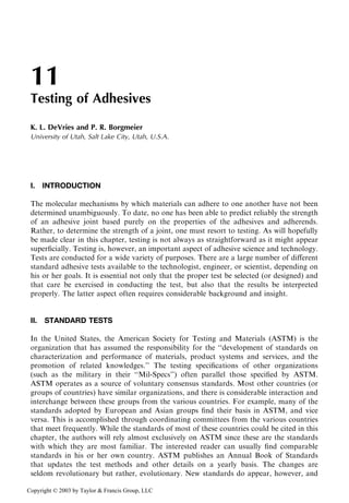
joint. The finger joints used to produce longer pieces of lumber or in other wood construction are a familiar example of such techniques. Figure 1 clearly demonstrates the
difference in bond area between a butt joint and one of the types of finger joint assemblies

Figure 1 Typical finger joint.

described in ASTM D-4688. It is noted that this geometry also results in a change in the
stress state. The butt joint appears to be dominated by tensile stresses (superficially at
least). Differences in elastic–viscous–plastic properties between the adhesive and adherends induce shear stresses along the bond line even for the case of the pure butt joint, but
the dominant ‘‘direct’’ stresses are tensile. (This is perhaps an opportune point to note
that, as explained in more detail later, the stress distribution in joints is almost never as
simple as it might first appear.) Clearly, for the tensile-loaded finger joint, shear stresses as
well as tensile stresses are applied directly to the bond line. Another reason why tensile
joints are avoided in design is because it has been observed empirically that many adhesives exhibit lower strength and high sensitivity to alignment when exposed to butt-type
tensile stresses.
However, a variety of standard tensile tests are available. Sample geometries for
some of the more common of these are shown schematically in Fig. 2. Figure 2a is a
schematic representation of the configuration from ASTM D-897. It is used (with slight
geometric alterations) for various adherends, ranging from wood to metal. It is often
called the, ‘‘pi tensile test’’ because the diameter is generally chosen to yield a crosssectional area of one square inch. Detailed specifications for U-shaped grips machined
to slip over the collar on the bonded spool-shaped specimen, to help maintain alignment
during loading, are given in the same standard. Our experience has been, however, that
even with such grips, reasonable care in sample manufacture, and acceptable testing
machine alignment, it is difficult to apply a really centric load. As a consequence, such
experiments often exhibit quite large data scatter [1,2]. The specimens for ASTM D-897
are relatively costly to manufacture. To reduce this cost, ASTM D-2094 specifies the use of
simpler bar and rod specimens for butt tensile testing. The D-2094 half specimens show in

Figure 2 Tensile adhesion test geometries: (a) pi tensile test, ASTM D-897; (b) bar and rod tensile
test, ASTM D-2094; (c) sandwich tensile test, ASTM D-257; (d) cross-lap tension test, ASTM
D-1344.

Fig. 2b are loaded by pins through the holes. The testing specification also describes a
fixture to assist in sample alignment, but this still remains a problem.
The specimens of both ASTM D-897 and D-2094 can be adapted for use with
materials that cannot readily be manufactured into conventional specimen shapes, by
the approach shown schematically in Fig. 2c. Such materials as plates of glass or ceramics
and thin polymer films can be sandwiched between the spool-like sections made of materials that can be more readily machined such as metals. Obviously, to obtain meaningful
results from this test, the strength of the adhesive bond to the spool segments must be
greater than that to the thin film or sheet.
ASTM D-1344 describes a cross-lap specimen of the type shown in Fig. 2d for
determining tensile properties of adhesive bonds. Wood, glass, sandwich, and honeycomb materials have been tested as samples in this general configuration. Even under
the best of circumstances, one would not anticipate the stress distribution in such a
case to be very uniform. The exact stress distribution is highly dependent on the
relative flexibilities of both the cross beams and the adhesive. Certainly, caution
must be exercised when comparing tensile strength from this test with data obtained
from other tensile tests. Probably for these reasons, this test is scheduled by ASTM for
discontinuation.
The results from these ‘‘tensile’’ tests are normally reported as the force at failure
divided by the cross-sectional area. Such average stress information can be misleading.
The importance of alignment has already been discussed. Even when alignment is ‘‘perfect’’ and the bonds are of uniform thickness over the complete bond area, the maximum
stresses in the bond line can differ markedly from the average stress [3,4]. The distribution
of stresses along the bond line is a strong function of the adhesive joint geometry. This is
demonstrated in Fig. 3, which shows both the normal and shear stress distribution as a
function of position for specimens of the general shape shown in Figs. 2a and b. These
calculations assume an elastic adhesive that is much less rigid than the steel adherends and
with a Poisson ratio of 0.49. The various curves in Fig. 3 represent differing diameter/
adhesive thickness ratios, shown as the parameters listed for each curve. Note that both
the normal stresses and the induced shear stress vary dramatically over the bonded surface. As described later, an understanding of stress and strain distribution in the adhesives
and adherends is useful in fracture mechanics analysis. The average stress results commonly reported from standard tensile tests must be used with great caution in attempts at
predicting the strength of different joints, even where the joints may be superficially
similar. References 2 and 4 use numerical and experimental techniques to explore the
effect of adhesive thickness on the strength of butt joints. The analysis and associated
experimental results in these references illustrate that the strength of the joint and the locus
of the point from which failure initiates are highly dependent on the adhesive thickness/
diameter ratio.
2. Shear Tests
Some of the most commonly used adhesive joint strength tests fall under the general
category of lap shear tests. Such samples are relatively easy to construct and closely
resemble the geometry of many practical joints. The stress distribution for lap joints is
far from uniform, but again the test results are commonly reported as load at failure
divided by the area of overlap. The maximum stress generally differs markedly from
this average value. More important, perhaps, failure of the joint is, in all likelihood,
more closely related to the value of the induced cleavage stresses at the bond termini

Figure 3
ratio.

Axial and shear stress distributions in butt joints, n ¼ 0.49. D/h is diameter/thickness

than to the shear stresses. Figure 4 shows several of the commonly used lap shear specimen
geometries (i.e., those corresponding to ASTM D-1002, D-3165, and D-3528).
Because of ﬂow of adhesive out the sides and edges as well as other diﬃculties in
preparing and aligning the parts when preparing individual lap specimens, samples are
frequently prepared from two relatively large sheets and the specimens are ‘‘saw’’ cut from
the resulting laminated sheet. This is illustrated in Figs. 4b and 5 and described in ASTM
D-3165. It has long been recognized that lap shear specimens such as those represented in

Figure 4 Standard lap shear geometries: (a) simple lap joint test, ASTM D-1002; (b) laminated lap
shear joint test, ASTM D-3165; (c) double lap joint test, ASTM D-3528.

Fig. 4a and b must distort, so that the forces applied to the sample fall on the same line of
action. This induces cleavage stresses in the adhesive near the bond termini. Double lap
shear specimens described in ASTM D-3528 are proposed as a means of alleviating this
problem (see Fig. 4c). However, based on our computer analysis and experimental studies,
we feel that failure of double lap joints is still dominated by cleavage stresses [5].
As was the case for tensile specimens, the stress distribution in lap joints is intricately
related to the details of the specimen geometry [2,6–16]. Such factors as amount of overlap, adhesive thickness, adherend thickness, relative stiﬀness (moduli) of the adhesive and
adherend, and other factors critically inﬂuence the stress distribution. The maximum

Figure 5 Large panel used to manufacture ASTM D-3165 specimens. The panel is cut into strips
for testing.

Figure 6 Log stress plot for the lap shear test.

stresses occur near the bond termini. Figure 6 shows the results of an elastic finite element
analysis for the stresses in this region for a specimen of ASTM D-1002 geometry. Note
that the tensile stresses are consistently higher than the shear. This fact, coupled with the
fact that adhesives have typically been shown to be more susceptible to cleavage than shear
failure, is consistent with the observation that cleavage rather than shear stresses usually
dominate lap joint fracture.
A reason that one should be very cautious in attempting to use average shear stress
criteria to predict failure of lap joints is illustrated in Fig. 7. This figure shows the force
required to cause failure in ASTM D-1002 lap joint specimens using steel adherends of
differing thicknesses. Note that for a given applied load, the ‘‘average shear stress’’ for all
adherend thickness would be the same (i.e., the applied force divided by the area of

Figure 7 Force required to cause failure versus adherend thickness for ASTM D-1002 specimens
using adherends of differing thicknesses.

overlap). If there was a one-to-one correspondence between this stress and failure, one
would expect failure load to be independent of the adherend thickness. It is obvious from
this figure that this is not the case. Similar results were obtained by Guess et al. [8]. The
trends shown in Fig. 7 can be quantitatively explained using numerical methods and
fracture mechanics [2,8]. Fracture mechanics is discussed later in the chapter.
A further indication of the popularity of lap shear tests is the number and variety of
such tests that have been standardized as illustrated in the following examples. ASTM:
D-905, Standard Test Method for Strength Properties of Adhesive Bonds in Shear by
Compression Loading, describes test geometry, a shearing tool, and procedures for testing
wood and similar materials. ASTM D-906, Standard Test Method for Strength Properties
of Adhesive in Plywood Type Construction in Shear by Tension Loading, provides specifications for specimen shape and dimensions, grips and jaws, and testing procedures for
testing plywood materials. ASTM D-2339 is a very similar test for plywood construction
materials. ASTM D-3930 describes several adhesive tests, including a block shear test for
wood-based home construction materials. D-3931 is similar to D-905, but for testing gapfilling adhesives; ASTM D-3163 and D-3l64 are similar to D-1002, except for use with
plastics and plastic to metal instead of metal to metal. ASTM D-3983, Standard Test
Method for Measuring Strength and Shear Modulus of Non Rigid Adhesives by a
Thick Adherend Tensile Lap Specimen, describes a dual-transducer slip gauge, specimen
geometry, and methods for determination of adhesive joint strength and modulus. ASTM
D-4027 has a similar purpose but uses a more complex ‘‘modified-rail test’’ apparatus.
ASTM D-4501 describes a shear tool and holding block arrangement for use in testing the
force required to remove a square block of material bonded to a larger plate. D-4501
describes a shear test in which the specimen is a block bonded to a larger plate. D-4562
describes a shear test in which the specimen is a pin bonded inside a collar. The test uses a
press to force the pin through the collar, which rests on a support cylinder. The test results
in this case are the force required to initiate failure divided by the bonded area between the
pin and collar. ASTM E-229 also uses a pin-in-collar type of specimen except that here
torsional loading causes the failure. D-4896, Standard Guide for Use of Adhesive-Bonded

Single Lap-Joint Specimen Test Results, is intended to give insight into the interpretation
of the results from all the lap shear tests. At other points in ASTM Vol. 15.06 and in this
chapter, reference is made to other standard tests that use ‘‘shear-type specimens’’ to
explore moisture, and other environmental, fatigue, and creep eﬀects in adhesive joints.
3. Peel Tests
Another common type of test is the peel test. Figure 8 shows four common types of peel
specimens. One can understand the test described in ASTM D-1876 by examining Fig. 8a.

Figure 8 Some standard peel test geometries: (a) T-peel test specimen, ASTM D-1876; (b) typical
testing jig used in ASTM D-1876; (c) climbing drum peel test, ASTM D-1781; (d) 180 peel test,
ASTM 903.
Copyright © 2003 by Taylor Francis Group, LLC

Figure 8 (Continued).

In this adhesive peel resistance test, often called the T-peel test, two thin 2024-T3 aluminum or other sheets typically 152 mm wide by 305 mm long are bonded over an area
152 mm wide by 229 mm long. The samples are then usually sheared or sawed into
strips 25 mm wide by 305 mm long (at times, the sample is tested as a single piece). The
76-mm-long unbonded regions are bent at right angles, as shown in Fig. 8a to act as tabs
for pulling with standard tensile testing grips in a tensile testing machine.
In a related test, one of the adhering sheets is either much stiffer than the other or is
firmly attached to a rigid support. Various jigs have been constructed to hold the stiffer
segment at a fixed angle to the horizontal and, by using rollers or other means, allow it to
‘‘float’’ so as to maintain the peel point at a relatively fixed location between the grips and
at a specific peel angle, as show schematically in Fig. 8b (see, e.g., ASTM D-3167).
ASTM D-1781 describes the climbing drum peel test that incorporates light, hollow
drums in spool form. The sample to be peeled is attached on one end to the central
(smaller) part of spool. The other end of the sample is affixed to the clamp attached to
the top of the crosshead of the tensile testing machine, as illustrated in Fig. 8c. Flexible
straps are wrapped around the larger-diameter part of the spool and attached to the other
crosshead of a loading machine. Upon loading, the flexible straps unwind from the drum
as the peel specimen is wound around it and the drum travels up (hence the name ‘‘climbing drum peel test’’), thereby peeling the adhesive from its substrate.
One of the simplest peel tests to conduct is the 180 peel test described in ASTM 903,
Standard Test Method for Peel or Stripping Strength of Adhesive Bonds. In this test, one
adherend is much more flexible than the other, so that upon gripping and pulling the two
unbonded ends, the sample assumes the configuration shown in Fig. 8d.

Clearly, peel strength is not an inherent fundamental property of an adhesive. The
value of the force required to initiate or sustain peel is not only a function of the adhesive
type but also depends on the particular test method, rate of loading, nature, thickness of
the adherend(s), and other factors [17]. Regardless, the peel test has proven to be a useful
test for a variety of purposes.
The authors have been impressed with the interesting studies at the University of
Akron [18,19], where Gent and his associates have used a peel test to measure the ‘‘work of
adhesion.’’ The work of adhesion is essentially synonymous with adhesive fracture energy,
discussed in Section III.C. Gary Hamed has published an article reviewing some of the
work at Akron [17]. This paper describes how peel tests have been used to, among other
things, (1) verify the usefulness of WLF time–temperature superposition, (2) investigate
dependence of the adhesive fracture energy on bond thickness, (3) study adherend thickness effects on adhesive strength, and (4) examine the effects of peel angle. J. R.
Huntsberger has also written an interesting discussion on the interpretation of peel test
results [20]. Others who have analyzed the stresses, energy dissipation, slip–stick phenomena, and other aspects of peel adhesion include Kaelble [21,22], Igarashi [23], Gardon [24],
Dahlquist [25], Bikerman [26], and Wake [27].
Another type of test, somewhat related to both tensile and peel, are the cleavage
tests, such as described in ASTM D-1062 and D-3807. This test uses a specimen that
resembles the compact tension specimen used for fracture of metals except that there is
an adhesive bond line down the sample center. The stresses for such a geometry are
nonuniform, but typical test results are given as force per width (i.e., failure-loaded divided
by bond width). ASTM D-3807 uses a specimen fabricated by bonding two narrow, long
rectangular beams together to form a split double cantilever beam. The force required to
initiate separation between the beams is measured and reported as average load per unit
width of beam. ASTM 3433, 3762, and 5041 also make use of cleavage specimens. These
are discussed in Section III.C because they are commonly used for determination of
adhesive fracture energy. D-1184, Standard Test Method for Flexure Strength of
Adhesive Bonded Laminated Assemblies, makes use of standard beam theory to calculate
the interlaminar shear strength in laminated beams loaded to failure.

B.

Environmental and Related Considerations

Adhesives are often used in applications where they are exposed to continuous or intermittent loads over long periods. It is difficult to duplicate such conditions in the laboratory. Neither is adhesive testing and/or observation under actual service conditions a very
feasible alternative. The designer is not usually able or willing to await the results of years
of testing before using the adhesive, and to tie up testing equipment and space for such
long periods would be prohibitively expensive. There are, however, companies, universities, and other industry groups that have loading racks or other test systems where samples
are exposed to dead weight or other loadings while exposed to ‘‘natural-weathering’’
conditions. It is advantageous, however, to have these backed up with (and an attempt
made to relate them to) accelerated tests. These accelerated tests are generally experiments
in which extreme conditions are used to increase the rate of degradation and deterioration
of the adhesive joint. Although it is seldom possible to establish a one-to-one correlation
between the rate of deterioration in the accelerated test and actual weather-aging conditions, it is hoped that the short-term tests will, at the very least, provide a relative ranking
of adhesive–adherend pairs, surface preparation, bonding conditions, and so on, and/or

provide some insight into relative expected lifetimes. As with all tests, the tester/designer
should use all of his or her knowledge, common sense, and insight in interpreting the data.
Some accelerated tests are surprisingly simple and intended to give only highly
qualitative information, while others have been formulated into standard tests intended
to yield more quantitative results. Since heat and moisture, to which adhesive joints are
commonly exposed, are environmental factors known to greatly influence adhesive durability, most accelerated tests involve these two agents.
As an example of a simple qualitative test we would like to cite a test devised by the
late E. Plueddemann of Dow Corning [28]. Plueddemann was perhaps the world’s foremost researcher in the area of silane coupling agents, bifunctional compounds with one
end of the molecule designed to react with oxygen or similar molecules on the substrate
(e.g., an oxide layer on a metal) and the other end designed to react with the polymer in the
adhesive [29–31]. In this way, a covalent ‘‘bridge’’ is developed between the adherend and
the adhesive. One of the main goals of these treatments is to reduce moisture deterioration
of the bond line. Accordingly, Plueddemann had need for a test to access quickly this
aspect of the wide variety of silanes produced and differing substrates. He devised the
following simple test for this purpose.
In his test, a thin film of adhesive on a glass microscope slide or a metal coupon is
cured and soaked in hot water until the film can be loosened with a razor blade. There is
usually a sharp transition between samples that exhibited cohesive failure in the polymer
and those which exhibited more of an interfacial failure. Since the diffusion of water into
the interface is very rapid in this test, the time to failure is dependent only on interfacial
properties and may differ dramatically between unmodified epoxy bonds and epoxy bonds
primed with an appropriate silane coupling agent. The time to debond in the hot water for
various silane primers differed by several thousandfold when used with a given epoxy. In
parallel tests, a thick film of epoxy adhesive on nonsilaned aluminum coupon showed
about the same degree of failure after 2 h in 70 C water as a silaned joint exhibited after
more than 150 days (3600 h) under the same conditions.
The authors have, several times, heard Plueddemann express the opinion that he
would be willing to guarantee that an adherend–silane–adhesive system that could withstand a few months of exposure to the conditions of his accelerated test would last many
decades under normal outside exposure conditions. He was quick to point out that this
guarantee does not cover other types of deteriorations of the adherends or adhesive (e.g.,
corrosion or polymer degradation) and that because of his age and health, he would not be
around to honor the guarantee. Nevertheless, he was very convinced (and convincing) that
his test was an ‘‘acid test’’ much more severe than most practical adhesive joints would
ever experience in their lifetime.
Perhaps, the best known test of this type is the Boeing wedge test, a form of which is
standardized in ASTM D-3762. Figure 9 shows this type of specimen and a typical plot of
results reported by McMillan, and his associates at Boeing [32,33]. Theidman et al. [34]
have also used the-wedge to investigate coupling agents.
Since adhesives have long been used in the wood/lumber business, where outdoor
exposure is inevitable, many of the standard accelerated tests were originally developed for
these materials. Such tests are increasingly finding uses for other materials. The most
common accelerated aging tests are:
1.

ASTM D-1101, Standard Test Method for Integrity of Glue Joints in Structural
Laminated Wood Products for Exterior Use. Two methods are outlined in this
standard for using an autoclave vessel to expose the joint alternately to water at


Figure 9 Boeing wedge test and typical results.

2.

3.

4.

vacuum pressure (ca. 635 mmHg) and low temperature with a high-pressure
stage (ca. 520 kPa), followed by a high-temperature drying stage (ca. 65 C circulated dry air). After the prescribed number of cycles (typically one or two), the
samples are visually inspected for signs of delamination.
ASTM D-1183, Standard Test Methods for Resistance of Adhesives to Cyclic
Laboratory Aging Conditions. This standard describes several different test
procedures in which the joints of interest are subjected to cycles made up of
stages at different relative humidities and temperatures, high-temperature drying
cycles, and/or immersed in water for specified periods. The joints are then evaluated by standard strength tests (lap joint, tensile, or other) to ascertain the
extent of degradation in strength.
ASTM D-2559, Specifications for Adhesives for Structural Laminated Wood
Products for Use Under Exterior (Wet Use) Exposure Conditions. Like
ASTM D-1101, this test makes use of an autoclave-vacuum chamber to impregnate specimens with water followed by drying in a hot (65 C) air-circulating
oven. A more quantitative measure of degradation is obtained in this test by
measuring lap shear compressive strength and measuring deformation as well as
visual evaluation to determine the extent of delamination.
ASTM D-3434, Standard Test Method for Multiple-Cycle Accelerated Aging
Test (Automatic Boil Test) for Exterior Wet Use Wood Adhesives. This standard describes the construction of apparatus to expose adhesive joints automatically to alternate boil/dry cycles. A typical cycle is composed of (a) submerging
the specimen for 10 min in boiling water, (b) drying for 4 min with 23 C air


5.

6.

circulating at 1.75 m/s, and (c) exposing the specimen for 57 min to 107 C air
circulating at 1.75 m/s. At a prescribed number of cycles, 10 specimens are withdrawn and their tensile shear strength measured and compared to tests on samples that have not been exposed to the accelerated testing conditions.
ASTM D-3632, Standard Practice for Accelerated Aging of Adhesive Joints by
the Oxygen-Pressure Method. This test is intended to explore degradation in
elastomer based and other adhesives that may be susceptible to oxygen degradation. The practice involves subjecting specimens to controlled aging environments for specified times and then measuring physical properties (shear or
tensile strength or other). The controlled environment consists of elevated temperature (70 C) and high-pressure (2 MPa) oxygen.
ASTM D-4502, Standard Test Method for Heat and Moisture Resistance of
Wood–Adhesive Joints. Rather than using an expensive autoclave as in D-1101
and D-2559, moisture aging in this test is accomplished in moist aging jars. The
samples are exposed to prescribed temperature–humidity cycles in the jars
heated in ovens. The strength of the aged samples is measured by standard
methods and compared to similar virgin samples.

There are tests that have been developed for use with solid polymer specimens that
find some use with adhesives. Ultraviolet (UV) radiation (e.g., as present in sunlight) is
known often to have detrimental effects on polymers. Accordingly, a popular accelerated
weathering (aging) test, ASTM G-53, ‘‘Standard Practice for Operating Light- and WaterExposure Apparatus (Fluorescent UV-Condensation Type) for Exposure of Nonmetallic
Materials,’’ describes use of a ‘‘weatherometer’’ that incorporates UV radiation moisture
and heat. These commercially available devices consist of a cabinet in which samples are
mounted on aluminum panels, which in turn are stacked edgewise on a sloped rack along
either side of the cabinet. These samples are then alternately exposed to two stages in
periodic cycles: a condensation stage followed by a UV-drying stage. The first stage is
accomplished by heating water in a partially covered tank below the specimens in the
bottom of the cabinet. The specimens are maintained at a constant temperature (typically
30 to 50 C) which is lower than the water temperature. This results in moisture condensation on the specimens. This stage might last for 1 to 4 h as selected by the operator. This is
followed by the UV-drying stage. An array of special fluorescent light tubes are situated
along each side of the cabinet parallel to the rack-mounted samples. The operator selects a
temperature higher than the condensation temperature (typically 40 to 70 C) that the
system automatically maintains in the cabinet for a fixed period (usually 1 to 40 h)
while the specimens are exposed to the UV radiation. The weatherometer is equipped
with a timer, a float-controlled water supply for the tank, and other controls, so that it
can continuously cycle through this two-stage cycle for months or even years with minimum operator care. Samples are removed periodically and their strength measured by
standard techniques for comparison with virgin samples and aged and virgin samples of
other materials. Many adherends are opaque to UV light, and hence one might question
the use of this weatherometer to explore weathering aging of adhesives used with such
adherends. However, even here, having such a commercial automated device might be very
useful. Both the condensation and radiation-heat curing stages are very analogous to
environmental exposures experienced by practical joints. This, along with the automated
and ‘‘standard’’ nature of the equipment, often makes the technique quite attractive.
More important, there are problems where the UV part of the aging may be critically
important. An example would be the bonding of a thin transparent cover film to a thin

sheet containing the reflective elements in sheeting used to make reflecting road signs. This
device would have obvious advantages in such cases and, indeed, has become the standard
for use in evaluating weather durability in that industry.
It is recognized that most accelerated tests do not duplicate or even closely approximate actual service conditions. As a case in point, most joints will, in all probability, never
be exposed to boiling water. It is hoped, however, that resistance to boiling for a few hours
or days may provide some valid evidence (or at least insight) into the durability of a
laminated part after years of exposure to high ambient humidity and temperature.
While such accelerated tests are never perfect, they may be the only alternative to observing a part in actual service for decades. The authors feel this philosophy is well stated in
Section 1.1 of ASTM D-1183: ‘‘It is recognized that no accelerated procedure for degrading materials correlates perfectly with actual service conditions, and that no single or small
group of laboratory test conditions will simulate all actual service conditions.
Consequently, care must be exercised in the interpretation and use of data obtained in
this test.’’ ASTM D-3434 includes the following statement about its significance: ‘‘The test
method assumes that boil/dry cycling is an adequate and useful accelerated aging technique.’’ Evaluation of long-term durability of adhesives in wood joints under severe service
conditions, including extended exterior exposure, is a complex field, and no entirely reliable short-term test is known to ensure that a new type of adhesive system will resist
satisfactorily all of the chemical, moisture, microorganism, and solvent effects that such
severe service may involve. Except for the effects of microorganisms and similar biological
influences, this test method has proven very useful for comparison purposes to distinguish
between adhesive systems of different degrees of durability to the usual temperature,
moisture, and cyclic moisture conditions. It has proven very useful to distinguish between
bond lines, made with adhesives of proven chemical and biological durability, that when
properly used in production resist the mechanical and moisture effects that such joints
must withstand in severe service over extended periods of exposure. It does not, however,
in itself, assure that new types of adhesives will always withstand actual exterior or other
severe service.
Other environmental related tests include ASTM D-904, Standard Practice for
Exposure of Adhesive Specimens to Artificial (Carbon-Arc Type) and Natural Light;
ASTM D-1828, Standard Practice for Atmospheric Exposure of Adhesive-Bonded
Joints and Structures; ASTM D-1879, Standard Practice for Exposure of Adhesive
Specimens to High Energy Radiation; and ASTM D-3310, Standard Test Methods for
Determining Corrosivity of Adhesive Materials.
In practical joints, adhesives are not always loaded statically or loaded for short
periods of time. To help evaluate the performance of stressed adhesive joints as a function
of time, tests have been developed to determine the response of adhesive joints to creep
and cyclic loading. ASTM D-1780, Standard Practice for Conducting Creep Tests of
Metal-to-Metal Adhesives, makes use of a deadload weight-lever loading frame to measure creep of lap shear specimens. ASTM D-2793, Standard Test Method for Creep of
Adhesives in Shear by Compression Loading (Metal-to-Metal), describes the constructions and procedures for use of creep test apparatus in which the sustained loading is
maintained by springs. ASTM D-2294 is similar to D-2293, except that here the springloaded apparatus loads the lap specimen in tension. ASTM D-4680, Standard Test
Method for Creep and Time to Failure of Adhesives in Static Shear by Compression
Loading (Wood-to-Wood), describes the construction of a spring-loaded apparatus and
testing procedures for a creep apparatus for use with relatively large wood specimens.
ASTM D-2918 and D-2919 describe tests to measure the durability of adhesive joints in

peel and lap shear, respectively. The tests and recommended fixtures are intended to hold
specimens under sustained loadings while exposed to environments such as moisture, air,
vapors, water, or other environments.
ASTM D-3166, Standard Test Method for Fatigue Properties of Adhesives in Shear
by Tension Loading (Metal-to-Metal), provides procedures for testing and measurement
of the fatigue strength of lap specimens. It makes use of conventional tensile testing
machines capable of applying cyclic axial loads. Researchers have also made beneficial
use of the concepts of fracture mechanics to evaluate the fatigue crack growth rate per
cycle, da/dn, as a function of stress intensity factor. For this purpose, Mostovoy and
Ripling [35], for example, have used fracture mechanics specimens similar to those
described in ASTM D-3433. Fracture mechanics is discussed at the end of this chapter
as well as in many books.
Adhesive joints are frequently exposed to sudden dynamics loads, and hence a
knowledge of how adhesives react to impact loading is important for some applications.
ASTM D-950, Impact Strength of Adhesive Bonds, describes sample configuration and
testing apparatus for measuring the impact strength of adhesive bonds. The method is
generally analogous to the Izod test method used for impact studies on a single material.
ASTM D-2295 describes apparatus that utilizes tubular quartz lamps to investigate
failure of adhesive joint samples at high temperatures, and ASTM D-2257 outlines procedures for testing samples at low temperatures (À 268 to À 55 C). ASTM also provides
specific standards to investigate failure-related properties of adhesives that are less directly
related to mechanical strength. Such properties include resistance to growth and attack by
bacteria, fungi, mold, or yeast (D-4300 and D-4783), chewing by rodents (D-1383), eating
by insects (D-1382), resistance to chemical reagents (D-896), and so on. It is enough to
make the adhesive designer or researcher paranoid. Not only are stresses, temperatures,
moisture, and age working against him or her, but now it appears that microorganisms
and the animal kingdom want to take their toll on any adhesively bonded structure.
Although the primary purpose of this chapter is to discuss mechanical testing and
strength of adhesive joints, the reader should be aware that ASTM covers a wide variety of
tests to measure other properties. ASTM, for example, includes standard tests to measure
the viscosity of uncured adhesives, density of liquid adhesive components, nonvolatile
content of adhesives, filler content, extent of water absorption, stress cracking of plastics
by liquid adhesives, odor, heat stability of hot-melt adhesives, ash content, and similar
properties or features of adhesives.
Of particular interest to the adhesive technologist are surface treatments. ASTM has
adopted standard practices for treating surfaces to better adhesives. ASTM D-2093,
Standard Practice for Preparation of Plastics Prior to Adhesive Bonding, describes physical
chemical, and cleaning treatments for use on a wide variety of polymer adherends. D-2651,
Standard Practice for Preparation of Metal Surfaces for Adhesive Bonding, describes techniques, cleaning solutions and methods, etchants or other chemical treatment, and so on,
for metal adherends, including aluminum alloys, steel, stainless steel, titanium alloys,
copper alloys, and magnesium alloys. ASTM D-2675 is concerned with the analysis and
control of etchant effectiveness for aluminum alloys. ASTM D-3933 provides a standard
practice for phosphoric acid anodizing of aluminum surfaces to enhance adhesion.
C. Fracture Mechanics Techniques
As noted earlier, the most commonly used standards for determination of adhesive joint
properties and characteristics suggest reporting the results in terms, of average stress at

failure. If average stress criteria were generally valid, one would anticipate that a doubling
of the bond area should result in a proportionate increase in joint strength. Studies in our
laboratory demonstrate that such criteria may lead to erroneous predictions [36]. This
study involved leaving half of the overlap area unbonded. All of the samples had the same
amount of overlap. Part of the samples (the control) were bonded over the complete
overlap region. Part of the overlap area near one of the bond termini was without any
adhesive and the other part had a 50% unbonded region centered in the overlap region. In
neither case was the reduction in strength commensurate with the reduction in bond area.
That is, for the end debonds, the reduction in load at failure averaged less than 25% and
for the center debonds it was reduced by less than 10%. This is consistent with standards
such as ASTM D-3165, Strength Properties of Adhesives in Shear by Tension Loading of
Laminated Assemblies, which address the fact that average lap shear strength is dependent
on different bond areas of the joint and that the adhesive can respond differently to small
bond areas compared to large bond areas.
To determine failure loads for different geometries, other methods are required. This
is due to the fact that the stress state in the bond region is complex and cannot be
approximated by the average shear stress. A method that is gaining in popularity for
addressing this problem is the use of fracture mechanics. With the use of modern computers, the stress state and displacement even in complex adhesive bonds can be determined
with good accuracy. A fracture mechanic approach uses these stresses combined with the
displacements and strains and conservation of energy principles to predict failure conditions. At least three ASTM standards are based on fracture mechanics concepts (ASTM
D-3433, D-3762, and D-5041). The premise behind fracture mechanics is accounting for
changes in energies associated with the applied load, the test sample, and the creation of
new surface or area. Since fracture mechanics techniques are well documented in the
literature (see, e.g., Refs. 37 and 38), only a brief review is presented here.
The methods suggested here are formulated using methods similar to those postulated
by Griffith [39]. Griffith hypothesized that all real ‘‘elastic’’ bodies have inherent cracks in
them. He hypothesized that a quantity of energy to make the most critical of these cracks
grow would need to come from the strain energy in the body and work applied by
loads. Conservation of energy dictates that a crack can grow only when the strain energy
released as the crack grows is sufficient to account for the energy required to create the new
‘‘fracture’’ surface. In Griffith’s original work, he considered only perfectly elastic systems.
He conducted his confirmation experiments on glass, which behaves as a nearly ideal elastic
material. In this case the fracture energy is very closely associated with the chemical surface
energy. Indeed, Griffith was able to establish such a correlation by measuring the surface
tension of glass melts and extrapolating back to room temperature. Most engineering solids
are not purely elastic and the energy required to make a crack grow involves much more
than just the chemical surface energy. In fact, the energy dissipated by other means often
dominates the process and may be several orders of magnitude higher than the chemical
surface energy term. As explained in modern texts on fracture mechanics, this has not
prevented the use of fracture mechanics for analysis of fracture in other quasi-elastic systems, where typically the other dissipation mechanisms are lumped into the fracture energy
term Gc (discussed later). Techniques are also being developed to use the basic approach for
systems that experience extensive viscoelastic and plastic deformation. These approaches
are more complex. Here we confine our attention to quasi-elastic cases. Significant research
and development work has gone into methods of increasing the dissipative processes
required for a crack to grow, thereby, ‘‘toughening’’ the materials. As a consequence,
another name for the fracture energy is fracture toughness Gc.

While Griffith’s earlier fracture mechanics work was for cohesive fracture, the
extension to adhesive systems is logical and straightforward. In the latter case, one must
account for the strain energy in the various parts of the system, including adherends and
adhesive, as well as recognizing that failure can proceed through the adhesive, the
adherend, or the interphase region between them. Here too, energy methods can be
useful in determining where the crack might grow since one might anticipate that it
would use the path requiring the least energy.
In principle, the fracture mechanics approach is straightforward. First, one makes a
stress-strain analysis, including calculation of the strain energy for the system with the
assumed initial crack and the applied loads. Next, one performs an energy balance as the
crack proceeds to grow in size. If the energy released from the stress field plus the work of
external forces is equal to that required to create the new surface, the crack grows. A
difficulty in performing these analyses is that for many practical systems, the stress state is
very complex and often not amenable to analytical solutions. With the use of modern
computers and computational codes, this is becoming progressively less of a problem.
Finite element codes are refined to the point that very accurate stress–strain results can
be obtained, even for very complex geometries (such as adhesive joints). Furthermore, it is
possible to incorporate complex material behavior into the codes. The latter capability has
not reached its full potential to date, at least in part, because the large strain deformation
properties of the materials involved, at the crack tip, are not well defined.
A relatively simple example may help in understanding the application of fracture
mechanics. First, let’s assume that we have two beams bonded together over part of their
length, as shown in Fig. 10a. Here we will make two additional convenient (but not
essential) assumptions: (1) the adhesive bond line is sufficiently thin that when bonded
as shown in Fig. 10b, the energy stored in the adhesive is negligible compared to that in the
unbonded length of the beams a; and (2) the length a is sufficiently long that when loaded,
the energy due to bending dominates (i.e., the shear energy and other energy stored in the
part of the beam to the right of a is negligible).

Figure 10

Double cantilever beam specimen showing nomenclature and specimen deflection.


The end deflection of the unbonded segment of each beam due to a load P is found in
mechanics of material texts to be [40]
d¼

Pa3
3EI

ð1Þ

where a is the unbonded length, E the modulus of elasticity for the material from which the
beams are manufactured, and I the moment of inertia for a rectangular cross-section. The
work done by the forces P in deforming this double cantilever is therefore
1
W ¼ Pð2dÞ
2

ð2Þ

which for a conservative elastic system equals the energy U, where
U ¼ Pd ¼

P2 a3
3EI

ð3Þ

If we assume Griffith-type fracture behavior, the energy released as the crack grows
(a increases) must go into the formation of new fracture surface. The fracture energy Gc
(sometimes called energy release rate) is therefore
ÁU
ÁA
Substituting Eq. (3) into (4) and taking the limit leads to
Gc ¼

Gc ¼

@U 1 @U P2 a2 12P2 a2
¼
¼
¼
EIb
@A b @a
Eh3 b2

ð4Þ

ð5Þ

where
@A % 2aðbÞ

ð6Þ

We thus see that such beam systems could be used to determine Gc. Indeed, ASTM D-3433
makes use of such beams for this measurement. It should be noted that the equation given
in Section 11.1.1 of D-3433 has a similar form:
Gc ¼

4P2 ð3a2 þ h2 Þ
Eb2 h3

ð7Þ

This equation can be used for smaller values of a since it includes effects of shear and other
factors that, as noted above, were neglected in our simple analysis. Inspection of Eq. (7)
shows that as a becomes large compared to h, this equation reduces to that derived above.
By tapering the beams, ASTM shows how a related geometry can be used for Gc determination where the data analysis is independent of the crack length. The advantage here is
that one need not monitor crack length. An advantage of double cantilever beam specimens is that measurement can be made for several different values of a for a given beam,
making it possible to get several data points from a single sample. Conversely, if Gc is
known, say from another test configuration, fracture mechanics can be used to determine
the load required to initiate fracture.
The case described above is the exception rather than the rule. Most practical problems do not have stress and displacement fields easily obtained by analytical methods.
Numerical methods can be applied to obtain the necessary stress and displacements
needed to calculate the energy release rates. The basic consideration for calculating
energy release rates is accounting for the difference in energy before and after crack
extension dA. This condition can be approximated for a discrete system by using finite

element methods (FEMs), that is, by using a computer to calculate the strain energy
change as a crack area is incrementally increased.
Two different methods of calculating the energy release rate numerically are outlined
briefly. The first, the compliance method, is readily applied using FEM [37]. This method
requires only two computer runs for each energy release rate desired. The first computer
run is used to calculate the total relative displacement, ua, of the sample for the crack
length a, under a constant force F a. In the second computer run, a finite element node is
released, extending the crack to a length of a þ Áa. The second run allows calculation of
the total relative displacement, uaþÁa, of the sample for a crack length a þ Áa under the
same constant load F a. Using the discrete form of the energy release rate for a linear
elastic body leads to
G¼

F a ðuaþÁa À ua Þ
2ÁA

ð8Þ

The discrete form of the energy release rate under constant displacement assumptions for
the same crack length can easily be shown to be

1 À ua
a a
F u
u a þ Áa
G¼
ð9Þ
2ÁA
A third computer run can be used to extend the crack by releasing the next node in front of
the crack tip. This increases the crack length to a þ 2Áa. Letting uaþÁa equal the new
relative displacement and ua equal the total relative displacement from run 2, the energy
release rate for the new crack length can be computed using Eq. (8) or (9) with the addition
of only one computer run. This process can be repeated, each time determining a new
energy release rate per single computer run, thereby producing a curve of energy release
rate versus crack length. The crack length for which the energy release rate is equal to Gc is
a critical crack length where failure should ensue.
A second method for calculating energy release rate is the crack closure integral
(CCI) method [37,41–43]. This method uses FEM techniques to calculate the energy that
is needed to close a crack extension. It is assumed that for an elastic system this energy is
equivalent to the energy that is needed to create the crack’s new surface, giving an alternative method of calculating the energy release rate from that just discussed.
The CCI method is also readily accomplished using FEM. The energy release rate
calculated as outlined in the following is for a constant stress crack extension assumption.
In general, this method requires four computer runs for each energy release rate calculated. The method can be shortened to three computer runs if verifying that the crack was
closed is not necessary. In this case, only the second, third, and fourth steps explained
below need to be performed.
The first computer run is used to calculate the displacements (or locations) of the
finite element nodes near the crack tip for crack length a under constant load F a. Let uBX1
and uBY1 represent the displacements of the first bottom node in the X and Y directions,
respectively, from run 1. Let uTX1 and uTY1 represent the displacements of the first top
node in the X and Y directions, respectively, from run 1. Since we have not yet released this
first node for run 1, the top and bottom nodes are coincidental and should have the same
displacement. This initial displacement indicates the point to which the nodes will have to
be moved when the crack is closed in runs 3 and 4.
In the second computer run, a node is released extending the crack length to a length
of a þ Áa. This allows calculation of the new nodal positions of the same nodes that were

Figure 11
rates.

Pictorial of the ﬁrst and second steps in the CCI method of determining energy release

released from run 1 while under the constant load F a. Let uBX2 and uBY2 represent the
displacements of the bottom node in the X and Y directions, respectively, from run 2. Let
uTX2 and uTY2 represent the displacements of the top node in the X and Y directions,
respectively, from run 2. The distance between the top node and bottom node in the X and
Y directions indicates how far the nodes will need to be moved in each direction to close
the crack. Figure 11 shows computer runs 1 and 2 in a pictorial schematic and summary
of the two steps.
In the third run, vertical unit forces are applied to the released nodes in the direction
needed to bring them back to their original vertical positions. The nodal displacements of
these released nodes of the sample for a crack length of a þ Áa under the same constant
load F a are noted. Let uBY3 represent the displacement of the bottom node in the
Y direction from run 3. Let uTY3 represent the displacements of the top node in the
Y direction from run 3. The diﬀerence between the node displacements from runs 2 and
3 indicates how far the vertical unit force moved each node toward its original position.
The fourth run is the same as run 3 except that the forces are now horizontal.
Figure 12 shows computer runs 3 and 4 in a pictorial schematic and a summary of the
two steps.

Figure 12 Pictorial of the third and fourth steps in the CCI method of determining energy
release rates.

Runs 3 and 4 provide a measure of how much each node is moved back toward each
original position by unit forces. Since the material is modeled as linear elastic, the force
required to move each node back to its original position can be determined simply by
increasing these forces in proportion to the total displacements required to bring the nodes
back to their original position. We will call these forces FX and FY. The energies EX and EY
required to close the crack in the X and Y directions can now be calculated by determining
the work of these forces on the crack closure displacements since for an elastic system, the
work is stored as strain energy.
Based on this analysis, the energy release rates can be partitioned into the energy
release rates associated with crack opening displacement (GI) and shear displacement
normal to the crack surface (GII):
GI ¼
GII ¼

X
X
ÁE1 À ÁE2
ÁA
Y
Y
ÁE1 À ÁE2
ÁA


ð10Þ

The total energy release rate can be determined from
G ¼ GI þ GII

ð11Þ

In Eqs. (10) and (11), G represents the total energy release rate under constant-stress crack
extension assumptions, GI represents the portion of G in the mode I direction, and GII
represents the portion of G in the mode II direction. A couple of concluding comments to
this section might be in order. Each of these methods of solving for the fracture energy has
advantages. The compliance method is simpler and less expensive to perform. The crack
closure method, on the other hand, facilitates calculation of crack growth analysis under
different loading (i.e., crack opening or shear). There is evidence that cracks in materials
behave differently under the various loadings. As a consequence, growth of a given crack
may depend on the relative amounts of mode I and mode II stresses at its tip. It is also
advantageous to have the two methods of determining G. Since they provide a systematic
check on each other, that might be used to verify for code, programming, or other errors.
Computer-based energy release rates might be a very useful design tool. An example
might be used to illustrate such use. Assume that nondestructive evaluation techniques are
used to locate and determine the size and shape of a debond region in the interphase region
of an adhesive bond in a structure. An example of such a bond might be between a rocket
motor case and a solid propellant grain. A reasonable question would be: Is this ‘‘flawed’’
region ‘‘critical’’ in that it might cause failure under prescribed service load conditions?
For many structures (e.g., the rocket case noted) this might literally be a million dollar
question. A reliable answer could mean the difference between safely using the structure or
needing to repair or discard it. Trying to answer the question experimentally would generally be very expensive. An alternative approach might make use of fracture mechanics.
One might use FEM to model the structure, including the debond region that has been
identified. Using the techniques outlined above, the energy release rate can be calculated
for assumed increases in the size of debond. If the critical fracture toughness (Gc) is known
(perhaps determined from independent tests with standard specimens), it can be compared
with the value calculated. If the energy release rate calculated for the debond in the
structure is equal to Gc, the debond is apt to grow. If it is larger than Gc, the crack
should accelerate. Values of energy release rate significantly lower than Gc would indicate
a noncritical region. Other types of irregularities, cohesive or adhesive, might be treated in
a similar manner. Obviously, such an approach requires not only adequate FEM techniques and computers but also nondestructive means to identify and quantitatively measure
potential critical regions.
As a final note in this section, a few examples taken from the research of the authors
and their associates, on the utility of fracture mechanics in conjunction with numerical
analysis, might be informative. Some of the research in the authors’ laboratory has centered on identifying the loci of failure ‘‘initiation’’ and the paths followed by cracks as they
proceed through the adhesive in a joint.
Several rather different geometries have been investigated, some that were patterned
after standared test configurations and one designed to simulate a specific application. The
latter was a cone pull-out (or twist-out) specimen devised to simulate such dental adhesive
applications as fillings, caps, and crowns [42,44]. In this test configuration material in the
form of a truncated cone was bonded into a matching hole in a plate. Pulling (or twisting)
could initiate failure of the cone while the plate was held fixed. If the cone had a zero
degree cone angle, the test became a cylinder pull-out test. For the tests of interest here, the
cone and the plate were fabricated from transparent poly(methyl methacrylate) (PMMA)
and the adhesive was transparent polyurethane (Thiokol Solithane-113). The use of these

materials allowed visual observation of the bond line of the adhesive joint. The lower
1.6 mm (at the truncated cone end) was left unbonded to act as a starter crack. Finite
element analysis of this specimen, under stress, indicated that as the tip of this region was
approached the stresses induced in the adhesive became very large (singular). Somewhat
removed from this point, the stresses were finite and well behaved, independent of cone
angle.
When samples with a zero degree cone angle were pulled to failure, it was always
observed that the failure propagated from this starter crack. On the other hand, when the
cone angle was increased slightly (e.g., to 5 ), the initial failure was never observed to
originate at this starter crack. Rather, the first signs of failure were observed further up in
the joint—approximately halfway between the end of the starter crack and the other end
of the bond line. This crack then grew from that point until ultimate separation occurred.
The obvious question was, why did failure not occur at the point of ‘‘maximum stress,’’
i.e., at the starter crack? The numerical analysis did indicate that there was a local maximum in the stress at the point where failure was first observed but the value of this
maximum was significantly lower than that close to the singularity point. We feel the
answer lies in the difference in the nature of the energy release rate (ERR or G) at the
two points. A small (25 mm) ‘‘inherent’’ cracklike flaw was assumed to exist at the local
‘‘stress maximum’’ referred to above. The ERR was calculated for a crack proceeding
from this point and compared with the value of the ERR for a crack emanating from the
much larger starter crack. Even for such a small assumed inherent crack, the calculated
ERR was larger at the point halfway up on the specimen. The conclusion was that failure
is governed by the ERR and that failure initiation is at points of maximum ERR.
This same conclusion was substantiated by a series of tensile tests in which a butt
tensile joint specimen was formed by adhesively bonding a PMMA rod to a PMMA plate
with the polyurethane referred to above [42,44]. The specimens were set up in an Instron
testing machine adapted with holes and a mirror arrangement that allowed the bond line
to be observed and recorded with a video recorder. Finite element analysis indicated that
for small assumed cracklike flaws, the values of the ERR and the location of maximum
ERR were very strong functions of the ratio of the adhesive thickness to the joint diameter. As a consequence, the load required to propagate a crack should be a function of
the thickness of polyurethane, even for constant size initial cracks. Furthermore, since the
location of maximum ERR varied with this same thickness, one would anticipate the
location of crack growth initiation to vary. Experimentally, both features were observed:
(1) Variation in the value of the load required to propagate a crack was completely
consistent with the calculated variation in ERR with thickness. (2) When the ERR for
the assumed 25 mm inherent flaw was largest at the edge, cracks tended to start at the edge.
When the ERR was greater in the center, that was the location from which the crack was
observed to emanate. It is noted that, as with the cone test, finite element analysis indicated that the stresses at the bond line become singular as the outer diameter of the
specimen is approached (e.g., as r ! R0).
The final example involves fracture mechanics–finite element analysis of the double
cantilever beam (nontapered) specimen (see Fig. 10 as well as the figures and descriptions
in ASTM D-3433). The finite element analysis was very much as outlined above, leading to
Eqs. (8) through (11). These results were compared with the equations in Section 11.1.1 of
D-3433 (Eq. (7) in this chapter). Except for the longest cracks (i.e., very large a in Fig. 10),
the FEM-determined ERR differed appreciably from the Gc value determined from Eq.
(7). These differences might be attributed to the fact that the derivation of Eq. (7), similar
to that for Eq. (5), assumes ideal cantilever boundary conditions at the point x ¼ a.

Figure 13 Comparison of the ERR determined by FEM with G values calculated using the
equations from ASTM D-3433 as a function of the ratio of crack length, a, to couble Cantilever
beam specimen depth, h.

The assumed conditions are that there is no deﬂection and zero slope (i.e., no rotation) at
that point. Figure 13 (taken from [45]) illustrates that the diﬀerences in G, determined by
the two methods, might be 50% or more for small values of a. The experiments described
in ref. [45] demonstrate that much more consistent values of Gc are obtained when using
the FEM to calculate Gc, from the experimental results over typical a/h values, than when
they are calculated using the equation from D-3433. In the FEM case, the variation was
typically less than Æ 5%, while the variation using Eq. (7) could be ten times larger.
In addition to ignoring the energy associated with the nonideal cantilever conditions
just described, the derivation of Eqs. (5) and (7) also neglects any energy stored in the
adhesive. While this latter assumption might be valid for extremely thin adhesives, it is
noted that for many adhesive–substrate combinations the modulus of the adhesive is only
a few percent that of the adherends. As a result, for adhesives with thicknesses that are
5%, or so, of the adherend’s thickness the contribution of the strain energy in the adhesive
to the ERR (Gc) can be appreciable. This is also consistent with the experimental observations reported in ref. [44]. Inclusion of the strain energy in the adhesive in the total energy
balance facilitated an additional calculation/observation. Adhesive engineers and scientists
have long speculated on reasons for the common observation that cracks in adhesive joint
generally follow paths somewhat removed from the so-called adhesive–adherend
‘‘interface’’ rather than along this bond line. It might reasonably be assumed that
cracks would follow paths of maximum energy release rate, since this would be the path
where the most energy would be dissipated. In the FEM analysis, various crack paths were
assumed through the adhesive and the ERR determined [45]. By varying the adhesive and
adherend(s) thicknesses, it was possible to design double cantilever beam specimens in
which the path of Max-ERR was near the center of the adhesive, near one or other of the

Figure 14 Photographs showing the loci of crack growth for diﬀerent double cantilever beam
adhesive joint specimens pulled to failure. (a) The ERR calculated by FEM for this specimen was
largest down the center of the adhesive, (b) the ERR calculated by FEM for this specimen was
largest near the lower edge of the adhesive, and (c) the ERR calculated by FEM for this specimen
was essentially independent of position across the adhesive thickness.

edges of the adhesive, or relatively constant across the thickness. Samples of these differing
geometries were constructed of aluminum and an adhesive (both of which exhibited relatively linear elastic behavior) to simulate the linear elastic finite element calculations.
Starter cracks were introduced at different locations through the adhesive thickness.
These samples were pulled to failure, the fracture load recorded, and the locus of the
fracture path observed/noted. In every case, the experimentally observed fracture paths
closely followed the planes of Max-ERR determined by the finite element analyses. If the
starter crack was somewhat removed from this location, the ‘‘running’’ crack quickly
moved to the path of Max-ERR. Figure 14 [45] shows photographs of some samples
from these experiments. Photograph (a) was for a sample in which the FEM-determined
ERR was maximum at the center and the starter crack was at the edge. The crack started
at the starter crack and then moved to and ran nearly planar along the center. Photograph
(b) is for a sample with different thicknesses of adherends. Here the FEM-determined
ERR was at the lower edge of the adhesive and the starter crack was introduced at the
upper edge. The crack started at the starter crack but again quickly moved to and ran
along the path of Max-ERR. In (c) the FEM-determined ERR was relatively insensitive to
the exact path in the adhesive. Here, there was no ‘‘mechanical’’ reason for a preference
for a specific path and the crack wandered as apparently chemical or physical differences
in the adhesive dictated the exact path followed.
These analyses and associated experiments demonstrate that fracture mechanics can
be used to provide information and insight into the value of the failure load, the locus of
likely crack growth, and the path along which the crack will then grow. Where analytical
analyses of stress, strain, and energy release rates are difficult or impossible, modern
numerical methods can be very useful. In the opinion of the authors, the utility of these
combined tools has hardly been exploited. The inclusion of nonlinear, nonelastic effects in
the analyses is feasible is such materials are carefully characterized and/or properties
become available.

IV.

CONCLUSIONS

There are a great many properties that affect adhesive quality. One of the more important is
the strength of joints formed with the adhesive and adherends. We have discussed a number
of standard tests commonly used to ‘‘measure’’ adhesive joint strength. These methods are
valuable and serve many purposes. In this chapter, however, we point out that the use of the
‘‘standard’’ results from these tests to predict the strength of other joints that differ in even
seemingly minor details is questionable. A more reliable comparison between adhesives and
joints might be to compare more fundamental properties, such as moduli, adhesive fracture
toughness, and so on. This is a basic premise of fracture mechanics. With improved computation facilities and codes, these methods show promise for using results from standard
tests to predict the performance of other (perhaps more complex) practical adhesive joints.
As such, they should become very powerful design tools.

REFERENCES
1.

G. P. Anderson, S. Chandapeta, and K. L. DeVries, in Adhesively Bonded Joints: Testing,
Analysis, and Design, ASTM STP-981 (W. S. Johnson, ed.), American Society for Testing
and Materials, Philadelphia, 1988.


2. G. P. Anderson and K. L. DeVries, in Adhesion and Adhesives, Vol. 6 (R. Patrick, K. L. DeVries,
and G. P. Anderson, eds.), Marcel Dekker, New York, 1988.
3. G. P. Anderson, K. L. DeVries, and G. Sharon, in Delamination and Debonding of Materials,
ASTMP STP-876 (W. S. Johnson, ed.), American Society for Testing and Materials,
Philadelphia, 1985.
4. K. C. Grammol, M. S. thesis, Mechanical Engineering Department, University of Utah, 1984.
5. J. K. Strozier, K. J. Ninow, K. L. DeVries, and G. P. Anderson, in Adhesion Science Review
(H. F. Brinson, J. P. Wightman, and T. C. Ward, eds.), Commonwealth Press, Radford, VA,
1987, p. 125.
6. O. Volkersen, Luftfahrt Forsch. 15: 41 (1938).
7. M. Goland and E. Reissner, J. Appl. Mech. 11: 17 (1944).
8. T. R. Guess, R. E. Allred, and F. P. Gerstle, J. Testing Eval. 5(2): 84 (1977).
9. A. J. Kinloch, Adhesion and Adhesives Science and Technology, Chapman Hall, New York,
1987.
10. G. R. Wolley and D. R. Carver, J. Aircr. 8(19): 817 (1971).
11. R. D. Adams and N. A. Peppiatt, J. Strain Anal. 9(3): 185 (1974).
12. S. Amijima, A. Yoshida, and T. Fujii, in Proc. 2nd International Conference on Composite
Materials, Toronto, Ontario, Canada, Metallurgical Society of AIME, New York, 1978.
13. J. K. Sen and R. M. Jones, AIAA J. 18(10): 1237 (1980).
14. J. K. Sen and R. M. Jones, AIAA J. 18(11): 1376 (1980).
15. W. N. Sharpe and T. J. Muha, in Proc. Army Symposium on Solid Mechanics, AMMRC-MS75-8, Army Materials and Mechanics Research Center, Watertown, Mass., 1974, p. 23.
16. J. L. Hart-Smith, Douglas Aircraft Report 6922, Long Beach, California, 1980.
17. G. R. Hamed, in Adhesion and Adhesives, Vol. 6 (R. L. Patrick, K. L. DeVries, and
G. P. Anderson, eds.), Marcel Dekker, New York, 1988.
18. A. N. Gent and G. R. Hamed, J. Appl. Polymer Sci. 21: 2817 (1977).
19. A. N. Gent and G. R. Hamed, Polymer Eng. Sci. 17: 462 (1977).
20. J. R. Huntsberger, in Adhesion and Adhesives, Vol. 6 (R. L. Patrick, K. L. DeVries, and
21. D. H. Kaelble, Physical Chemistry of Adhesion, Wiley-Interscience, New York, 1971.
22. D. H. Kaelble and C. L. Ho, Trans. Soc. Rheol. 18: 219 (1974).
23. T. Igarashi, in Adhesive Joints, Formation, Characteristics and Testing (K. L. Mittal, ed.),
Plenum Press, New York, 1984.
24. J. L. Gardon, J. Appl. Polymer Sci. 7: 643 (1963).
25. C. A. Dahlquist, in Treatise on Adhesion and Adhesives, Vol. 2 (R. L. Patrick, ed.), Marcel
Dekker, New York, 1969.
26. J. J. Bikerman, The Science of Adhesive Joints, Academic Press, New York, 1968.
27. W. C. Wake, Adhesion and the Formulation of Adhesives, Applied Science Publishers, London,
1982.
28. E. P. Plueddemann, J. Adhesion Sci. Technol. 2: 179 (1988).
29. E. P. Plueddemann, Silane Coupling Agents, Plenum Press, New York, 1982.
30. F. J. Boerio, in Adhesion and Adhesives, Vol. 6 (R. L. Patrick, K. L. DeVries, and
31. S. Naviroj, J. L. Koenig, and H. Ishida, J. Adhesion 18: 93 (1985).
32. J. C. McMillan, in Bonded Joints and Preparation for Bonding: AGARD Lecture Series 102,
Technical Editing and Reproduction, London, 1979, Chap. 7.
33. J. C. McMillan, Developments in Adhesives, 2nd ed., Applied Science Publishers, London, 1981,
p. 243.
34. W. Theidman, F. C. Tolan, P. J. Pearce, and C. E. M. Morris, J. Adhesion, 22: 197 (1987).
35. S. Mostovoy and E. J. Ripling, J. Adhesion Sci. Technol. 913: 513 (1975).
36. P. R. Borgmeier, K. L. DeVries, J. K. Strozier, and G. P. Anderson, in Mechanics of Plastics
and Plastic Composites (V. K. Stokes, ed.), American Society of Mechanical Engineers,
New York, 1989.

37.
38.
39.
40.
41.
42.
43.
44.
45.

D. Broek, Elementary Engineering Fracture Mechanics, 4th ed., Kluwer, Boston, 1986.
D. K. Felbeck and A. G. Atkins, Strength and Fracture of Engineering Solids, Prentice-Hall,
Englewood Cliﬀs, NJ, 1984.
A. A. Griﬃth, Phil. Trans. Roy. Soc. London, A221: 163 (1970).
F. B. Beer and E. R. Johnston, Jr., Mechanics of Materials, McGraw-Hill, New York, 1981.
G. R. Irwin, in Adhesion and Adhesives, Vol. 1 (R. L. Patrick, K. L. DeVries, and
G. P. Anderson, S. J. Bennett, and K. L. DeVries, Analysis and Testing of Adhesive Bonds,
Academic Press, New York, 1981.
E. F. Rybicki, D. W. Schmuesser, and J. Fox, J. Composite Mater. II: 470 (1977).
P. R. Borgmeier and K. L. DeVries, in Adhesive Joints: Formation, Characteristics and Testing,
Vol. 2 (K. L. Mittal, ed.), VSP, Zeist, 1993.
K. L. DeVries and P. R. Borgmeier, in Mittal Festschrift on Adhesion Science and Technology,
(W. J. van Ooij and H. Anderson, Jr., eds.), VSP, Zeist, 1998, pp. 615–640.


Testing of Adhesives

Recommended

Recommended

More Related Content

What's hot

What's hot (20)

Viewers also liked

Viewers also liked (8)

Similar to Testing of Adhesives

Similar to Testing of Adhesives (20)

Testing of Adhesives