Theory of elasticity and plasticity (Equations sheet, Part 2) Att 8911
•
1 gostou•788 visualizações

Theory of elasticity and plasticity (Equations sheet, Part 2)

Recomendados
Mais conteúdo relacionado
Destaque
Destaque (19)
Mais de Shekh Muhsen Uddin Ahmed
Mais de Shekh Muhsen Uddin Ahmed (20)
Último
Último (20)
Theory of elasticity and plasticity (Equations sheet, Part 2) Att 8911
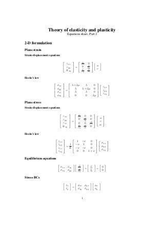
- 1. Theory of elasticity and plasticity Equations sheet, Part 2 2-D formulation Plane strain Strain-displacement equations εxx εyy 2εxy = ∂ ∂x 0 0 ∂ ∂y ∂ ∂y ∂ ∂x u v Hooke’s law σxx σyy σzz σxy = λ + 2µ λ 0 λ λ + 2µ 0 λ λ 0 0 0 2µ εxx εyy εxy Plane stress Strain-displacement equations εxx εyy εzz 2εxy = ∂ ∂x 0 0 0 ∂ ∂y 0 0 0 ∂ ∂z ∂ ∂y ∂ ∂x 0 u v w Hooke’s law εxx εyy εzz εxy = 1 E 1 −ν 0 −ν 1 0 −ν −ν 0 0 0 1 + ν σxx σyy σxy Equilibrium equations σxx σxy σxy σyy ∂ ∂x ∂ ∂y + fx fy = 0 0 Stress BCs tx ty = σxx σyx σxy σyy nx ny 1
- 2. Airy stress function σxx = ∂2 φ ∂y2 , σyy = ∂2 φ ∂x2 , σxy = − ∂2 φ ∂x∂y where φ = φ(x, y) is an arbitrary form called an Airy stress function Biharmonic equation ∂4 φ ∂x4 + 2 ∂4 φ ∂x2∂y2 + ∂4 φ ∂y4 = 0 Polynomial solution of 2-D problem Main steps • Select the polynomial function φ(x, y) = C1x2 + C2xy + C3y2 + C4x3 + . . . • Check the compatibility condition (biharmonic equation) 2 2 φ(x, y) = 0 • Use the Strong and Weak BCs to obtain a set of equations for Ci • Solve all equations and determine Ci FEM in plane elasticity- Constant Strain Triangle Displacement interpolation ux uy = ζ1 0 ζ2 0 ζ3 0 0 ζ1 0 ζ2 0 ζ3 ux1 uy1 ux2 uy2 ux3 uy3 Strain-displacement matrix B = 1 2A y23 0 y31 0 y12 0 0 x32 0 x13 0 x21 x32 y23 x13 y31 x21 y12 where 2A = det 1 1 1 x1 x2 x3 y1 y2 y3 and xjk = xj − xk, yjk = yj − yk 2
- 3. Element stiffness matrix k = A hBT E BdA where E = E 1 − ν2 1 ν 0 ν 1 0 0 0 1−ν 2 Classical plate theory Displacement, curvature and strain fields u(x, y, z) v(x, y, z) w(x, y, z) = −z ∂w0 ∂x −z ∂w0 ∂y w0(x, y) , κxx κyy κxy = −∂w2 ∂x2 −∂w2 ∂y2 −2 ∂w2 ∂x∂y , εxx εyy εxy = z κxx κyy κxy Stresses, stress resultants σxx σyy σxy = E 1 − ν2 1 ν 0 ν 1 0 0 0 1−ν 2 z κxx κyy κxy , Mxx Myy Mxy = D 1 ν 0 ν 1 0 0 0 1−ν 2 κxx κyy κxy where the flexural rigidity is D = Et3 12(1−ν2) Equilibrium equation ∂4 w ∂x4 + 2 ∂4 w ∂x2∂y2 + ∂4 w ∂y4 = q D Boundary conditions (edge, orthogonal of the x-axis) • Fixed edge- w = 0, dw dx = 0 • Free edge- Mx = 0, Vx = 0, where Vx = Qx + ∂Mxy ∂y • Simply supported edge- Mx = 0, w = 0 Navier’s solution • Furier series coefficient of the loading qmn = 4 ab b 0 a 0 q(x, y) sin mπ a x sin nπ b ydxdy 3
- 4. • Solution for the displacement w(x, y) = 1 Dπ4 ∞ m=1 ∞ n=1 qmn m2 a2 + n2 b2 2 sin mπ a x sin nπ b y Marcus Method BCs cases Lx Ly Case 1 Lx Ly Case 2 Lx Ly Case 3 Lx Ly Case 4 Lx Ly Case 5 Lx Ly Case 6 Cx = 1 Cx = 2 Cx = 1 Cx = 1 Cx = 1 Cx = 1 Cy = 1 Cy = 5 Cx = 5 Cx = 1 Cx = 2 Cx = 1 Directional loads qx = Cy 4 y Cx 4 x + Cy 4 y q, qy = q − qx Bending moments • Maximum span moments Mx = ¯Mx 1 − 5 6 2 x 2 y ¯Mx M0 x , My = ¯My 1 − 5 6 2 y 2 x ¯My M0 y where ¯Mx and ¯My are maximum span moments in strips loaded by the corresponding directional load and M0 x = q 2 x 8 , M0 y = q 2 y 8 • Edge moments- the edge moments are calculated as a strip supported with the same type of supports as a plate and loaded with directional load qx or qy 4